摘要:复杂网络中节点重要性的评估是网络特性研究中的一项重要课题, 相关研究具有广泛的应用. 目前提出了许多方法来评估网络中节点的重要性, 然而大多数方法都存在评估角度片面或者时间复杂度过高的不足. 为了突破现有方法的局限性, 本文提出了一种基于Tsallis熵的复杂网络节点重要性评估方法. 该方法兼顾节点的局部和全局拓扑信息, 综合考察节点的结构洞特征和K壳中心性, 并充分考虑节点及其邻域节点的影响. 为了验证该方法的有效性, 本文采用单调性指标、SIR模型和Kendall相关系数作为评价标准, 在8个来自不同领域的真实网络上与其他方法进行比较. 实验结果表明, 此方法能更有效和准确地评估网络节点的重要性, 可以显著区分不同节点的重要性. 此外, 该方法的时间复杂度仅为$ O({n^2}) $, 适用于大型复杂网络.
关键词: 节点重要性/
Tsallis熵/
结构洞/
K壳

English Abstract

全文HTML

--> --> -->

随着网络信息技术的发展与进步, 对复杂网络的研究已经在许多领域受到关注. 关键节点作为复杂网络的核心要素之一, 对网络的结构和功能有着重要影响, 被广泛的研究与应用^[1-3]. 例如, 通过对电力网络中某关键的调度中心和变电所进行维保, 能保证整个电力网络正常运转的稳定性与高效性^[4]; 通过对病毒传播网络中超级传播源实施隔离, 能够大幅降低病毒的传播速度和减小扩散范围^[5]; 通过对社交网络中核心的言论加以控制, 能够有效促进或抑制信息的传播^[6]. 因此, 评估网络中节点重要性具有重大意义.
在不同研究背景下, 研究人员提出了众多节点重要性评估方法. 目前, 度中心性^[7]是评估网络节点重要性的常用方法, 该方法简单但不够精准. 介数中心性^[8]和接近中心性^[9]分别考虑的是节点间的最短路径数量和平均最短距离, 此类方法从全局信息的角度出发, 效果明显但计算时间复杂度较高, 不适用于大型复杂网络. Kitsak等^[10]依据网络中节点处于网络的核心位置往往有较高影响力的思想, 提出用K壳分解法确定网络中节点的位置, 此方法时间复杂度低, 适用于大型复杂网络, 然而其区分度过于粗粒化. 为了提高节点区分度, Zeng等^[11]提出了混合度分解(mixed degree decomposition, MDD)法, 以网络中剩余的邻居节点以及删除的邻居节点的混合度进行K壳分解. Bae和Kim^[12]在改进K壳算法时提出了邻域核心的概念, 利用节点自身及其邻居的K壳值之和来评估网络中节点的重要性. Hou等^[13]考虑多指标评估, 基于欧拉距离公式计算节点的度值、介数、K壳等3个不同指标的组合度量, 更为综合地评估了节点的重要性. 王凯莉等^[14]提出了一种基于多阶邻居壳数的向量中心性方法, 利用向量的形式来表示节点在网络中的相对重要性. Burt等^[15]提出经典社会学中的“结构洞”理论, 设计了网格约束系数来量化节点形成结构洞时所受到的约束, 该方法利用了节点的局部信息, 具有良好的精度和较低的计算时间复杂度. 苏晓萍和宋玉蓉^[16]提出一种基于节点及其邻域结构洞的评估节点重要性的方法, 该方法综合考虑了节点及其邻域的度值和拓扑结构, 能有效评估网络中节点的重要性. 韩忠民等^[17]提出了一种融合结构洞等7个度量指标的方法, 该方法利用基于ListNet的排序学习方法, 能够较为全面地评估网络中节点的重要性.
当使用熵来评估复杂网络时, 复杂网络的结构越有序, 熵值就越小, 反之亦然. 同时, 熵也可用来描述整个网络结构的复杂性和复杂网络的统计特性. 例如, Chen等^[18]提出了结构熵来量化复杂网络的结构特征. Zhang等^[19]提出了一种基于非广延统计力学的结构熵来度量网络的复杂性. 黄丽亚等^[20]提出了一种基于网络节点在K步内可达的节点总数的K-阶结构熵, 用于度量复杂网络的异构性. Wang等^[21]提出了一种基于K壳和节点信息熵的改进算法, 用于区分上层外壳和下层外壳中节点的重要性.
受到上述研究工作的启发, 本文提出了一种基于Tsallis熵的复杂网络节点重要性评估方法(TSM). 该方法不仅考虑了节点的结构洞特征和K壳中心性, 还充分考虑了节点自身及其邻域节点的影响, 在兼顾节点的局部和全局拓扑信息的同时, 采用Tsallis熵来度量网络结构的复杂性. 时间复杂度分析表明, 该方法的时间复杂度仅为$ O({n^2}) $, 适用于大型复杂网络. 为了说明该方法的有效性和适用性, 本文选用了8个来自不同领域的真实网络, 并采用了7个现有的节点重要性评估方法作为比较方法. 在此基础上, 利用单调性指标、SIR模型和Kendall相关系数$ \tau $说明了该方法的优越性以及不同方法之间的关系.

2

-->

2.1.网络定义

设图$ G = (V, E) $是1个无向无权网络, 其中$V = \{ {v_1}, {v_2}, \cdots, {v_n}\}$表示$ G $中节点的集合, $|V| = n$, $ E = \{ ({v_i}, {v_j})|{v_i}, {v_j} \in V\} $表示$ G $中边的集合, $|E| = $$ m$. 记$ {A_{n \times n}} = {({a_{ij}})_{n \times n}} $为$ G $对应的邻接矩阵, 如果节点$ {v_i} $和节点$ {v_j} $之间存在连边关系, 则$ {a_{ij}} = 1 $, 否则$ {a_{ij}} = 0 $.
2 -->

2.2.度中心性

度中心性(degree centrality, DC)^[7]是衡量节点影响力的最简单指标. 节点拥有的度数越大, 该节点的影响力就越大. 节点$ {v_i} $的DC定义为

$ {\rm{DC}}(i) = \sum\limits_{j = 1}^n {{a_{ij}}} , $

其中, $ n $为网络中节点的数量. 于是, 节点$ {v_i} $的邻接度可以定义为$Q(i) = \displaystyle\sum\nolimits_{\omega \in \varGamma (i)} {{\rm{DC}}(\omega )}$, 其中, $ \varGamma (i) $为节点$ {v_i} $的邻居节点的集合.
2 -->

2.3.介数中心性

介数中心性(betweenness centrality, BC)^[8]是基于节点的最短路径数定义的全局指标. 通常, 节点的BC越大, 该节点的影响力就越大. 节点$ {v_i} $的介数中心性定义为

$ {\rm{BC}}(i) = \sum\limits_{s \ne i \ne t} {\frac{{\sigma _{st}^i}}{{{\sigma _{st}}}}} , $

其中, $ {\sigma _{st}} $为网络中任意两个节点$ {v_s} $和$ {v_t} $之间的最短路径数目, $ \sigma _{st}^i $为经过节点$ {v_i} $的最短路径数目.
2 -->

2.4.混合度分解方法

混合度分解方法(mixed degree decomposition method, MDD)由Zeng等^[11]提出, 该方法有效提高了K壳分解方法的区分度. 它通过同时考虑节点的剩余度值$k_i^{\rm r}$和节点的已移除度值$k_i^{\rm e}$对K壳分解过程进行了改进, 网络按照新的混合度值继续分层, 节点$ {v_i} $的混合度定义为

$ k_i^{\rm m} = k_i^{\rm r}+ \lambda k_i^{\rm e}, $

其中, $ \lambda $是0到1之间的可调参数. 当$\lambda = 0$时, MDD方法与K壳分解方法一致, 但当$ \lambda = 1 $时, 它等同于DC. 在本文中, 设定了参考文献[11]中使用的参数$ \lambda = 0.7 $.
2 -->

2.5.全方位距离

Hou等^[13]提出了全方位距离(all-around distance, AAD)指标, 其综合考虑了节点的度值、BC、K壳等3个不同指标的影响, 采用欧拉距离公式计算了这3个指标的组合度量, 计算公式如下所示:

$ D(i) = \sqrt {{\rm{D}}{{\rm{C}}^2}(i) + {\rm{B}}{{\rm{C}}^2}(i) + {\rm{K}}{{\rm{S}}^2}(i)} \text{, } $

其中, ${\rm{ KS}}(i)$为节点$ {v_i} $的K壳值.
2 -->

2.6.改进的K壳方法

改进的K壳方法(improved K-shell method, IKS)由Wang等^[21]提出, 该方法结合了K壳分解方法和节点信息熵. 它按照K壳分层从大到小的顺序进行迭代, 在每层未被选中节点中选择节点信息熵最高的节点, 直至网络中所有节点都被选中为止, 节点$ {v_i} $的节点信息熵定义为

$ {e_i} = - \sum\limits_{j \in \varGamma (i)} {{I_j}\ln {I_j}} \text{, } $

其中, $\varGamma (i)$为节点$ {v_i} $的邻居节点的集合, ${I_i} = $$ {\rm{DC}}(i)\Big/\displaystyle\sum\nolimits_{j = 1}^n {{\rm{DC}}(j)}$.
2 -->

2.7.结构洞理论

结构洞理论(structural holes theory)是Burt等^[15]在1992年研究社交网络中的竞争关系时提出的. 在社会网络中, 结构洞是指个体之间为非冗余关系, 且存在互补信息的差距. 为了量化结构洞节点对这些关系的控制, Burt采用约束系数来测量结构洞中节点形成的约束. 当系数越小, 节点越容易形成结构洞, 节点的影响力越大. 节点$ {v_i} $的约束系数为

$ {\rm RC}_i = {\sum\limits_j {\left(L_{ij} + \sum\limits_{q( \ne i,j)} {L_{iq}} L_{qj}\right)} ^2} \text{, } $

其中, 节点$ {v_q} $是节点$ {v_i} $和节点$ {v_j} $的共同邻居节点; $ {L_{ij}} $表示在节点$ {v_i} $的所有邻居节点中节点$ {v_j} $所占的权重比例.
在计算节点的约束系数时, 考虑到节点及其邻域的度值和拓扑结构对节点重要性的影响将$ {L_{ij}} $定义为

$ {L_{ij}} = {{Q(j)}}\bigg/{{\displaystyle\sum\limits_{\upsilon \in \varGamma (i)} {Q(\upsilon )} }} . $

2 -->

2.8.Tsallis非广延统计力学

对于1个有限的离散概率集, Boltzmann-Gibbs熵^[22]被定义为

$ {S_{{\text{BG}}}} = - k\sum\limits_{i = 1}^N {{p_i}\ln {p_i}} , $

其中, $ k $是玻尔兹曼常数, $ {p_i} $满足标准化条件$\displaystyle \sum\nolimits_{i = 1}^N {{p_i}} = 1 $.
1988年, 基于Boltzmann-Gibbs熵^[22]和Shannon熵^[23], Tsallis^[24]提出了一种新的熵, 它是一种更一般的形式, 能够描述广延的和非广延的系统, 被定义为

$ {S_q} = k\sum\limits_{i = 1}^N {{p_i}} {\ln _q}\frac{1}{{{p_i}}} . $

(9)式中的$ q $-对数函数为

$ {\ln _q}{p_i} = \frac{{p_i^{1 - q} - 1}}{{1 - q}}({p_i} > 0;q \in R;{\ln _1}{p_i} = \ln {p_i}) \text{, } $

$ \begin{split}&{\ln _q}\frac{1}{{{p_i}}} = \frac{{{{\dfrac{1}{{{p_i}}}}^{1 - q}} - 1}}{{1 - q}}=\frac{{p_i^{q - 1} - 1}}{{1 - q}}\\&({p_i} > ~ 0;q \in R; ~{\ln _1}{p_i} = \ln {p_i}), \end{split} $

根据(11)式可以将(9)式改写为

$ {S_q} = k\sum\limits_{i = 1}^N {{p_i}\frac{{ p_i^{q - 1} - 1}}{{1 - q}}} \text{, } $

$ {S_q} = k\sum\limits_{i = 1}^N {\frac{{ p_i^q - {p_i}}}{{1 - q}}} . $

由于$ {p_i} $满足标准化条件 $\displaystyle \sum\nolimits_{i = 1}^N {{p_i}} = 1$, (13)式可以进一步简化为

$ {S_q} = k\frac{{1 - \displaystyle \sum\limits_{i = 1}^N { p_i^q} }}{{q - 1}} \text{, } $

其中, N是子系统的数量. 将非广延参数$ q $用于描述子系统之间相互作用, 当$ q = 1 $时, Tsallis熵将退化为Boltzmann-Gibbs熵.

2

-->

3.1.方法构造

基于Tsallis熵的节点重要性评估方法构造的基本思想是在综合考虑节点的结构洞特征和K壳中心性的同时, 利用Tsallis熵度量网络结构的复杂性, 评估网络中节点的重要性. 由于结构洞特征能体现节点的局部拓扑信息, 而K壳中心性表征了节点的全局拓扑信息, 结合这两种拓扑信息, 利用Tsallis熵度量网络结构复杂性, 并通过对每个节点的自身及其邻域节点的综合考察, 可以给出1个合理的评估网络中节点重要性的方法, 即本文提出的TSM方法.
基于Tsallis非广延统计力学, 可以得到Tsallis熵的如下形式:

$ T({v_i}) = \frac{{1 - \displaystyle \sum\nolimits_{j = 1}^n {{P_{ij}}^{{q_i}}} }}{{{q_i} - 1}} . $

因为结构洞约束系数是基于网络局部拓扑信息的评估指标, 考虑到相邻节点的结构洞特征对该节点重要性的影响, 可以得到$ {P_{ij}} $的定义:

$ {P_{ij}} = \frac{{1 - {\rm{R}}{{\rm{C}}_j}}}{{\displaystyle \sum\limits_{j \in \varGamma (i)} {(1 - {\rm{R}}{{\rm{C}}_j})} }} . $

由于K壳中心性是描述节点在网络中所处位置的全局指标, 因此它可以用来表示每个节点与整个网络之间的关系以及不同节点之间的关系. 本文运用MDD方法得到节点$ {v_i} $的K壳中心性${\rm Ks}_i$及其与网络中所有节点的K壳中心性数值之和的比值. 进而, 可得到节点$ {v_i} $的Tsallis参数$ {q_i} $:

$ {q_i} = 1 + \frac{{{\rm Ks}_i }}{{\displaystyle \sum\nolimits_{j = 1}^n {{\rm Ks}_j} }} . $

(17)式的目的是使参数$ {q_i} $＞1, 以反映子系统对网络的次可加性影响. 在信息论中, 不同的$ q $值表示不同子系统对Tsallis熵的可加性不同, 即$ q < 1 $, $ q = 1 $, $ q > 1 $分别代表超可加性、可加性和次可加性. 扩展到复杂网络中, 整个网络可以看作1个系统, 每个节点和相应的连边可以看作网络的子系统.
利用Tsallis熵度量网络结构复杂性得到$ T({v_i}) $后, 再结合节点自身的结构洞特征, 可得

$ {\rm{IC}}({v_i}) = (1 - {\rm{R}}{{\rm{C}}_i}) \cdot T({v_i}). $

Bae和Kim^[12]在改进K壳算法时提出了邻域核心的概念, 通过对所有邻居的K壳值进行求和来衡量网络中节点的重要性. 本文借鉴了这一概念, 充分考虑邻域节点的影响. 对于节点$ {v_i} $, 将其所有相邻节点的IC值进行相加, 得到节点$ {v_i} $的邻域核心(核心邻域中心性) Cnc(v_i):

$ {\rm{Cnc}}({v_i}) = \sum\limits_{j \in \varGamma (i)} {{\rm{IC}}({v_i})} . $

在(19)式的基础上, 对其所有相邻节点的邻域核心值Cnc进行求和, 可以得到节点$v_i$的扩展邻域核心Cnc₊(v_i), 最终得到了节点$v_i$的重要性评估值TSM(v_i):

$ {\rm{TSM}}({v_i}) = {\rm{Cn}}{{\rm{c}}_ + }({v_i}) = \sum\limits_{j \in \varGamma (i)} {{\rm{Cnc}}({v_i})} . $

2 -->

3.2.时间复杂度分析

本节将对本文提出的TSM算法进行计算时间复杂度分析, 其具体计算步骤如表1所列. 由表1可知, TSM要遍历网络中每个节点, 在计算节点的结构洞约束系数值RC_i时, 考虑了节点的度及其与邻居拓扑结构间的关系, 故时间复杂度应为$ O({n^2}) $; 在计算Tsallis参数$ {q_i} $时, 采用了MDD方法得到节点的K壳重要性指标, 其时间复杂度为$ O(n) $; 在计算节点的$ T_i $值时, 需要考虑节点的邻居节点信息, 则时间复杂度为$ O(n * k) $; 而在对IC进行累加时, 时间复杂度为$ O(n) $. 由此可以看出, TSM算法的时间复杂度取决于节点的结构洞约束系数值RC_i的计算, 因此本文提出的TSM算法的时间复杂度为$ O({n^2}) $. 其中, $ n $为网络中节点的总数, $ k $为网络的平均度.

Algorithm 1: TSM algorithm.

Input: Network $ G(V, E) $ Output: TSM value for each node 1. Find neighboring nodes $\varGamma (i)$of node $ {v_i} $ 2. Compute the restraint coefficient ${\rm{RC}}_i$ of node $ {v_i} $ 3. Compute the ${\rm Ks}_i$ value of node $ {v_i} $according to formula $k_i^{\rm m} = k_i^{\rm r} + \lambda k_i^{\rm e}$ 4. Compute $ {q_i} $ for node $ {v_i} $ 5. For node $ {v_j} $ in $\varGamma (i)$ do 6. ratio = ($1 - {\rm{RC}}_j$)/${\rm{sum}}$($1 - {\rm{RC}}$(all neighbors of $ {v_i} $)) 7. $ T({v_i}) $= (pow(ratio, $ {q_i} $)-ratio)/(1 – $ {q_i} $) 8. End For 9. Compute ${\rm{IC} }\left( { {v_i} } \right) = \left( {1 - {\rm{RC} }_i } \right)*T\left( { {v_i} } \right)$ 10. For node $ {v_j} $ in $\varGamma (i)$ do 11. ${\rm{Cnc}}\left( { {v_i} } \right) = {\rm{sum}}\left( {{\rm{IC}}\left( { {v_j} } \right)} \right)$ 12. End For 13. For node $ {v_j} $ in $\varGamma (i)$ do 14. ${\rm{TSM}}\left( { {v_i} } \right) = {\rm{sum}}\left( {{\rm{Cnc}}\left( { {v_j} } \right)} \right)$ 15. End For

表1计算步骤
Table1.Step of the calculation.

表2列出了几种不同方法的时间复杂度, 并按照评估方法所包含的网络信息将这些方法分成了局部、全局、混合等3个类型. 其中, $ m $为网络中连边的总数. 当$ n < m $时, 有$ O(n) < O({n^2}) < O(nm) $, $ O({n^2}) < O({n^3}) $. 可以看出, TSM的时间复杂度并不是最低, 但其精度显著优于其他方法(见表5和图3), 且节点包含的网络信息要远高于其他方法. 因此, TSM方法适用于大型网络.

Method	Category	Time complexity
$ {\text{DC}} $	Local	$ O(n) $
$ {\text{BC}} $	Global	$ O({n^3}) $or$ O(nm) $
$ {\text{MDD}} $	Global	$ O(n) $
${\text{N-Burt} }$	Local	$ O({n^2}) $
$ {\text{Cnc + }} $	Hybrid	$ O(n) $
$ {\text{AAD}} $	Hybrid	$ O({n^3}) $ or $ O(nm) $
$ {\text{IKS}} $	Hybrid	$ O(n) $
$ {\text{TSM}} $	Hybrid	$ O({n^2}) $

表2不同方法的时间复杂度
Table2.Time complexity of different methods.

2

-->

4.1.实验数据

本文选用了8个来自不同领域的真实网络进行实验, 分别是: 空手道俱乐部社交网络Karate network^[25]、海豚社交网络Dolphins network^[26]、美国政治书籍网络Polbooks network^[27]、爵士音乐家网络Jazzmusic network^[28]、美国航空运输网络USAirline network^[29]、秀丽隐杆线虫网络C.Elegans network^[30]、大学电子邮件网络Email network^[31]、美国电力网络PowerGrid network^[1]. 各网络的统计特征如表3所列. 其中$ n $为节点总数, $ m $为连边总数, $ \langle k \rangle $为平均度, $ c $为聚类系数, $ \langle d \rangle $为平均最短路径长度, ${\beta _{{\text{th}}}}$为SIR模型传播率阈值, $\beta $为实际传播率取值.

Network	$ n $	$ m $	$\langle k \rangle$	$ c $	$\langle d \rangle$	${\beta _{\rm th} }$	$\beta $
Karate	34	78	4.5880	0.5706	2.4082	0.1287	0.25
Dolphins	62	159	5.1290	0.2590	3.3570	0.1470	0.15
Polbooks	105	441	8.4000	0.4880	3.0788	0.0838	0.10
Jazz	198	2742	27.6970	0.6175	2.2350	0.0259	0.04
USAir	332	2126	12.8072	0.7494	2.7381	0.0225	0.03
C.Elegans	453	2025	8.9404	0.6465	2.4553	0.0249	0.03
Email	1133	5451	9.6222	0.2540	3.6060	0.0535	0.05
PowerGrid	4941	6594	2.6691	0.0801	18.9892	0.2583	0.25

表3网络的统计特征
Table3.Statistical characteristics of the networks.

2 -->

4.2.有效性分析

为了验证本文提出的TSM算法的有效性和准确性, 首先以Karate网络为例进行仿真分析, 其拓扑图如图1所示. 选用了DC^[7]、 BC^[8]、 MDD^[11]、邻域结构洞方法^[16] (N-Burt)、核心邻域中心性^[12] (Cnc₊)、AAD ^[13]以及IKS^[21]等7种方法与本文提出的TSM方法进行对比, 得到网络前15个关键节点的重要性评估结果如表4所列.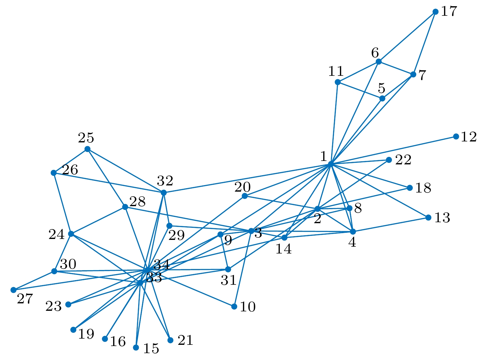
图 1 Karate网络的拓扑结构
Figure1. Topological structure of the Karate network.

排名	节点	DC	节点	BC	节点	MDD	节点	N-Burt	节点	Cnc+		节点		AAD	节点	IKS	节点	TSM
1	${v_{34}}$	17	${v_1}$	0.4119	${v_{34}}$	11.9	${v_{34}}$	0.1682	${v_{34}}$	1156		${v_{34}}$		17.4666	${v_1}$	1.5215	${v_{34}}$	89.8687
2	${v_1}$	16	${v_{34}}$	0.2862	${v_1}$	11.2	${v_1}$	0.1731	${v_1}$	1024		${v_1}$		16.4976	${v_{34}}$	1.4782	${v_1}$	81.8535
3	${v_{33}}$	12	${v_{33}}$	0.1367	${v_{33}}$	8.7	${v_3}$	0.2257	${v_{33}}$	576		${v_{33}}$		12.6498	${v_3}$	1.2610	${v_{33}}$	72.0759
4	${v_3}$	10	${v_3}$	0.1352	${v_3}$	7.6	${v_{33}}$	0.2746	${v_3}$	400		${v_3}$		10.7712	${v_{33}}$	1.2307	${v_3}$	70.7235
5	${v_2}$	9	${v_{32}}$	0.1301	${v_2}$	6.9	${v_{32}}$	0.2793	${v_2}$	324		${v_2}$		9.8490	${v_2}$	1.0208	${v_2}$	59.4435
6	${v_4}$	6	${v_9}$	0.0526	${v_4}$	5.1	${v_9}$	0.3266	${v_4}$	144		${v_4}$		7.2111	${v_9}$	0.9425	${v_9}$	47.6431
7	${v_{32}}$	6	${v_2}$	0.0508	${v_{32}}$	5.1	${v_2}$	0.3357	${v_{32}}$	108		${v_{32}}$		6.7095	${v_{14}}$	0.9411	${v_{14}}$	46.9374
8	${v_9}$	5	${v_{14}}$	0.0432	${v_{14}}$	5	${v_{14}}$	0.3541	${v_9}$	100		${v_9}$		6.4033	${v_{32}}$	0.9004	${v_4}$	45.5295
9	${v_{14}}$	5	${v_{20}}$	0.0306	${v_9}$	4.7	${v_{28}}$	0.3674	${v_{14}}$	100		${v_{14}}$		6.4033	${v_4}$	0.8343	${v_{32}}$	41.3938
10	${v_{24}}$	5	${v_6}$	0.0282	${v_{24}}$	4.1	${v_{31}}$	0.3810	${v_{24}}$	75		${v_{24}}$		5.8310	${v_{31}}$	0.7137	${v_{31}}$	37.1209
11	${v_6}$	4	${v_7}$	0.0282	${v_8}$	4	${v_{20}}$	0.3935	${v_8}$	64		${v_{31}}$		5.6569	${v_{24}}$	0.7027	${v_8}$	35.7453
12	${v_7}$	4	${v_{28}}$	0.0210	${v_{31}}$	4	${v_{29}}$	0.4115	${v_{31}}$	64		${v_8}$		5.6569	${v_8}$	0.6996	${v_{24}}$	33.3428
13	${v_8}$	4	${v_{24}}$	0.0166	${v_{28}}$	3.7	${v_{24}}$	0.4348	${v_6}$	48		${v_6}$		5.0001	${v_{20}}$	0.6397	${v_{28}}$	29.9028
14	${v_{28}}$	4	${v_{31}}$	0.0136	${v_{30}}$	3.7	${v_4}$	0.4684	${v_7}$	48		${v_7}$		5.0001	${v_{30}}$	0.6050	${v_{20}}$	29.6927
15	${v_{30}}$	4	${v_4}$	0.0112	${v_6}$	3.4	${v_{26}}$	0.4845	${v_{28}}$	48		${v_{28}}$		5.0000	${v_{28}}$	0.6039	${v_{30}}$	29.1552

表4Karate网络的节点重要度评估结果
Table4.Node importance evaluation results in the Karate network.

通过结合Karate网络拓扑结构(图1)与重要性评估结果(表4)分析可知: 节点$ {v_4} $和节点$ {v_{32}} $拥有的邻居数量均为6且其所处的网络信息传输位置相同, 而在其他方法中节点$ {v_4} $和节点$ {v_{32}} $的重要性是不一样的; 节点$ {v_9} $, $ {v_{14}} $, $ {v_{24}} $拥有的邻居数量相同均为5, 而它们存在的邻域结构洞差值较大, 因此, 仅仅考虑节点拥有的邻居数量和其所处的网络信息传输位置无法进一步区分节点的重要性. 采用N-Burt方法评估节点重要性时, 未考虑到相邻节点的结构洞特征对节点重要性的影响, 如节点$ {v_{32}} $比节点$ {v_4} $存在更多的结构洞, 但节点$ {v_4} $的相邻节点较节点$ {v_{32}} $的相邻节点在网络中是更为重要的“桥接”节点, 信息能通过它们更快地扩散至网络. BC是一种能够很好地体现节点在网络信息传播过程中的重要性的方法, 但是对于一些不在任何一条最短路径上的节点以及信息负载能力相似的节点, 如节点$ {v_6} $, $ {v_7} $, $ {v_8} $, $ {v_{28}} $等仍需要进一步考虑节点的局部信息来评估, 而且此方法的计算时间复杂度较高.
本文所提出的TSM方法克服了以上方法的不足, 它从节点的局部和全局拓扑信息两个角度出发, 综合考虑节点自身的结构洞特征和网络位置信息以及邻域节点的影响, 并基于Tsallis熵度量网络结构的复杂性, 可提高节点重要性的区分度, 准确地评估节点重要性. 如表4所列, 通过TSM方法评估出的前15个重要节点与其他方法评估出的重要节点基本相同, 说明TSM方法能够有效地评估节点的重要性. 在TSM方法中, 节点$ {v_4} $比节点$ {v_{32}} $更为重要, 这很好地体现了相邻节点的结构洞特征对节点的影响, 同时也说明本方法克服了BC的不足; 节点$ {v_9} $, $ {v_{14}} $, $ {v_{24}} $和节点$ {v_8} $, $ {v_{28}} $, $ {v_{30}} $的重要性得到了进一步的区分, 其中, 节点$ {v_9} $的重要性高于节点$ {v_{14}} $, 这说明了本方法既有效地识别了网络中的“桥接”节点, 亦克服了DC的不足. 通过对比, 本文提出的TSM方法能有效地评估节点重要性, 可进一步提高节点重要性的区分度.
2 -->

4.3.评价标准

接下来介绍验证所提出的TSM方法准确性的评价标准. 它们分别是单调性指标^[12]、SIR模型^[32]和Kendall相关系数^[33].
本文采用单调性指标^[12]$ M(R) $来量化不同重要性评估方法的分辨率, 如下所示:

$ M(R) = {\left[1 - \frac1{n(n - 1)} {{\displaystyle\sum\limits_{r \in R} {nr} (nr - 1)}} \right]^2} , $

其中, $ R $为评估方法得到的每个节点的重要性排序向量, $ n $为网络中节点的个数, $ nr $为重要性相同的节点的数量. $ M(R) $的取值介于0到1之间. 如果$ M(R) = 1 $, 则排序向量$ R $是完全单调的, 说明该评估方法能将网络中所有节点的重要性完全区分; 如果$ M(R) = 0 $, 则表示网络中所有节点的重要性相同.
目前, 大多数****采用标准的SIR模型^[32]来检测信息和病毒的传播能力. 在SIR模型中, 网络中的每个节点可以处于以下3种状态中的1种: 易感状态S (susceptible)、感染状态I (infected)以及恢复状态R (removed). 在传播初始阶段, 网络中只有节点$ {v_i} $处于感染状态, 其余节点均处于易感状态. 在每个时间步中, 处于状态I的节点以传播率$ \beta $尝试感染处于S状态的邻居节点, 同时以概率$ \mu $恢复成状态R后, 不再被感染. 传播过程结束的标志是网络中不再出现I态节点. 在整个SIR传播过程结束时, 将网络中处于状态R的节点的数量$ S(i) $看作节点$ {v_i} $的传播能力. 为不失一般性, 本文设定恢复率$ \mu = 1 $. 在设定传播率时, 如果传播率$ \beta $过小或过大, 都会导致传播过程无法正常进行, 从而无法准确衡量每个节点的传播能力. 因此, 本文设定传播率阈值为${\beta _{{\text{th}}}} \approx \langle k \rangle / \langle {k^2} \rangle$. 其中$\langle k \rangle$为网络平均度, $\langle {k^2} \rangle$为网络二阶邻居平均度. 为保证传播过程正常进行, 本文的传播率$ \beta $在传播率阈值$ {\beta _{{\text{th}}}} $附近取值.
为了评估节点重要性评估方法的精准度, 本文使用Kendall相关系数^[33]$ \tau $来度量每个评估方法得到的节点重要性排序列表R与从SIR模型获得的节点传播能力排序列表$\sigma $之间的相关性. 假设存在两个包含$n$个节点的序列$X$和$Y$, 其中$X = $$ \left( {{x_1}, {x_2}, \cdot \cdot \cdot , {x_n}} \right)$和$Y = \left( {{y_1}, {y_2}, \cdot \cdot \cdot , {y_n}} \right)$, 将序列$X$和序列$Y$中的元素一一对应构造1个新的序列$XY = \left( {\left( {{x_1}, {y_1}} \right), \cdot \cdot \cdot , \left( {{x_i}, {y_i}} \right), \cdot \cdot \cdot , \left( {{x_n}, {y_n}} \right)} \right)$. 而对于序列$XY$中的任意一对元素$X{Y_i} = \left( {{x_{i, }}{y_i}} \right)$和$X{Y_j} = $$ \left( {{x_j}, {y_j}} \right)$, 若${x_i} > {x_j}$且${x_i} > {y_j}$, 或${x_i} < {x_j}$且${x_i} < {y_j}$, 则认为这一对元素是同序的; 若${x_i} > {x_j}$且${x_i} < {y_j}$, 或${x_i} < {x_j}$且${x_i} > {y_j}$, 则认为这一对元素是异序的; 若${x_i} = {x_j}$且${x_i} = {y_j}$, 则认为这一对元素既不是同序的, 也不是异序的. 肯德尔相关系数$ \tau $计算公式为

$ \tau (X,Y) = \frac{{C - D}}{{n(n - 1)/2}} \text{, } $

其中, C和D分别表示同序对和异序对的数量. $ \tau $的取值介于–1和1之间, $ \tau = 1 $时表示两个序列完全正相关, 即相关系数$ \tau $越接近1, 精确度越高; 反之, 则表示完全负相关.
2 -->

4.4.实验分析

本节记录并分析了不同节点重要性评估方法在不同真实网络中的实验结果.

Network	$ M{\text{(DC)}} $	M (BC)	M (MDD)	$M{\text{(N-Burt)} }$	$ M{\text{(Cnc + )}} $	M (ADD)	$ M{\text{(IKS)}} $	$ M{\text{(TSM)}} $
Karate	0.7079	0.7723	0.7536	0.9542	0.9472	0.8395	0.9612	0.9542
Dolphins	0.8312	0.9623	0.9041	0.9623	0.9895	0.9623	0.9905	0.9979
Polbooks	0.8252	0.9974	0.9077	1	0.9971	0.9996	1	1
Jazz	0.9659	0.9885	0.9883	0.9983	0.9993	0.9981	0.9994	0.9994
USAir	0.8586	0.6970	0.8871	0.9453	0.9945	0.9068	0.9943	0.9951
C.Elegans	0.7922	0.8740	0.8748	0.9983	0.9980	0.9381	0.9974	0.9990
Email	0.8874	0.9400	0.9229	0.9650	0.9991	0.9629	0.9995	0.9999
PowerGrid	0.5927	0.8313	0.6928	0.8770	0.9568	0.8748	0.9667	0.9999

表5不同评估方法的单调性指标M
Table5.Monotonicity index M of different evaluation methods.

图 3 不同传播率下SIR和各评估方法之间的Kendall相关系数, 图中黑色虚线为传播阈值$ {\beta _{{\text{th}}}} $　(a) Karate网络; (b) Dolphins网络; (c) Polbooks网络; (d) Jazz网络; (e) USAir网络; (f) C.Elegans网络; (g) Email网络; (h) PowerGrid网络
Figure3. Kendall correlation coefficient between SIR and the evaluation methods under different transmission rates, the black dashed line in the figure is the propagation threshold $ {\beta _{{\text{th}}}} $: (a) Karate network; (b) Dolphins network; (c) Polbooks network; (d) Jazz network; (e) USAir network; (f) C.Elegans network; (g) Email network; (h) PowerGrid network.

首先选用了DC, BC, MDD, N-Burt, Cnc+, AAD以及IKS等7种评估方法作为对比方法, 利用单调性指标^[12]M考察了7种对比方法与本文所提出的TSM方法的分辨率, 即对节点重要性的区分度. 表5记录了不同评估方法在8个真实网络中的分辨率, 并在图2中更为直观地呈现了它们之间的差异. 从图2可以看出, TSM方法在8个真实网络中表现十分出色. 此外, Cnc+和IKS方法的区分度也很好. 与其他7种方法相比, TSM方法大多数情况下可以给出更高M值, 而且在所有网络中M (TSM)都非常接近甚至等于1. 因此, TSM方法能够更好地区分节点的重要性.
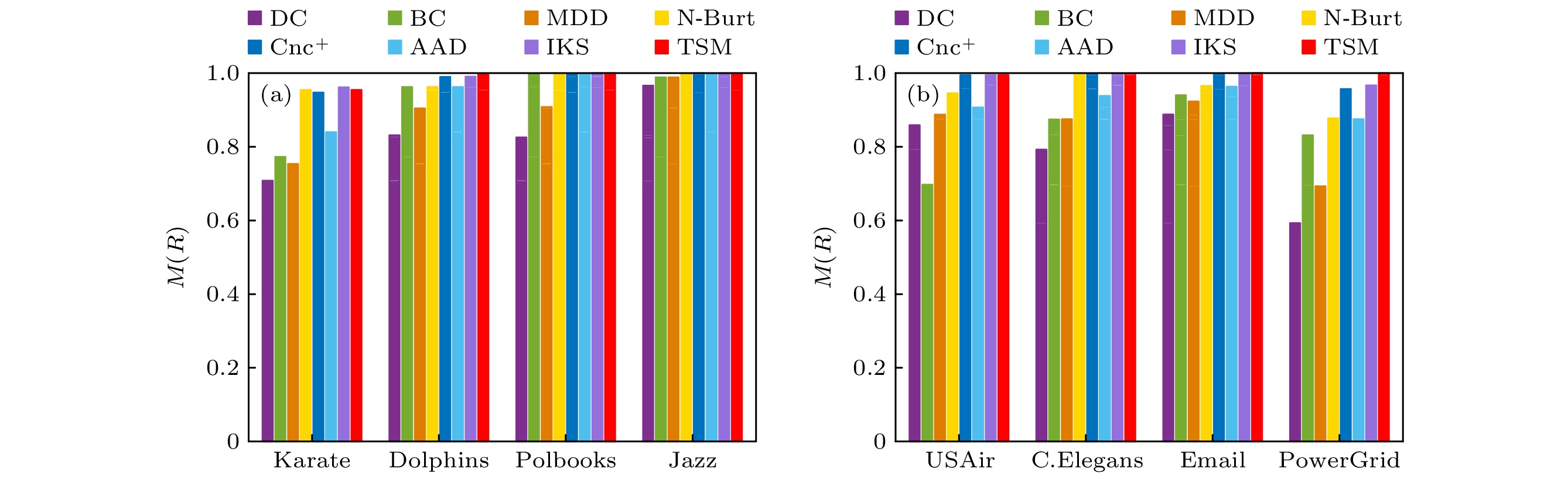图 2 不同评估方法的单调性指标M　(a) Karate网络、Dolphins网络、Polbooks网络和Jazz网络; (b) USAir网络、C.Elegans网络、Email网络和PowerGrid网络
Figure2. Monotonicity index M of different evaluation methods: (a) Karate network, Dolphins network, Polbooks network and Jazz network; (b) USAir network, C.Elegans network, Email network and PowerGrid network.

其次, 使用SIR模型得到节点的传播能力排序$\sigma $, 并计算了不同评估方法的排序与$\sigma $之间的Kendall相关系数$\tau $. 相关性越高, 对节点重要性的评估就越准确. 由于SIR模型迭代过程的随机性, 本文对每个节点重复模拟该过程, 然后取其平均值. 模拟将遵循以下规则: 对于网络|V | < 100, 模拟迭代10⁴次; 对于$ 100 < |V| < 10^4 $, 模拟迭代10³次. 表6展示了8个真实网络在选定传播率下各评估方法的Kendall相关系数, SIR模型的实际传播率取值如表3所列. 从表6可以看出, TSM方法的相关系数值在0.8到1之间. 同时, 与其他方法相比, TSM方法的相关性在8个真实网络中都最为显著. 因此, TSM方法的准确性得到了初步的验证.

Network	$\tau ({\text{DC, }}\sigma {\text{)}}$	$\tau ({\text{BC, }}\sigma {\text{)}}$	$\tau ({\text{MDD, }}\sigma {\text{)}}$	$\tau ({\text{N-Burt, } }\sigma {\text{)} }$	$\tau ({\text{Cnc + , }}\sigma {\text{)}}$	$\tau ({\text{AAD, }}\sigma {\text{)}}$	$\tau ({\text{IKS, }}\sigma {\text{)}}$	$\tau ({\text{TSM, }}\sigma {\text{)}}$
Karate	0.6435	0.5651	0.6756	0.7683	0.9258	0.6591	0.8445	0.9637
Dolphins	0.7768	0.5643	0.8181	0.7282	0.8611	0.7532	0.8526	0.9492
Polbooks	0.7528	0.3579	0.8029	0.7037	0.9098	0.7691	0.9165	0.9436
Jazz	0.8185	0.4628	0.8503	0.8216	0.9132	0.8235	0.8804	0.9363
USAir	0.6982	0.4744	0.7175	0.7929	0.9047	0.6995	0.9055	0.9461
C.Elegans	0.6376	0.4711	0.6521	0.6251	0.8127	0.659	0.8217	0.8570
Email	0.7911	0.6467	0.8015	0.7735	0.8980	0.7797	0.8758	0.9250
PowerGrid	0.5469	0.4167	0.5786	0.4298	0.7341	0.5563	0.7399	0.8207

表6选定传播率下SIR和各评估方法之间的Kendall相关系数
Table6.Kendall correlation coefficient between SIR and evaluation methods under a certain transmission rate.

为了进一步验证所提方法的准确性和可靠性, 对比了不同传播率下各评估方法与SIR模型排序结果之间的Kendall相关系数, 如图3所示. 从图3可以看出, 当传播率$ \beta $在传播阈值$ {\beta _{{\text{th}}}} $附近取值时, TSM方法的相关系数除了在Karate网络中略低于Cnc+方法以外, 在大多数情况下都高于其他方法, 与SIR模型得到的节点传播能力有显著的相关性. 同时, 可以看出当传播率$ \beta $远大于或者远小于传播阈值$ {\beta _{{\text{th}}}} $时, 在除Karate, USAir和PowerGrid网络以外的5个真实网络中, DC, MDD以及AAD等方法表现出了比TSM方法更好的相关性. 而BC的相关性在8个真实网络中表现最差. 因此, TSM方法能够更为准确地评估节点的重要性.
然后, 对Kendall相关系数的考察节点范围进行了调整, 将考察的节点从整体节点变为部分节点, 进一步研究了各个评估方法得到的不同比例排序靠前的节点与节点传播能力排序的相关性结果. 在8个真实网络中进行实验, 设置节点比例L的变化范围为0.05—1. 如图4所示, 给出不同比例节点下各评估方法的相关系数值. 从图4可以看出, 本文提出的TSM算法在不同比例节点下都能取得不错的节点重要性评估结果, 且在更大范围的L值下可以取得更好的评估结果.
图 4 不同比例节点下各评估方法的Kendall相关系数　(a) Karate网络; (b) Dolphins网络; (c) Polbooks网络; (d) Jazz网络; (e) USAir网络; (f) C.Elegans网络; (g) Email网络; (h) PowerGrid网络
Figure4. Kendall correlation coefficient of the evaluation methods under different proportion nodes: (a) Karate network; (b) Dolphins network; (c) Polbooks network; (d) Jazz network; (e) USAir network; (f) C.Elegans network; (g) Email network; (h) PowerGrid network.

最后, 分析了TSM方法与其他评估方法之间的关系, 如图5所示. 图中每个点代表复杂网络中的1个节点, 点的颜色表示由SIR模型得到的节点传播能力, 横轴和纵轴分别为TSM方法和其他方法得到的网络中各节点重要性数值. 当图中的节点呈线性分布时, 说明TSM方法与该方法有强的相关性. 从图5中的节点分布情况可以发现, TSM与DC, MDD, N-Burt之间存在强的相关性, 这说明TSM方法既充分考虑了节点的DC和位置信息, 而且有能力识别到网络中的“桥接”节点. 此外, TSM与Cnc+, AAD, IKS之间节点分布呈较明显的线性关系, 这说明节点重要性排名总体相似, 亦证明TSM方法能有效评估节点重要性. 从图5还可以发现, 有一些节点尽管其BC数值大, 但其传播能力并不是很强, 因此仅靠BC评估节点的重要性并不准确. 所以在评估网络中节点的重要性上, TSM方法较其他方法更有优势.
图 5 TSM与其他评估方法之间的关系　(a) Karate网络, β = 0.25; (b) Dolphins网络, β = 0.15; (c) Polbooks网络, β = 0.1; (d) Jazz网络, β = 0.04
Figure5. Relationship between TSM and other evaluation methods (a) Karate network, β = 0.25; (b) Dolphins network, β = 0.15; (c) Polbooksnetwork, β = 0.1; (d) Jazz network, β = 0.04.

本文提出了一种TSM方法, 有效地对复杂网络中节点重要性进行评估和排序. TSM方法兼顾局部拓扑信息和全局拓扑信息, 结合了节点的结构洞特征和K壳中心性, 利用Tsallis熵度量网络结构的复杂性, 弥补了现存方法评估角度片面的不足, 优化了可用资源的利用, 使信息得以有效传播. 该方法在考虑节点的邻域结构和位置信息的同时, 有能力识别到网络中的“桥接”节点, 从而对复杂网络中节点的重要性进行有效的评估. 在8个真实网络上的实验结果表明, 与其他评估方法如DC, BC, MDD, N-Burt, Cnc+, AAD和IKS相比, TSM方法能更好地区分节点重要性的差异, 在不同比例节点下都能准确地评估节点的重要性. 此外, TSM方法的时间复杂度仅为$ O({n^2}) $, 适用于大型复杂网络. 寻找一种结合网络结构和传播动力学的更有效的方法来评估网络中节点的重要性仍然是一个长期的挑战. 未来的工作将集中在如何应用所提出的TSM方法来评估多层网络中的节点重要性.