四连杆膝关节假肢的动力学建模与分析$^{\bf 1)}$

删除或更新信息，请邮件至freekaoyan#163.com(#换成@)

本站小编 Free考研考试/2022-01-01

吕阳^*, 方虹斌^?^,^**^,^??, 徐鉴^?^,^**^,^??, 马建敏^*, 王启宁^***, 张晓旭^,^?^,^**^,^??^,²⁾

^*复旦大学航空航天系,上海 200433

^?复旦大学智能机器人研究院,上海 200433

^**上海智能机器人工程技术研究中心,复旦大学,上海 200433

^??智能机器人教育部工程研究中心,复旦大学,上海 200433

^***北京大学工学院,北京 100871

DYNAMIC MODELING AND ANALYSIS OF THE LOWER LIMB PROSTHESIS WITH FOUR-BAR LINKAGE PROSTHETIC KNEE$^{\bf 1)}$

Lü Yang^*, Fang Hongbin^?^,^**^,^??, Xu Jian^?^,^**^,^??, Ma Jianmin^*, Wang Qining^***, Zhang Xiaoxu^,^?^,^**^,^??^,²⁾

^*Department of Aeronautics and Astronautics,Fudan University,Shanghai 200433,China

^?Institute of AI and Robotics,Fudan University,Shanghai 200433,China

^**Shanghai Engineering Research Center of AI & Robotics,Shanghai 200433,China

^??Engineering Research Center of AI & Robotics,Ministry of Education,Shanghai 200433,China

^***College of Engineering,Peking University,Beijing 100871,China

通讯作者: 2)张晓旭,副研究员,主要研究方向：非线性动力学. E-mail:zhangxiaoxu@fudan.edu.cn

收稿日期:2020-02-15接受日期:2020-04-29网络出版日期:2020-07-18

基金资助:

1)国家重点研发计划.2018YFB1307305

Received:2020-02-15Accepted:2020-04-29Online:2020-07-18
作者简介 About authors

摘要
相比于单轴式膝关节,四连杆膝关节具有更好的仿生特性和运动安全性,因而在下肢假肢研究中得到广泛关注. 本研究以一款四连杆膝关节被动假肢为研究对象,主要关注足-地交互作用力以及膝关节单边接触力等强非线性因素对下肢假肢步态的影响. 为此,采用 Kelvin-Voigt 模型和库伦模型描述足-地接触力和摩擦力,并采用 Kelvin-Voigt 模型描述膝关节单边接触力,从而基于第一类拉格朗日方程建立假肢动力学模型. 本研究以步态实验测得的髋关节运动数据为模型的驱动信号,针对假肢的步态特征进行了数值分析. 计算结果显示,当膝关节液压阻尼器的刚度较小时,强非线性作用力会使假肢产生显著的亚谐波响应,进而导致步态周期失谐. 进一步研究发现,提胯行为能够避免步态周期失谐,这也为残疾人行走时的提胯等代偿行为提供了一种新的力学解释. 为了评价假肢步态与健康人实测步态的一致性,本研究进一步定义了步态相关系数并分析了膝关节液压阻尼器刚度、阻尼参数对相关系数的影响. 结果表明,通过合理的刚度、阻尼参数设计,两者步态的相关系数可达到 0.9 以上,这为四连杆膝关节被动假肢进一步优化提供了理论支撑.
关键词： 非光滑接触力;步态实验;亚谐波响应;代偿行为;步态一致性

Abstract
The four-bar linkage prosthetic knee has attracted widespread attention in the study of lower limb prosthesis because it shows a better bionic feature and a higher locomotive safety than the uniaxial joint prosthetic knee. Based on a real four-bar linkage prosthetic knee, this paper mainly studies the strongly nonlinear effects, e.g. the foot-ground interaction force and the unilateral constraint force of knee joint, on the gait of the lower limb prosthesis. For this purpose, firstly, the Kelvin-Voigt contact model is adopted to represent the effect of foot-ground contact force and the unilateral constraint force of the knee joint. The Coulomb model is employed to describe the effect of foot-ground friction force. Then, the Lagrange equations of the first kind are applied to model the dynamics of the prosthesis. Based on this model, the measured hip joint motion of an able-bodied testee is used as the driven signal and the gait characteristics analysis is conducted numerically. The numerical results reveal that if the stiffness of the hydraulic cylinder, which supports the motion of the prosthetic knee joint, is small, the strongly nonlinear effects may lead to the remarkable subharmonic response, which further results in the so-called gait inconformity. Further research shows that the subharmonic response can be avoided by lifting the hip joint, which provides a new insight into the compensatory mechanism such as lifting the hip for the amputee walking from the view of mechanics. In order to evaluate the consistence of the gaits between the prosthesis and the able-bodied testee, this paper further defines the correlation coefficient and analyzes the effects of the hydraulic cylinder's stiffness and damping on this coefficient. The results show that the correlation coefficient of the gaits can be better than 0.9 with proper stiffness and damping design. This discovery provides a solid foundation for further optimization of the four-bar linkage prosthesis.
Keywords：non-smooth contact force;gait test;subharmonic response;compensatory mechanism;gait consistency

PDF (22465KB)元数据多维度评价相关文章导出EndNote|Ris|Bibtex 收藏本文
本文引用格式
吕阳, 方虹斌, 徐鉴, 马建敏, 王启宁, 张晓旭. 四连杆膝关节假肢的动力学建模与分析$^{\bf 1)}$. 力学学报[J], 2020, 52(4): 1157-1173 DOI:10.6052/0459-1879-20-048
Lü Yang, Fang Hongbin, Xu Jian, Ma Jianmin, Wang Qining, Zhang Xiaoxu. DYNAMIC MODELING AND ANALYSIS OF THE LOWER LIMB PROSTHESIS WITH FOUR-BAR LINKAGE PROSTHETIC KNEE$^{\bf 1)}$. Chinese Journal of Theoretical and Applied Mechanics[J], 2020, 52(4): 1157-1173 DOI:10.6052/0459-1879-20-048

引言

根据全国第二次残疾人抽样调查的结果^[1],我国肢体残疾 2412 万人,占残疾人总数的 29.07%,其中下肢截肢患者大概有 158 万人. 为了使大腿截肢患者能够正常地生活和工作,越来越多的研究者开始致力于假肢的结构设计与优化研究.

膝关节假肢在结构上可分为单轴式膝关节和多轴式膝关节. 单轴式膝关节具有结构简单、可靠性高的优点,其代表性产品主要有奥托博克公司的 C-Leg、奥索公司的 Rheo Knee 等^[2]. 多轴式膝关节如四连杆膝关节则具有良好的仿生特性^[3],能够较为真实地逼近人体膝关节转动瞬心 (小腿相对大腿转动时的速度瞬心,简称转动瞬心) 的 J 形轨迹,其代表性产品主要有奥索公司的 Parso Knee、北京工道风行公司的 K301 等. 值得一提的是,近年来,折纸结构由于其结构轻、可编程以及超材料特性被广泛研究,这些特性在膝关节的 J 形轨迹实现上也有一定的应用潜力^[4]. 在运动性能上,J 形轨迹意味着小腿假肢在站立时的瞬心较高,从而实现较好的稳定性;在摆动时的瞬心较低,有较好的灵活性^[5]. 因此,相比于单轴式膝关节,四连杆膝关节兼顾运动稳定性,具有更好的运动性能.

为了对四连杆膝关节的运动性能有更好的认识,需要明确影响其运动性能的因素. 从动力学的角度来看,影响运动性能的因素包括足-地交互作用力、膝关节单边约束产生的强非线性作用力、液压阻尼器提供的弹性回复力及阻尼力等. 要明确各因素对假肢性能的影响机制,就必须建立考虑足-地交互作用力和膝关节单边接触力的一体化动力学模型,并就该模型产生的动力学响应进行分析.

目前,对于假肢的建模,常用的建模方法是利用第一类拉格朗日方程. 这种方法将假肢运动阶段分为站立相 (假肢与地面接触,处于站立状态) 和摆动相 (假肢未与地面接触,处于摆动状态),对不同的步态阶段分别进行建模^[6-10]. 在站立相阶段,该方法将足-地接触简化为理想铰接约束,通过在动力学方程中引入拉格朗日乘子求解模型;在膝关节存在单边约束时,假设大腿和小腿为一根刚性杆,引入拉格朗日乘子对模型进行求解. 这种建模方法未对足-地交互作用力以及膝关节单边接触力直接进行建模,而是基于假设将这两种力看作理想约束力. 实际上足-地交互作用力以及膝关节单边接触力等强非线性因素为非理想约束力,上述处理方式无法体现这一点,因此需要运用更合理的方式对这两种力进行建模.

足-地交互作用力本质上是足-地接触时产生的接触力和摩擦力,膝关节单边接触力本质上是膝关节连杆间限位碰撞产生的接触力,因而其建模方式可以借鉴多刚体动力学对接触力和摩擦力的描述. 接触力模型中有赫兹接触力模型^[11]以及改进的赫兹接触力模型^[12]. 赫兹接触力模型形式相对简单,但不考虑能量耗散,不适用于真实的接触情况;改进的赫兹接触力模型通过各种方式加入了能量耗散项,常用的有 Hunt-Crossley 模型^[13]、Gonthier 模型^[14]、Kelvin-Voigt^[15]模型等,更适用于真实的接触情况. 摩擦力模型主要包括：库伦摩擦模型^[16]、Stribeck 摩擦模型^[17-19]以及更为复杂的 LuGre 摩擦模型^[20-23]. 实验研究^[24-27]表明,当刚体相对运动尺度为毫米量级或更高时,若要分析摩擦对系统动力学行为的影响,采用库伦摩擦模型即可达到足够高的精度.为解决库伦摩擦模型中非光滑本构对动力学分析带来的困难,还可进一步利用非线性函数^[28]对库伦摩擦模型进行光滑化. 近年来,基于上述接触和摩擦模型的双足行走机器人^[29-32]动力学分析已经取得一定进展,但基于上述接触和摩擦模型的假肢动力学分析仍处于起步阶段.

综上所述,足-地交互作用力以及膝关节单边接触力等强非线性因素对假肢步态的影响尚未得到深入分析,其难点在于考虑足-地交互作用力和膝关节单边接触力的一体化动力学建模. 针对该问题,基于多刚体动力学中关于接触力及摩擦力的研究,本文将采用 Kelvin-Voigt 模型和库伦模型描述足-地接触力和摩擦力,采用 Kelvin-Voigt 模型描述膝关节单边接触力,从而基于第一类拉格朗日方程对四连杆膝关节被动假肢进行动力学建模. 将步态实验测得的髋关节运动数据作为动力学模型的驱动信号,四连杆膝关节被动假肢的步态可以通过数值计算得到. 进一步,为了评价假肢步态与健康人实测步态的一致性,本文定义了步态相关系数作为评价指标,并分析四连杆膝关节液压阻尼器刚度、阻尼参数对相关系数的影响.

本文的贡献和创新点在于：首先,进一步完善四连杆膝关节假肢的动力学模型,重点关注足-地交互作用力以及膝关节单边接触力等强非线性因素对下肢假肢步态的影响,为残疾人行走时的代偿行为提供一种新的力学解释;其次,以实测数据为参考信号进行步态一致性评估和参数分析,为四连杆膝关节被动假肢的进一步优化提供理论支撑,提高结论的可靠性.

本文第 1 节介绍四连杆膝关节假肢动力学模型的建立. 首先分析四连杆的运动学特性,接着引入足-地交互作用力和膝关节单边接触力,最后基于第一类拉格朗日方程对假肢进行建模. 第 2 节介绍健康被试的步态测试. 一方面,实测髋关节运动数据作为假肢动力学模型的驱动信号,用于假肢步态分析;另一方面,实测膝关节运动数据作为假肢步态运动的对比信号,用于步态一致性评估及参数分析. 第 3 节为基于假肢动力学模型的步态分析. 将数值计算所得结果与实验测得的步态进行比较,讨论四连杆液压阻尼器刚度、阻尼参数对步态周期失谐及步态一致性的影响. 第 4 节给出研究结论. 本文通过数值计算研究了四连杆膝关节被动假肢动力学模型的响应,分析了四连杆膝关节液压阻尼器的阻尼、刚度参数对假肢步态指标的影响,总结了提高步态性能的一般经验,以期为四连杆膝关节被动假肢的参数设计提供参考依据.

1 四连杆膝关节被动假肢动力学模型

四连杆膝关节被动假肢具有良好的仿生特性,但由于结构更为复杂,足-地交互作用力、膝关节单边接触力等强非线性因素会导致下肢假肢产生更为丰富的动态响应,进而在整体上影响步态的周期性和穿戴舒适性. 因此,本文有必要从动力学角度对四连杆膝关节假肢进行分析.

1.1 四连杆机构的运动学模型

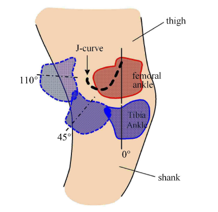
如图 1 所示,人体膝关节由股骨踝 (femoral ankle) 和胫骨踝 (tibia ankle) 组成,依赖于股踝和胫踝接触面的几何外形,人体膝关节的运动属于非定轴转动,小腿相对于大腿转动的速度瞬心轨迹实际是一条 J 形曲线. 其生物学优势在于,在站立相时,膝关节瞬心升高,小腿相对于瞬心的转动惯量较大,不易实现转动,因而稳定性好;反之,在摆动相时,小腿灵活性好,这也是四连杆膝关节仿生学研究的主要动机.

图1

新窗口打开|下载原图ZIP|生成PPT
图1人体膝关节非定轴转动及其 J 形瞬心轨迹

Fig.1Non-fixed axis rotation of human knee joint and its J-curve of instantaneous rotation center

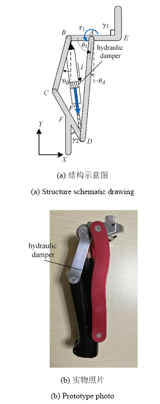
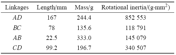
四连杆膝关节可以较好地模拟人体膝关节非定轴转动过程,主要由四根连杆和液压阻尼器组成,其结构示意图及实物图如图 2 所示. 以工道风行公司 (GDFX) 设计的一款四连杆膝关节为例,其几何参数及惯量参数如表 1 所示. 根据四连杆的连接关系,四连杆机构的运动约束方程可以表示为

(1)${\pmb A\pmb B} + {\pmb B\pmb C} + {\pmb C\pmb D} + {\pmb D\pmb A} =0$

在二维笛卡尔坐标系下,式 (1) 可以具体表示为

(2)$\left.\begin{array}{l} \xi _1 : = l_{AB} \sin \left( {\gamma _1 + \alpha _1 } \right) + l_{AD} \sin \theta _A - l_{BC} \sin \theta _B - l_{CD} \sin \left( {\gamma _2 + \alpha _{11} } \right) = 0 \\ \xi _2 : = l_{AB} \cos \left( {\gamma _1 + \alpha _1 } \right) + l_{AD} \cos \theta _A - l_{BC} \cos \theta _B - l_{CD} \cos \left( {\gamma _2 + \alpha _{11} } \right) = 0 \end{array}\!\!\right\}$

其中,$l_{AB} $,$l_{AD} $,$l_{BC} $ 和 $l_{CD} $分别为连杆 $AB$,$AD$,$BC$ 和 $CD$ 的长度,$\gamma _1 = 90^\circ$ 为连杆 $AB$ 与大腿股骨夹角,$\gamma _2 = 24^\circ$ 为连杆 $CD$ 与小腿胫骨夹角,$\theta _A $,$\theta _B $ 分别为连杆 $AD$,$BC$ 与竖直方向夹角,$\alpha _1 $ 为大腿股骨与竖直方向夹角,$\alpha _{11} $ 为小腿股骨与竖直方向夹角.

图2

新窗口打开|下载原图ZIP|生成PPT
图2四连杆膝关节

Fig.2Four-bar linkage prosthesis knee

Table 1
表1
表1四连杆膝关节物理参数表
Table 1Physical parameter values of the four-bar-linkage knee prosthesis

新窗口打开|下载CSV

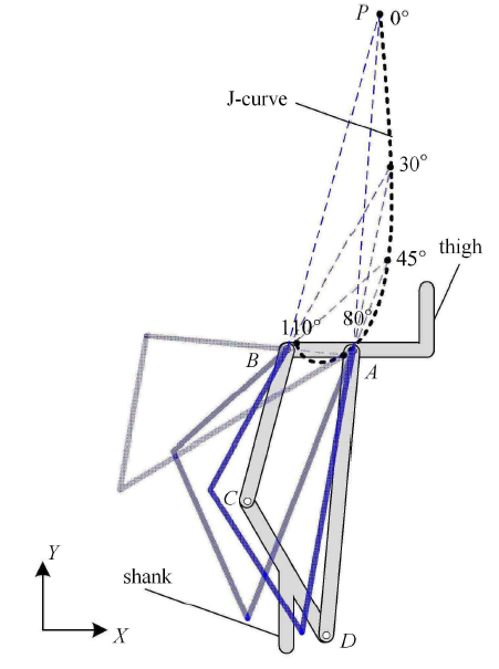
由几何关系可知,四连杆膝关节在转动过程中小腿相对于大腿的瞬心 $P$ 在 $CB$ 和 $DA$ 的延长线上. 在平面笛卡尔坐标系下,瞬心 $P$ 的坐标可以表示为

(3)$\left.\begin{array}{l} x_P = \dfrac{\left( {x_B - x_C } \right)\left( {x_D y_A - x_A y_D } \right)}{\left( {y_A - y_D } \right)\left( {x_B - x_C } \right) - \left( {y_B - y_C } \right)\left( {x_A - x_D } \right)} -\\ \qquad \dfrac{\left( {x_A - x_D } \right)\left( {x_C y_B - x_B y_C } \right)}{\left( {y_A - y_D } \right)\left( {x_B - x_C } \right) - \left( {y_B - y_C } \right)\left( {x_A - x_D } \right)} \\ y_P = \dfrac{\left( {y_B - y_C } \right)\left( {x_D y_A - x_A y_D } \right)}{\left( {y_A - y_D } \right)\left( {x_B - x_C } \right) - \left( {y_B - y_C } \right)\left( {x_A - x_D } \right)} -\\ \qquad \dfrac{\left( {y_A - y_D } \right)\left( {x_C y_B - x_B y_C } \right)}{\left( {y_A - y_D } \right)\left( {x_B - x_C } \right) - \left( {y_B - y_C } \right)\left( {x_A - x_D } \right)} \end{array} \!\! \right \}$

其中,$x_P$ 为瞬心 $P$ 的横坐标,$y_P$ 为瞬心 $P$ 的纵坐标,$x_k $ 和 $y_k $ 分别为四连杆顶点 $k(k = A,B,C,D)$ 的横坐标和纵坐标. 图 3 展示了小腿相对于大腿转动时速度瞬心 $P$ 的轨迹曲线,其中假肢大腿与 $AB$ 杆刚性连接,假肢小腿与 $CD$ 杆刚性连接. 可以看到,在膝关节由伸直状态至 110$^{\circ}$ 屈曲状态过程中,瞬心 $P$ 形成的轨迹是一条 J-curve 线,与人体膝关节瞬心的 J 形轨迹相似,展现了良好的仿生特性.

图3

新窗口打开|下载原图ZIP|生成PPT
图3四连杆膝关节 J 形瞬心轨迹

Fig.3Four-bar linkage prosthesis knee's J-curve of instantaneous rotation center

1.2 足-地交互力和膝关节单边接触力模型

足-地交互作用力主要有地面对假肢足底的接触力和摩擦力两部分. 为方便分析,本文假设只有脚跟和脚尖这两点与地面存在接触力和摩擦力.

地面对足底的接触力可以通过 Kelvin-Voigt 模型来描述

(4)$F_{N,i} = K_{N,i} \delta _i + \chi _{N,i} \dot {\delta }_i$

式中,$F_{N,i}$ 表示接触力,方向垂直于地面,下标 $i$为 heel 或 toe,分别表示脚跟和脚尖与地面接触时接触力的描述. $K_{N,i} $ 表示接触刚度,$\chi _{N,i} $ 表示接触阻尼. $\delta _i $ 表示脚尖或脚跟与地面之间的压痕深度,当脚尖或脚跟离地时,规定 $\delta _i = 0$. 地面对足底的摩擦力采用库伦摩擦模型描述^[16]

(5)$F_{f,i} = -{\rm sgn} \left( {v_i } \right)\mu F_{N,i}$

式中,$F_{f,i} $ 表示摩擦力,方向沿水平方向,下标 $i$ 为 heel 或 toe,分别表示脚跟和脚尖与地面接触时摩擦力的描述. $\mu $ 表示动摩擦系数 (此处忽略静摩擦系数),$v_i $ 表示脚尖或脚跟相对地面的切向速度.为方便动力学分析,本文对式 (4) 所述接触力模型和式 (5) 所述摩擦力进行光滑化处理,具体光滑化形式分别为

(6)$F_{N,i} = \left[ {\dfrac{1}{2} - \dfrac{\arctan \left( {C_1 \delta _i } \right)}{\pi }} \right]\left( {K_{N,i} \delta _i + \chi _{N,i} \dot {\delta }_i } \right)$

(7)$F_{f,i} = - \dfrac{2\arctan \left( {C_2 v_i } \right)}{\pi }\mu F_{N,i}$

其中 $C_1 $ 和 $C_2 $ 为常数,表征接触力和摩擦力的光滑化程度.

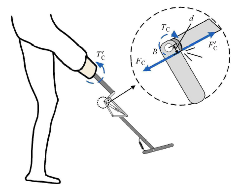
此外,如图 4 所示,当假肢小腿摆动到与大腿呈同一角度时 (即膝关节打直),为保证穿戴者安全性,四连杆的 $AB$ 和 $BC$ 两杆之间将通过限位装置锁死,锁死端面垂直于$AB$连杆. 这种结构锁死是一种单边约束,力学上可以简化为单边接触模型. 因此,本文同样通过光滑化的 Kelvin-Voigt 模型来描述膝关节打直的单边接触力,具体形式为

(8)$F_{\rm c} = \left[ {\dfrac{1}{2} - \dfrac{\arctan \left( {C_3 \delta _{\rm knee} } \right)}{\pi }} \right]\left( {K_{\rm c} \delta _{\rm knee} + C_{\rm c} \dot {\delta }_{\rm knee} } \right)$

图4

新窗口打开|下载原图ZIP|生成PPT
图4膝关节几何锁死时接触力示意图

Fig.4The contact force when the knee is locked geometrically

其中,$F_{\rm c}$ 表示单边接触力,方向为 $AB$ 连杆方向,$K_{\rm c}$ 表示接触刚度,$C_{\rm c}$ 表示接触阻尼,$\delta _{\rm knee}$ 表示两杆之间的压痕深度. 需要注意的是,如图 4 中细节放大图所示, $AB$ 和 $BC$ 两杆间限位接触点与 $B$ 点不重合,其偏心距为 $d = 1$cm,因此式 (8) 所示接触力作用于连杆 $BC$ 和 $AB$ 的力矩分别为

(9)$T_{\rm c}= F_{\rm c} d, \ \ {T}'_{\rm c} = - T_{\rm c}$

至此,本文得到了足-地交互作用力和膝关节单边接触力的模型.

1.3 基于第一类拉格朗日方程的动力学建模

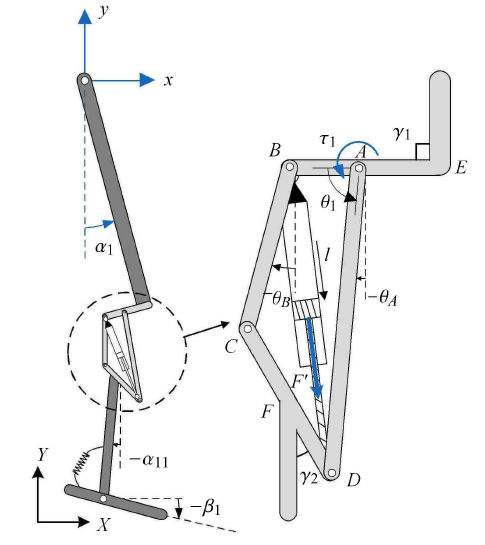
假设四连杆膝关节的接受腔与残疾人大腿残肢为刚性连接,因此四连杆膝关节被动假肢的运动模型可简化为图 5 所示形式. 其中 $x$ 和 $y$ 分别为髋关节在平面笛卡尔坐标系下的横坐标和纵坐标,$\alpha _1 $ 为大腿与竖直方向的夹角,$\alpha _{11} $ 为小腿与竖直方向夹角,$\beta _1 $ 为足部与水平方向夹角.

图5

新窗口打开|下载原图ZIP|生成PPT
图5四连杆膝关节被动假肢运动模型

Fig.5Model of passive four-bar linkage prosthesis knee

如图 5 所示,四连杆机构中的液压阻尼器主要是在运动过程中提供阻尼力和回复力,其合力可以表示为

(10)${F}' = - k\left( {l - l_0 } \right) - c\dot {l}$

式中,$k$ 和 $c$ 分别为液压阻尼器的刚度和阻尼系数,$l_0 = 168.79$mm 为液压阻尼器原长,$l$ 为当前长度. 基于虚功原理,合力 ${F}'$ 作用于广义坐标 $\theta _1 $ 上的广义力为

(11)$\tau _1 = F'\dfrac{\text{d}l}{\text{d}\theta _1 } = \dfrac{F'l_{AD} l_{AB} \sin \theta _1 }{\sqrt {l_{AD} ^2 + l_{AB} ^2 - 2l_{AD} l_{AB} \cos \theta _1 } }$

此外,由于 $\theta _1 = 0.5\pi - \alpha _1 + \theta _A $,因此合力 ${F}'$ 作用于广义坐标 $\alpha _1 $ 和 $\theta _A $ 上的广义力矩分别为 $ - \tau _1 $ 和 $\tau _1 $.

此外,本文假设踝关节受到带阻尼的扭簧作用,作用力矩表示为

(12)$T_{\rm ankle} = - k_{\rm ankle} \left( {\varphi _{\rm ankle} - \varphi _0 \left( t \right)} \right) - c_{\rm ankle} \dot {\varphi }_{\rm ankle}$

其中,$k_{\rm ankle} = 10$N/m 和 $c_{\rm ankle} = 0.2$N/(m$\cdot$s$^{ - 1}$) 分别为扭簧的刚度和阻尼系数,$\varphi _{\rm ankle} $ 为踝关节角度,$\phi _0 \left( t \right)$ 为踝关节期望角度.在步态分析中,本文以实测踝关节角度作为 $\varphi _0 \left( t \right)$. 由图 5 可知,踝关节角度 $\varphi _{\rm ankle} $ 满足 $\varphi _{\rm ankle} = \beta _1 - \alpha _{11} $,因此扭簧作用于广义坐标 $\alpha _{11} $ 和 $\beta _1 $ 的扭矩分别为 $ - T_{\rm ankle} $ 和 $T_{\rm ankle} $.

得到基于四连杆约束的运动学模型、足-地交互力和膝关节单边接触力模型后,图 5 所示的四连杆膝关节被动假肢的动力学模型可以用第一类拉格朗日方程表示

(13)${\pmb M}\ddot {q} + {\pmb C}\dot {q} +{\pmb N} = {\pmb F}_{\rm e} + {\pmb F}_{\rm q} + {\pmb \Phi }^{\rm T}{\pmb \lambda }$

式中,${\pmb q} = \left( {x,y,\alpha _1 ,\alpha _{11} ,\theta _A ,\theta _B ,\beta _1 } \right)^ {\rm T}$ 为广义坐标向量,${\pmb M}\left( {\pmb q} \right) \in \mathbb{R}^{7\times 7}$ 是质量阵,${\pmb C} \left( {{\pmb q},\dot{\pmb q}} \right) \in \mathbb{R}^{7\times 7}$ 是科氏力和离心力项,${\pmb N}\left( {\pmb q} \right) \in \mathbb{R}^{7\times 1}$ 是重力项. ${\pmb M}\left( {\pmb q} \right)$, ${\pmb C}\left( {{\pmb q},\dot{\pmb q}} \right)$ 及 ${\pmb N}\left( {\pmb q} \right)$ 中各元素表达式见附录 A. ${\pmb F}_{\rm e} $ 为足-地交互作用力和膝关节单边接触力构成的广义力向量,具体表示为

(14)${\pmb F}_{\rm e} = {\pmb J}^{\rm T}\left( {F_{\rm N,heel} , F_{\rm N,toe} , F_{\rm f,heel} , F_{\rm f,toe} , T_{\rm c}, {T}'_{\rm c} } \right)^ {\rm T}$

其中,$F_{\rm N,heel} $ 和 $F_{\rm N,toe} $ 由式 (6) 给出,$F_{\rm f,heel} $ 和 $F_{\rm f,toe} $ 由式 (7) 给出,$T_{\rm c}$ 和 ${T}'_{\rm c}$ 由式 (9) 给出,${\pmb J}$ 为将足-地交互作用力和膝关节单边接触力变换为广义力的 Jacobi 矩阵,具体形式见附录 A. ${\pmb F}_q $ 为膝关节的液压阻尼器和踝关节的阻尼弹簧施加的广义力向量,具体表示为

(15)${\pmb F}_{\rm q} = \left( {0, 0, - \tau _1 , - T_{\rm ankle} , \tau _1 , 0, T_{\rm ankle} } \right)^ {\rm T}$

其中,$\tau _1 $ 由式 (11) 给出,$T_{\rm ankle} $ 由式 (12) 给出. ${\pmb \varPhi }$ 为四连杆约束矩阵,具体表示为

(16)${\pmb \varPhi } = \dfrac{\partial {\pmb \xi }\left( {\pmb q} \right)}{\partial {\pmb q}^{\rm T}} = \dfrac{\partial \left( {\xi _1 , \xi _2 } \right)^{\rm T}}{\partial {\pmb q}^{\rm T}}$

其中,$\xi _1 $ 和 $\xi _2 $ 为式 (2) 所示约束方程. ${\pmb \lambda }$ 为拉格朗日乘子,表示四连杆约束产生的约束力.

需要指出的是,被动假肢是由髋关节运动驱动的,髋关节运动信号 $x$,$y$,$\alpha _1 $ 为假肢系统的输入,$\alpha _{11} $,$\theta _A $,$\theta _B $ 和 $\beta _1 $ 为假肢系统的响应. 为方便步态分析,式 (13) 可以改写为

(17)${\pmb M}_2 \ddot{\pmb q}_2 + {\pmb C}_2 \dot {\pmb q}_2 + {\pmb N}_2 ={\pmb F}_{\rm e2} + {\pmb F}_{\rm q2} - {\pmb M}_1 \ddot {\pmb q}_1 - {\pmb C}_1 \dot{\pmb q}_1 + {\pmb \varPhi }_2 ^{\rm T}{\pmb \lambda } $

其中

$ {\pmb q}_1 = \left( {x, y, \alpha _1 } \right)^{\rm T}, \ \ {\pmb q }_2 = \left( {\alpha _{11} , \theta _A , \theta _B , \beta _1 } \right)^{\rm T} \\ {\pmb M} = \left(\!\! \begin{array}{cc} {\pmb M}_{\rm e1} & {\pmb M}_{\rm e2} \\ {\pmb M}_1 & {\pmb M}_2 \\ \end{array}\!\! \right), \ \ {\pmb M}_{1} \in \mathbb{R}^{4\times 3}, \ \ {\pmb M}_2 \in \mathbb{R}^{4\times 4} \\ {\pmb C} = \left(\!\! \begin{array}{cc} {\pmb C}_{\rm e1} & {\pmb C}_{\rm e2} \\ {\pmb C}_1 & {\pmb C}_2 \end{array}\!\! \right), \ \ {\pmb C}_1 \in \mathbb{R}^{4\times 3}, \ \ {\pmb C}_2 \in \mathbb{R}^{4\times 4} \\ {\pmb N} = \left(\!\! \begin{array}{c} {{\pmb N}_{\rm e} } \\ {{\pmb N}_2 } \end{array}\!\! \right), \ \ {\pmb N}_2 \in \mathbb{R}^{4\times 1}, \ \ {\pmb F}_{\rm e} = \left(\!\! \begin{array}{c} {\pmb F}_{\rm e1} \\ {\pmb F}_{\rm e2} \end{array}\!\! \right), \ \ {\pmb F}_{\rm e2} \in \mathbb{R}^{4\times 1} \\ {\pmb F}_{\rm q} = \left(\!\! \begin{array}{c} {\pmb F}_{\rm q1} \\ {\pmb F}_{\rm q2} \end{array}\!\! \right), \ \ {\pmb F}_{\rm q2} \in \mathbb{R}^{4\times 1}, \ \ {\pmb \varPhi } = \left(\!\! \begin{array}{c} {\pmb \varPhi}_1 ^{\rm T} \\ {\pmb \varPhi}_2 ^{\rm T} \end{array} \!\! \right)^{\rm T}, \ \ {\pmb \varPhi }_2 \in \mathbb{R}^{2\times 4} $

对于 ${\pmb \lambda }$ 的具体形式,因为 $\dot {\xi }_1 = \dot {\xi }_2 =0$,即

(18)$\left( {\dot {\xi }_1 , \dot {\xi }_2 } \right)^{\rm T} = \dfrac{\partial \left( {\xi _1 , \xi _2 } \right)^ {\rm T}}{\partial {\pmb q }^{\rm T} }\dot{\pmb q} = {\pmb \varPhi}_1 \dot{\pmb q }_1 + {\pmb \varPhi }_2 \dot{\pmb q}_2 = 0$

将式 (18) 对时间 $t$ 求导可得

(19)${\pmb \varPhi }_2 \ddot{\pmb q}_2 + {\pmb \varPhi }_1 \ddot {\pmb q}_1 + \dot{\pmb \varPhi}_2 \dot{\pmb q}_2 + \dot {\pmb \varPhi}_1 \dot{\pmb q}_1 = 0$

代入式 (17) 可得

(20)$\ddot{\pmb q}_2 = {\pmb M}_2 ^{ - 1}\left( {{\pmb F}_{\rm e} + {\pmb F}_{\rm q} + {\pmb \varPhi }_2 ^{\rm T}{\pmb \lambda }} \right) -\\ \qquad {\pmb M}_2 ^{ - 1}\left( {{\pmb M}_1 \ddot{\pmb q}_1 + {\pmb C}_1 \dot{\pmb q}_1 + {\pmb C}_2 \dot {\pmb q}_2 + {\pmb N}_2 } \right)$

进一步,将式(20)代入式(19)可解得

(21)${\pmb \lambda } = \left( {{\pmb \varPhi }_2 {\pmb M}_2 ^{ - 1}{\pmb \varPhi }_2 ^T} \right)^{ - 1} \left( { - {\pmb \varPhi }_1 \ddot {\pmb q}_1 - \dot{\pmb \varPhi}_2 \dot{\pmb q}_2 - \dot{\pmb \varPhi}_1 \dot{\pmb q}_1 } \right) +\\ \qquad \left( {{\pmb \varPhi}_2 ^T} \right)^{ - 1}\left( {{\pmb C}_2 \dot{\pmb q}_2 + {\pmb N}_2 - {\pmb F}_{\rm e} - {\pmb F}_{\rm q} + {\pmb M}_1 \ddot {\pmb q}_1 + {\pmb C}_1 \dot {\pmb q}_1 } \right)$

令

${\pmb x}_1 = \left(\begin{array}{c} {\pmb q}_1 \\ \dot{\pmb q}_1 \end{array} \right), \ \ {\pmb x}_2 = \left(\begin{array}{c} {\pmb q}_2 \\ \dot{\pmb q}_2 \end{array} \right)$

式(17)可以改写为如下状态方程形式

(22)$\dot{\pmb x}_2 = {\pmb f}\left( {{\pmb x}_2 ,{\pmb x}_1 ,\dot{\pmb x}_1 } \right) + {\pmb g}\left( {{\pmb x}_2 ,{\pmb x}_1 ,\dot{\pmb x}_1 } \right){\pmb \lambda }$

其中

$ {\pmb f}\left( {{\pmb x}_2 ,{\pmb x}_1 , \dot {\pmb x}_1 } \right) = \left(\!\!\begin{array}{c} \dot{\pmb q}_2 \\ {\pmb M}_2 ^{ - 1}\left( {{\pmb F}_{\rm e} + {\pmb F}_{\rm q} - {\pmb M}_1 \ddot{\pmb q}_1 - {\pmb C}_1 \dot{\pmb q}_1 - {\pmb C}_2 \dot{\pmb q}_2 - {\pmb N}_2 } \right) \end{array}\!\! \right) \\ {\pmb g}\left( {{\pmb x}_2 ,{\pmb x}_1 } \right) = \left(\!\!\begin{array}{c} 0 \\ {\pmb M}_2 ^{ - 1}{\pmb \varPhi }_2 ^{\rm T} \end{array} \!\! \right) $

至此,我们得到了考虑四连杆约束、足-地交互力和膝关节单边接触力的四连杆膝关节被动假肢的动力学模型. 如前所述,被动假肢是由髋关节运动驱动的,髋关节运动信号 ${\pmb q}_1 = \left( {x,y,\alpha _1 } \right)^{\rm T}$ 及其速度 $\dot {\pmb q}_1 $ 和加速度 $\ddot {\pmb q}_1 $ 为式 (22) 的输入. 后续,在基于该模型的动力学分析中,${\pmb q}_1 $ 为健康被试的实测运动信号.

2 健康被试的步态测试

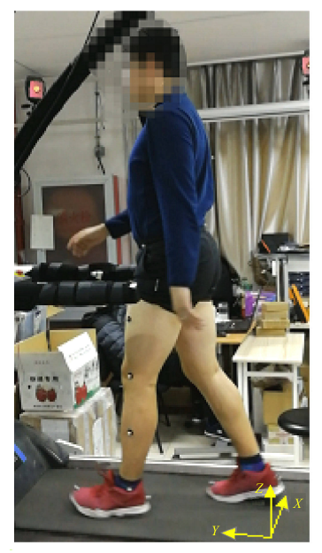
该人体步态测试实验已获得北京大学伦理委员会批准.实验目的在于：第一,获得式 (22) 右端所需要的输入 ${\pmb q}_1 $,$\dot{\pmb q}_1 $,$\ddot {\pmb q}_1 $,用于四连杆膝关节被动假肢的动力学仿真;第二,将健康被试的步态信号作为健肢步态信号,与动力学仿真所得假肢步态进行比较,用于假肢运动与健肢运动的步态分析.

实验所用设备为 Cosmos Gaitway 跑台和 Vicon 光学运动捕捉系统及配套分析系统. 其中,Cosmos Gaitway 跑台用于实现匀速步行环境,Vicon 光学运动捕捉系统用于捕捉人体靶点运动信号,并换算为各关节角度信息. 参考步态分析软件 OrthoTrak 用户指南中的 Helen-Hayes 模型,健康被试身共贴有 18 个靶点,分别为右肩靶点 (R. shoulder)、左肩靶点 (L. shoulder)、补偿靶点 (offset)、左髂前上棘靶点 (R. asis)、右髂前上棘靶点 (L. asis)、骶骨靶点 (V. sacral)、右大腿靶点 (R. thigh)、左大腿靶点 (L. thigh)、右膝靶点 (R. knee)、左膝靶点 (L. knee)、右小腿靶点 (R. shank)、左小腿靶点 (L. shank)、右脚跟靶点 (R. heel)、左脚跟靶点 (L. heel)、右脚踝靶点 (R. ankle)、左脚踝靶点(L. ankle)、右脚尖靶点 (R. toe) 和左脚尖靶点 (L. toe). 步态测试实景如图 6 所示,图中 $Y$ 轴沿着被试行走正前方,$X$ 轴沿着被试行走侧向,$Z$ 轴沿着竖直向上方向. 实验过程中,健康被试 (男性,身高 182cm,体重 92kg) 在 Cosmos Gaitway 跑台上行走 (坡度 0,速度 1m/s),Vicon 光学运动捕捉系统采样频率为 100Hz,采样时长 180s.

图6

新窗口打开|下载原图ZIP|生成PPT
图6健康被试步态测试过程

Fig.6Able-bodied subject test process

实验最终得到的数据是各靶点的空间坐标,采用 Helen-Hayes 模型的角度解算方法可以得到髋关节处的空间坐标和髋、膝、踝关节的空间转角^[33]. 式 (22) 所示动力学模型为平面模型,根据坐标对应关系,本文取图 6 中髋关节处的 $Y$ 轴坐标和 $Z$ 轴坐标分别作为广义坐标 ${\pmb q}$ 中 $x$,$y$ 坐标,取各关节绕 $X$ 轴方向的转角作为广义坐标 ${\pmb q}$ 中的 $\alpha _1 $,$\alpha _{11} $,$\beta _1 $ 坐标.

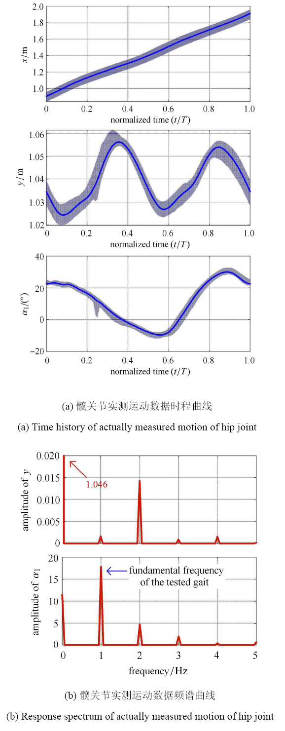
为使实验数据反映健康人步态的普遍规律,本文以两次脚跟着地 (heel strike,HS) 之间的时间间隔作为一个步态周期 $T$,选取实验数据中的 30 个周期进行平均,同时将时间归一化. 处理后得到的 ${\pmb q}_1 $ 数据如图 7 所示. 图 7(a) 中的蓝色实线表示平均后的 ${\pmb q}_1 $ 时程,阴影部分的上下界分别表示 30 个周期中各个时刻点的最大值和最小值. 从阴影部分的面积可以看出,各周期步态较为一致,实验结果较为可靠,因此取 30 个周期进行平均是合理的,能够准确地反映 ${\pmb q}_1 $ 广义坐标的运动特征. 图 7(b) 中展示了广义坐标 $y$ 和 $\alpha _1 $ 的频谱图 (广义坐标 $x$ 的运动不具有周期性,因此无需进行频谱分析). 可以看到,$y$ 信号中 2Hz 频率成分的振幅较大,这是因为健康被试在一个步态周期中,左腿和右腿各走了一步,导致髋关节在竖直方向呈现两次近似相同的起伏;$\alpha _1 $ 信号中 1Hz频率成分的振幅较大,这一点并不难理解. 上述分析可以说明输入信号 ${\pmb q}_1 $ 的激励频率为 1Hz,这为第 3 中对系统响应的分析奠定基础.

图7

新窗口打开|下载原图ZIP|生成PPT
图7髋关节实测运动数据时程和频谱曲线

Fig.7Time history and response spectrum of actually measured motion of hip joint

此外,式 (22) 的输入信号还包含 $\dot{\pmb q}_1 $ 和 $ \ddot {\pmb q}_1 $. 为此,本文首先对实测信号 ${\pmb q}_1 $ 进行傅里叶级数拟合,进而对拟合得到的函数分别求一阶导和二阶导得到 $\dot{\pmb q}_1 $ 和 $ \ddot{\pmb q}_1 $,以最大程度避免实测信号中噪声的放大.

3 四连杆被动假肢的步态分析

基于式 (22) 并以第 2 节的实验数据作为输入,对四连杆膝关节假肢进行动力学仿真,仿真所采用的物

理参数如表 2 所示. 足-地交互作用力和膝关节单边接触力的模型参数如下

$ K_{\rm N} = 1.0\times 10^5{\rm N / m}, \ \ \chi _{\rm N} = 20{\rm N}/ ({\rm m}\cdot {\rm s}^{- 1} ) , \ \ \mu = 0.6 \\ K_{\rm c} = 7.5\times 10^4{\rm N / m}, \ \ C_{\rm c} = 20{\rm N}/ ({\rm m}\cdot {\rm s}^{- 1} ) \\ C_1 = 1.0\times 10^6, \ \ C_2 = 1.0\times 10^4, \ \ C_3 = 1.0\times 10^6 $

Table 2
表2
表2仿真中的部分物理参数值
Table 2Physical parameters in numerical simulation

新窗口打开|下载CSV

为保证仿真所得数据为假肢的稳态响应,仿真时长设置为 20 个步态周期,取末 5 个步态周期用于分析.

3.1 亚谐波频率响应

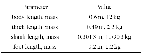
动力学仿真中,设置液压阻尼器阻尼/刚度比为 $c / k = 0.05$,刚度系数分别为 $k = 1.4\times 10^4$N/m和 $k = 1.52\times 10^4$N/m. 图 8(a) 展示了健康被测的实测步态数据及基于动力学模型的仿真数据,其中纵坐标定义为 $\phi_{\rm knee} = \alpha _1 - \alpha _{11} $. 则从图 8(a) 阴影部分可以看出,当 $k = 1.4\times 10^4$N/m 时,四连杆膝关节被动假肢的动力学仿真响应的周期为 $2 T$;当 $k =1.52\times 10^4$N/m,动力学仿真响应的周期为 $3 T$.

图8

新窗口打开|下载原图ZIP|生成PPT
图8亚谐波响应时程曲线与频谱曲线

Fig.8Time history and response spectrum of subharmonic response

进一步地,我们对动力学响应信号进行FFT频谱分析. 图 8(b) 展示了对应于两个时间历程的频谱图.

图 8(b) 表明,当 $k \!=\!1.4\times 10^4$N/m 时,主要的频率成分为 1Hz 和 2Hz,同时出现了 1/2Hz 频率成分,这一亚谐频率成分使得响应的周期为 $2 T$;当 $k = 1.52\times 10^4$N/m 时,主要频率成分仍为 1Hz 和 2Hz,同时出现了 1/3Hz 频率成分,这一亚谐频率成分使得响应的周期为 $3 T$.这些亚谐波频率成分出现的原因在于,足-地交互作用力和膝关节单边接触力含有强非线性因素,可以诱发四连杆被动假肢的亚谐波响应这一强非线性动力学行为. 1/2 或 1/3 亚谐波响应表明,此时假肢的步态周期为健肢步态周期的 2 倍或 3 倍,破坏了行走时双腿步态的协调性,本文将这种亚谐波响应称为步态周期失谐.

通过进一步的非线性动力学分析,我们发现,通过调整激励参数 (如初始条件、相位、幅值等),系统的稳态响应可以切换回单周期状态. 反映到式 (22) 所示的四连杆膝关节被动假肢模型中,即表现为髋关节运动信号的调整.

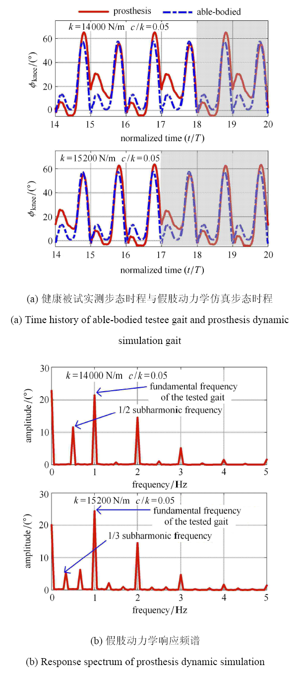
例如,图 9(a) 和图 9(b) 分别展示了将髋关节竖向运动信号 $y$ 放大为原信号 1.006 倍后假肢膝关节角度的时程曲线和频谱曲线.

图9

新窗口打开|下载原图ZIP|生成PPT
图9提胯后响应时程曲线与频谱曲线

Fig.9Time history and response spectrum when lifting the hip

从图 9(a) 可以看出,在增大髋关节竖向运动幅值后,假肢响应在两个刚度值下均达到单周期稳态,周期和实测数据相同为 $T$,并与实测数据有较好的步态一致性. 图 9(b) 表明,假肢的亚谐波频率成分消失,其基频与健肢的基频相同,为 1Hz,步态周期不再失谐.

放大髋关节竖向运动信号所反映的生物意义类似于提胯,即残疾人在运动过程中提高胯部动作幅度的行为. 图 9 呈现的结论说明,提胯动作将改善假肢步态周期的协调性,使步态不再失谐,这在定性上解释了残疾人穿戴假肢行走时会出现提胯等代偿动作产生的原因.

注意到,在式 (22) 所示的四连杆膝关节被动假肢动力学模型中,四连杆的几何参数、模型所受激励信号均是基于实验实测所得,因而所得结果具有较高的可信度. 但上述亚谐波频率成分和亚谐波响应,尚未在四连杆膝关节的研究文献中见到相关报道.

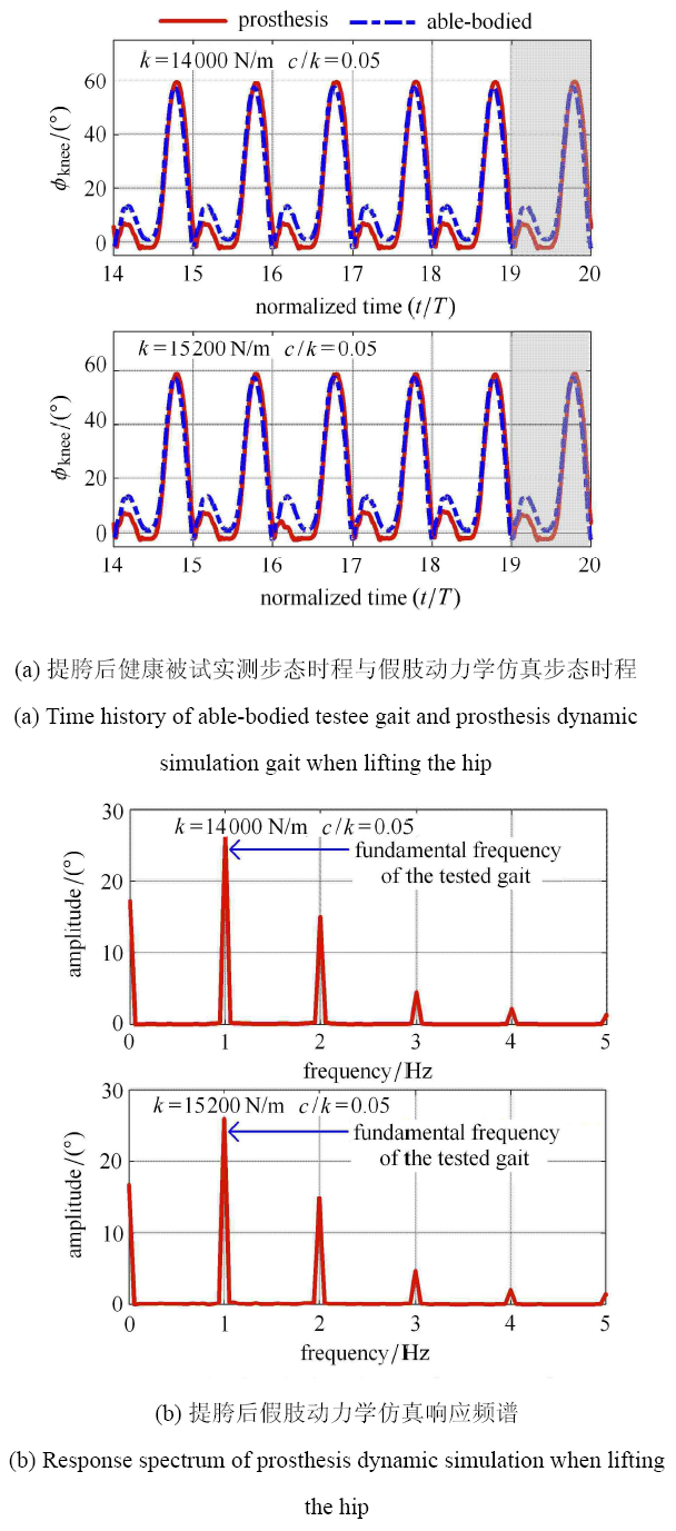
数值分析进一步发现,保持四连杆膝关节液压阻尼器阻尼比值不变,在 $k$ 值达到 1.6$\times$10$^4$N/m 以上时,亚谐波频率响应基本消失,假肢膝关节的运动恢复为单周期的稳态解,因此将 $k = 1.6\times 10^4$N/m 称为此时的临界 $k$ 值. 图 10 展示了 $k = 1.6\times 10^4$N/m 时假肢动力学仿真时程和响应频谱,显见假肢响应达到了单周期稳态,且周期与实测数据相同.

图10

新窗口打开|下载原图ZIP|生成PPT
图10单周期稳态下假肢动力学仿真步态时程和响应频谱

Fig.10Time history and response spectrum of prosthesis dynamic simulation gait under uniperiodic steady state

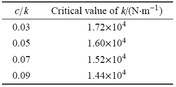
图 11 给出了 $c / k \!=\!0.05$ 时各个刚度值下膝关节的时程响应的频谱图. 可以看到,在刚度值在 (1.4$\sim $1.65)$\times$10$^4$N/m 变化的过程中,响应在红色区域 (1.45$\sim $1.47)$\times$10$^4$N/m 出现了持续且显著的1/2 亚谐波频率成分,在 (1.47$\sim $1.5)$\times$10$^4$N/m 进入多亚谐波频率成分混杂的阶段,在蓝色区域 (1.5$\sim $ 1.56)$\times$10$^4$N/m 出现了持续且显著的 1/3 亚谐波频率成分,随后各亚谐波频率成分逐渐减少并进入单一稳态阶段 (1.56 $\sim $ 1.65)$\times$10$^4$N/m. 另外值得注意的是,在 (1.4 $\sim $ 1.45)$\times$10$^4$N/m 阶段,响应在 (1.4 $\sim $ 1.42)$\times$10$^4$N/m 时出现了 1/2 亚谐波频率成分,而在 (1.42 $\sim $ 1.45)$\times$10$^4$N/m 时出现多亚谐波频率成分混杂的情况,这一部分值得在之后的研究中进一步探讨. 根据以上分析,可以认为在刚度值增大到一定程度时,亚谐波频率成分会消失,将亚谐波频率成分完全消失时的 $k$ 值叫作临界 $k$ 值,并在表 3 中给出了其他 $c / k$ 值下的临界 $k$ 值.

图11

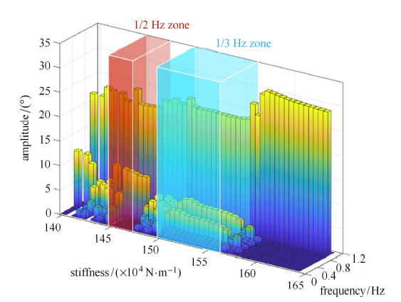新窗口打开|下载原图ZIP|生成PPT
图11不同刚度值下假肢膝关节频率响应图

Fig.11Response spectrum of prosthesis knee under different values of stiffness

Table 3
表3
表3临界 $k$ 值
Table 3Critical value of $k$

新窗口打开|下载CSV

分析表 3 可以发现,阻尼比值越大,单周期稳态解对应的临界 $k$ 值越低. 这表明,可以通过适当调大四连杆膝关节液压阻尼器的阻尼、刚度系数来改善假肢步态周期的协调性.

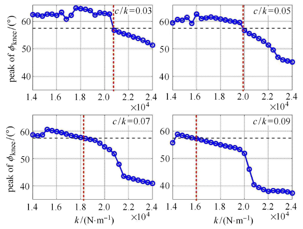
3.2 假肢膝关节最大屈曲角度

膝关节最大屈曲角指每个步态周期内 $\phi _{\rm knee} $ 的最大值,图 10 中标注为 peak of $\phi _{\rm knee} $,它直接反映了足部最大离地间隙,是评价假肢穿戴安全性的重要指标之一. 图 12 展示了不同阻尼比值下膝关节最大屈曲角随液压阻尼器刚度系数的变化关系,其中蓝色圆圈表示的是数值计算所得最大屈曲角,黑色虚线表示的是健康被试实测最大屈曲角.

图12

新窗口打开|下载原图ZIP|生成PPT
图12不同阻尼比值下膝关节最大屈曲角

Fig.12Peak of knee angle under different damping ratios

可以看出,随着 $k$ 值增大,膝关节最大屈曲角度呈现递减趋势. 同时可以看出,随着阻尼比值的增大,假肢膝关节最大屈曲角与实测膝关节最大屈曲角相等时所对应的刚度值 $k$ (红色竖直虚线所对应的 $k$ 值) 也呈现递减规律. 这表明,若调大膝关节液压阻尼器的阻尼、刚度系数,尽管假肢步态周期的协调性能够得到改善,但假肢膝关节的最大屈曲角却有可能偏离最优值. 因此,未来的工作中,我们有必要选择或定义合理的步态协调性指标,以便对四连杆膝关节假肢进行优化.

3.3 假肢与健肢膝关节步态一致性

为了定量衡量假肢与健肢步态的一致性,本文定义假肢与健肢膝关节信号的相关系数 (correlation coefficient),计算公式如下

(23)$\rho _{XY} = \dfrac{{\rm Cov}\left( {X, Y} \right)}{\sqrt {D\left( X \right)} \sqrt {D\left( Y \right)} }$

其中

$ {\rm Cov} \left( {X, Y} \right) = \dfrac{T}{ t_2 - t_1 }\int_{t_1 / T}^{t_2 / T} {XY \text{d}t} - \left( {\dfrac{T}{ t_2 - t_1 }\int_{t_1 / T}^{t_2 / T} {X \text{d}t} } \right)\left( {\dfrac{T}{ t_2 - t_1 }\int_{t_1 / T}^{t_2 / T} {Y \text{d}t} } \right) \\ D\left( X \right) = \dfrac{T}{ t_2 - t_1 }\int_{t_1 / T}^{t_2 / T} {X^2 \text{d}t} - \left( {\dfrac{T}{ t_2 - t_1 }\int_{t_1 / T}^{t_2 / T} {X\text{d}t} } \right)^2 \\ D\left( Y \right) = \dfrac{T}{ t_2 - t_1 }\int_{t_1 / T}^{t_2 / T} {Y^2 \text{d}t} - \left( {\dfrac{T}{ t_2 - t_1 }\int_{t_1 / T}^{t_2 / T} {Y \text{d}t} } \right)^2 $

式中 $X = \alpha _1 - \alpha _{11} $ 为动力学仿真所得膝关节角度信号,$Y$ 为健康被试实测膝关节角度信号,$ {\rm Cov} \left( {X, Y} \right)$为 $X$ 和 $Y$ 信号的协方差,$D ( X )$ 和 $D ( Y )$ 分别为 $X$ 和 $Y$ 信号的方差,$t_1 / T$ 和 $t_2 / T$ 分别为 15 和 20. 理论上,$0 \leqslant \rho _{XY} \leqslant 1$,$\rho _{XY} $ 越大,表示假肢膝关节角度信号与健肢膝关节角度信号一致性越高. 当且仅当 $X\equiv Y$ 时,$\rho _{XY} = 1$.

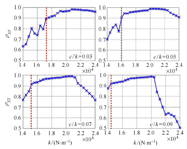
图 13 展示了不同的 $c / k$ 值下 $\rho _{XY} $ 随液压阻尼器刚度的变化. 可以看出,在 $c / k$ 较小 ($c / k = 0.03$, 0.05) 且 $k$ 较小时,$\rho _{XY} $ 呈现抖动的状态,这是因为,此时假肢的响应出现亚谐波频率成分,导致 $\rho _{XY} $ 出现极小值点,呈现抖动的状态. 根据 3.1 节的分析可知,$k$ 在超过一定值时,假肢响应会转变为单周期稳态响应,图 13 中已根据表 3 标出临界 $k$ 值 (红色竖直虚线所对应的 $k$ 值). 在达到临界$k$值后,$\rho_{XY} $ 呈现先增大后减小的规律性变化. 这进一步验证了 3.1 节所述临界$k$值的合理性.

图13

新窗口打开|下载原图ZIP|生成PPT
图13不同阻尼比值下假肢-健肢膝关节相关系数

Fig.13Prosthesis-intact knee joint correlation coefficient under different damping ratios

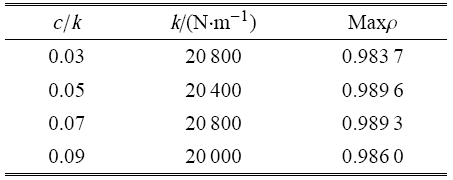
在转变为单周期稳态响应之后,在不同的$c / k$ 下,随着 $k$ 增大,$\rho _{XY} $ 均呈现先增大后减小的规律,因此 $\rho _{XY} $ 存在一个最大值点. 这表明我们可以通过四连杆膝关节液压阻尼器阻尼、刚度参数的设计,对假肢的步态一致性进行优化. 表 4 反映了不同液压阻尼器阻尼比值设置下,最大相关系数 $\rho _{XY} $ 及其对应的液压阻尼器刚度值. 可以看出,在不同的液压阻尼器阻尼比值下,最大相关系数的值均相近,且最大可得到 0.9896,这为设计液压阻尼器的刚度和阻尼值提供了一定的理论依据.

Table 4
表4
表4最大相关系数及对应液压阻尼器刚度
Table 4Max $\rho$ and its corresponding hydraulic damper stiffness

新窗口打开|下载CSV

同时可以发现,随着 $c / k$ 增大,$\rho _{XY} $ 在达到最大值后的下降速度增大. 因此可以发现,$c / k$ 越小,$\rho _{XY} $ 越能在一个较大的$k$范围内保持平缓的变化. 这表明,为了使假肢与健肢在较大的$k$值范围内达到较好的步态一致性,$c / k$ 不宜取得过大.

以上分析表明,为了实现最好的步态一致性,可以通过单目标优化方法找到最合适的 $k$ 值和 $c$ 值. 另外,也可以围绕着步态一致性探究一些多目标优化问题,如为了实现在较大的 $k$ 值范围内达到较好的步态一致性,通过多目标优化方法找到最合适的 $c / k$ 值.关于这部分的研究工作可以在后续展开.

4 结论

本文以一款四连杆膝关节假肢为研究对象,考虑足-地交互作用力和膝关节单边接触力等强非线性因素,采用光滑化的 Kelvin-Voigt 接触模型和库伦摩擦模型描述足-地接触力和摩擦力,采用光滑化的 Kelvin-Voigt 接触模型描述膝关节单边接触力,并基于第一类拉格朗日方程对四连杆膝关节被动假肢进行动力学建模,得到了考虑足-地交互作用力和膝关节单边接触力的一体化假肢动力学模型. 本文将假肢动力学仿真结果与健康被试实测结果对比,系统分析了假肢动力学响应与四连杆膝关节液压阻尼器的刚度、阻尼参数与假肢动力学响应和步态评价指标之间的关系. 通过本文的研究,主要结论如下：

(1) 考虑足-地交互作用力、单边接触力等强非线性因素后,假肢的动力学响应呈现出丰富的非线性现象,如出现了 1/2 和 1/3 亚谐波频率,这种现象破坏了行走时双腿步态的协调性. 在髋关节运动中加入提胯动作后,假肢的动力学响应中的亚谐波频率成分消失,转变为单周期稳态响应,这为残疾人行走时提胯等代偿行为的提供了一种新的力学解释.

(2) 假肢膝关节液压阻尼器刚度 $k$ 和阻尼 $c$ 对膝关节最大屈曲角度有影响. 通过减小刚度 $k$ 和阻尼 $c$ 可以增大膝关节最大屈曲角,这有利于增大足部离地间隙,进而提高运动安全性,但过低的刚度有可能导致步态失谐,从另一方面降低运动安全性.

(3) 数值计算结果表明,通过调整膝关节液压阻尼器刚度 $k$ 和阻尼 $c$,可以使得假肢-健肢步态相关系数达到 0.9 以上,这表明膝关节液压阻尼器刚度 $k$ 和阻尼 $c$ 是提高假肢-健肢步态一致性的关键参数,为四连杆膝关节被动假肢的进一步优化提供了理论支撑.

本文的研究从动力学角度出发,对现有膝关节假肢设计技术进行了补充和完善,为基于动力学的假肢设计提供了依据. 后续工作中,我们将以最大屈曲角、步态一致性等为指标,深入研究假肢动力学性能的多目标优化.

附录 A

${\pmb M} \left( {\pmb q} \right) \in \mathbb{R}^{7\times 7}$ 各元素如下

$M_{11} = m_{AD} + m_{BC} + m_{BE} + m_{CD} + m_f + m_t $

$M_{12} = 0$

$ M_{13} = m_{AD} \left[ { - l_{AE} \cos \left( {\alpha _1 + \gamma _1 } \right) + l_t cos\alpha _1 } \right] +$

$ \qquad m_{BC} \left[ { - l_{AB} \cos \left( {\alpha _1 + \gamma _1 } \right) - l_{AE} \cos \left( {\alpha _1 + \gamma _1 } \right) + l_t cos\alpha _1 } \right] +$

$ \qquad m_{BE} \left[ {\dfrac{1}{2}\left( { - l_{AB} - l_{AE} } \right)\cos \left( {\alpha _1 + \gamma _1 } \right) + l_t cos\alpha _1 } \right] +$

$ \qquad m_{CD} \left[ { - l_{AE} \cos \left( {\alpha _1 + \gamma _1 } \right) + l_t \cos\alpha _1 } \right] +$

$ \qquad m_f \left[ { - l_{AE} \cos \left( {\alpha _1 + \gamma _1 } \right) + l_t \cos \alpha _1 } \right] + \dfrac{1}{2}m_t l_t \cos\alpha _1 $

$ M_{14} = - \dfrac{1}{2}m_{CD} l_{CD} \cos \left( {\alpha _{11} + \gamma _2 } \right) + m_f \left[ { - l_{DF} \cos \left( {\alpha _{11} + \gamma _2 } \right) + l_s cos\alpha _{11} } \right] $

$ M_{15} = \dfrac{1}{2}m_{AD} l_{AD} \cos \theta _A + m_{CD} l_{AD} \cos \theta _A + m_f l_{AD} \cos \theta _A $

$M_{16} = \dfrac{1}{2}m_{BC} l_{BC} \cos \theta _B $

$M_{17} = m_f \left( { - l_f \dfrac{1}{2}\sin \beta _1 + l_f r_f \sin \beta _1 } \right)$

$M_{22} = m_{AD} + m_{BC} + m_{BE} + m_{CD} + m_f + m_t $

$ M_{23} = m_{AD} \left[ { - l_{AE} \sin \left( {\alpha _1 + \gamma _1 } \right) + l_t \sin \alpha _1 } \right] +$

$\qquad m_{BC} \left[ { - l_{AB} \sin \left( {\alpha _1 + \gamma _1 } \right) - l_{AE} \sin \left( {\alpha _1 + \gamma _1 } \right) + l_t \sin \alpha _1 } \right] +$

$\qquad m_{BE} \left[ { - \dfrac{1}{2}\left( {l_{AB} + l_{AE} } \right)\sin \left( {\alpha _1 + \gamma _1 } \right) + l_t \sin \alpha _1 } \right] +$

$\qquad m_{CD} \left[ { - l_{AE} \sin \left( {\alpha _1 + \gamma _1 } \right) + l_t \sin \alpha _1 } \right] +$

$\qquad m_f \left[ { - l_{AE} \sin \left( {\alpha _1 + \gamma _1 } \right) + l_t \sin \alpha _1 } \right] + \dfrac{1}{2}m_t l_t \sin \alpha _1 $

$ M_{24} = - \dfrac{1}{2}m_{CD} l_{CD} \sin \left( {\alpha _{11} + \gamma _2 } \right) + m_f \left[ { - l_{DF} \sin \left( {\alpha _{11} + \gamma _2 } \right) + l_s \sin \alpha _{11} } \right] $

$ M_{25} = \dfrac{1}{2}m_{AD} l_{AD} \sin \theta _A + m_{CD} l_{AD} \sin \theta _A + m_f l_{AD} \sin \theta _A $

$M_{26} = \dfrac{1}{2}m_{BC} l_{BC} \sin \theta _B $

$M_{27} = m_f \left( {\dfrac{1}{2}l_f \cos \beta _1 - l_f r_f \cos \beta _1 } \right)$

$ M_{33} = I_{BE} + I_t + m_{AD} \left[ { - l_{AE} \cos \left( {\alpha _1 + \gamma _1 } \right) + l_t \cos \alpha _1 } \right]^2 +$

$\qquad m_{AD} \left[ { - l_{AE} \sin \left( {\alpha _1 + \gamma _1 } \right) + l_t \sin \alpha _1 } \right]^2 +$

$\qquad m_{BC} \left[ { - l_{AB} \cos \left( {\alpha _1 + \gamma _1 } \right) - l_{AE} \cos \left( {\alpha _1 + \gamma _1 } \right) + l_t \cos \alpha _1 } \right]^2 +$

$\qquad m_{BC} \left[ { - l_{AB} \sin \left( {\alpha _1 + \gamma _1 } \right) - l_{AE} \sin \left( {\alpha _1 + \gamma _1 } \right) + l_t \sin \alpha _1 } \right]^2 +$

$\qquad m_{BE} \left[ {\dfrac{1}{2}\left( { - l_{AB} - l_{AE} } \right)\cos \left( {\alpha _1 + \gamma _1 } \right) + l_t \cos \alpha _1 } \right]^2 +$

$\qquad m_{BE} \left[{ - \dfrac{1}{2}\left( {l_{AB} + l_{AE} } \right)\sin \left( {\alpha _1 + \gamma _1 } \right) + l_t \sin \alpha _1 } \right]^2 +$

$\qquad m_{CD} \left[ { - l_{AE} \cos \left( {\alpha _1 + \gamma _1 } \right) + l_t \cos \alpha _1 } \right]^2 +$

$\qquad m_{CD} \left[ { - l_{AE} \sin \left( {\alpha _1 + \gamma _1 } \right) + l_t \sin \alpha _1 } \right]^2 +$

$\qquad m_f \left[ { - l_{AE} \cos \left( {\alpha _1 + \gamma _1 } \right) + l_t \cos \alpha _1 } \right]^2 +$

$\qquad m_f \left[ { - l_{AE} \sin \left( {\alpha _1 + \gamma _1 } \right) + l_t \sin \alpha _1 } \right]^2 +$

$\qquad \dfrac{1}{4}m_t l_t^2 \cos ^2\alpha _1 + \dfrac{1}{4}m_t l_t^2 \sin ^2\alpha _1 $

$ M_{34} = - \dfrac{1}{2}m_{CD} l_{CD} \cos \left( {\alpha _{11} + \gamma _2 } \right) \cdot $

$\qquad \left[ { - l_{AE} \cos \left( {\alpha _1 + \gamma _1 } \right) + l_t \cos \alpha _1 } \right] -$

$\qquad \dfrac{1}{2}m_{CD} l_{CD} \sin \left( {\alpha _{11} + \gamma _2 } \right) \cdot $

$\qquad \left[ { - l_{AE} \sin \left( {\alpha _1 + \gamma _1 } \right) + l_t \sin \alpha _1 } \right] +$

$\qquad m_f \left[ { - l_{DF} \cos \left( {\alpha _{11} + \gamma _2 } \right) + l_s \cos \alpha _{11} } \right] \cdot $

$\qquad \left[ { - l_{AE} \cos \left( {\alpha _1 + \gamma _1 } \right) + l_t \cos \alpha _1 } \right] +$

$\qquad m_f \left[ { - l_{DF} \sin \left( {\alpha _{11} + \gamma _2 } \right) + l_s \sin \alpha _{11} } \right] \cdot $

$\qquad \left[ { - l_{AE} \sin \left( {\alpha _1 + \gamma _1 } \right) + l_t \sin \alpha _1 } \right] $

$ M_{35} = \dfrac{1}{2}m_{AD} l_{AD} \cos \theta _A \left[ { - l_{AE} \cos \left( {\alpha _1 + \gamma _1 } \right) + l_t \cos \alpha _1 } \right] +$

$\qquad \dfrac{1}{2}m_{AD} l_{AD} \sin \theta _A \left[ { - l_{AE} \sin \left( {\alpha _1 + \gamma _1 } \right) + l_t \sin \alpha _1 } \right] +$

$\qquad m_{CD} l_{AD} \cos \theta _A \left[ { - l_{AE} \cos \left( {\alpha _1 + \gamma _1 } \right) + l_t \cos \alpha _1 } \right] +$

$\qquad m_{CD} l_{AD} \sin \theta _A \left[ { - l_{AE} \sin \left( {\alpha _1 + \gamma _1 } \right) + l_t \sin \alpha _1 } \right] +$

$\qquad m_f l_{AD} \cos \theta _A \left[ { - l_{AE} \cos \left( {\alpha _1 + \gamma _1 } \right) + l_t \cos \alpha _1 } \right] +$

$\qquad m_f l_{AD} \sin \theta _A \left[ { - l_{AE} \sin \left( {\alpha _1 + \gamma _1 } \right) + l_t \sin \alpha _1 } \right]$

$ M_{36} = \dfrac{1}{2}m_{BC} l_{BC} \cos \theta _B \left[ { - l_{AB} \cos \left( {\alpha _1 + \gamma _1 } \right) - l_{AE} \cos \left( {\alpha _1 + \gamma _1 } \right)} \right] +$

$\qquad \dfrac{1}{2}m_{BC} l_{BC} \sin \theta _B \left[ { - l_{AB} \sin \left( {\alpha _1 + \gamma _1 } \right) - l_{AE} \sin \left( {\alpha _1 + \gamma _1 } \right)} \right] +$

$\qquad \dfrac{1}{2}m_{BC} l_{BC} l_t \cos \left( {\theta _B - \alpha _1 } \right) $

$ M_{37} = m_f \left[ { - l_{AE} \sin \left( {\alpha _1 + \gamma _1 } \right) + l_t \sin \alpha _1 } \right] \cdot $

$\qquad \left( {\dfrac{1}{2}l_f \cos \beta _1 - l_f r_f \cos \beta _1 } \right) +$

$\qquad m_f \left[ { - l_{AE} \cos \left( {\alpha _1 + \gamma _1 } \right) + l_t \cos \alpha _1 } \right] \cdot $

$\qquad \left( { - \dfrac{1}{2}l_f \sin \beta _1 + l_f r_f \sin \beta _1 } \right) $

$ M_{44} = I_{CD} + I_s + \dfrac{1}{4}m_{CD} l_{CD}^2 \cos ^2\left( {\alpha _{11} + \gamma _2 } \right) +$

$\qquad \dfrac{1}{4}m_{CD} l_{CD}^2 \sin ^2\left( {\alpha _{11} + \gamma _2 } \right) +$

$\qquad m_f \left[ { - l_{DF} \cos \left( {\alpha _{11} + \gamma _2 } \right) + l_s \cos \alpha _{11} } \right]^2 +$

$\qquad m_f \left( { - l_{DF} \sin \alpha _{11} + \gamma _2 + l_s \sin \alpha _{11} } \right)^2 +$

$\qquad \dfrac{1}{4}m_s l_s^2 \cos ^2\alpha _{11} + \dfrac{1}{4}m_s l_s^2 \sin ^2\alpha _{11} $

$ M_{45} = - \dfrac{1}{2}m_{CD} l_{AD} l_{CD} \cos \left( {\alpha _{11} + \gamma _2 } \right)\cos \theta _A -$

$\qquad \dfrac{1}{2}m_{CD} l_{AD} l_{CD} \sin \left( {\alpha _{11} + \gamma _2 } \right)\sin \theta _A +$

$\qquad m_f l_{AD} \cos \theta _A \left [ - l_{DF} \cos \left( {\alpha _{11} + \gamma _2 } \right) + l_s \cos \alpha _{11} \right ] +$

$\qquad m_f l_{AD} \sin \theta _A \left[ { - l_{DF} \sin \left( {\alpha _{11} + \gamma _2 } \right) + l_s \sin \alpha _{11} } \right] $

$M_{46} = 0$

$ M_{47} = m_f \left[ { - l_{DF} \sin \left( {\alpha _{11} + \gamma _2 } \right) + l_s \sin \alpha _{11} } \right] \cdot $

$\qquad \left( {\dfrac{1}{2}l_f \cos \beta _1 - l_f r_f \cos \beta _1 } \right) +$

$\qquad m_f \left[ { - l_{DF} \cos \left( {\alpha _{11} + \gamma _2 } \right) + l_s \cos \alpha _{11} } \right] \cdot $

$\qquad \left( { - \dfrac{1}{2}l_f \sin \beta _1 + l_f r_f \sin \beta _1 } \right) $

$ M_{55} = I_{AD} + \dfrac{1}{4}m_{AD} l_{AD}^2 \cos ^2\theta _A + \dfrac{1}{4}m_{AD} l_{AD}^2 \sin ^2\theta _A +$

$\qquad m_{CD} l_{AD}^2 \cos ^2\theta _A + m_{CD} l_{AD}^2 \sin ^2\theta _A +$

$\qquad m_f l_{AD}^2 \cos ^2\theta _A + m_f l_{AD}^2 \sin ^2\theta _A $

$M_{56} = 0$

$M_{66} = I_{BC} + \dfrac{1}{4}m_{BC} l_{BC}^2 \cos ^2\theta _B + \dfrac{1}{4}m_{BC} l_{BC}^2 \sin ^2\theta _B $

$M_{67} = 0$

$ M_{77} = I_f + m_f \left( {\dfrac{1}{2}l_f \cos \beta _1 - l_f r_f \cos \beta _1 } \right)^2 +$

$\qquad m_f \left( { - \dfrac{1}{2}l_f \sin \beta _1 + l_f r_f \sin \beta _1 } \right)^2 $

${\pmb C}\left( {{\pmb q},\dot{\pmb q}} \right) \in \mathbb{R}^{7\times 7}$,其各元素如下

$C_{11} = C_{21} = C_{31} = C_{41} = C_{51} = C_{61} = C_{71} = 0$

$C_{12} = C_{22} = C_{32} = C_{42} = C_{52} = C_{62} = C_{72} = 0$

$ C_{13} = - \dfrac{1}{2}l_t m_t \dot {\alpha }_1 \sin \alpha _1 +$

$\qquad m_{BE} \left[ { - \dfrac{1}{2}\left( { - l_{AB} - l_{AE} } \right)\dot {\alpha }_1 \sin \left( {\alpha _1 + \gamma _1 } \right) - l_t \dot {\alpha }_1 \sin \alpha _1 } \right] +$

$\qquad m_{AD} \left[ {l_{AE} \dot {\alpha }_1 \sin \left( {\alpha _1 + \gamma _1 } \right) - l_t \dot {\alpha }_1 \sin \alpha _1 } \right] +$

$\qquad m_{CD} \left[ {l_{AE} \dot {\alpha }_1 \sin \left( {\alpha _1 + \gamma _1 } \right) - l_t \dot {\alpha }_1 \sin \alpha _1 } \right] +$

$\qquad m_f \left[ {l_{AE} \dot {\alpha }_1 \sin \left( {\alpha _1 + \gamma _1 } \right) - l_t \dot {\alpha }_1 \sin \alpha _1 } \right] +$

$\qquad m_{BC} \left[ {l_{AB} \dot {\alpha }_1 \sin \left( {\alpha _1 + \gamma _1 } \right) + l_{AE} \dot {\alpha }_1 \sin \left( {\alpha _1 + \gamma _1 } \right) - l_t \dot {\alpha }_1 \sin \alpha _1 } \right] $

$ C_{23} = \dfrac{1}{2}l_t m_t \dot {\alpha }_1 \cos \alpha _1 + m_{AD} \left[ { - l_{AE} \dot {\alpha }_1 \cos \left( {\alpha _1 + \gamma _1 } \right) + l_t \dot {\alpha }_1 \cos \alpha _1 } \right] +$

$\qquad m_{CD} \left[ { - l_{AE} \dot {\alpha }_1 \cos \left( {\alpha _1 + \gamma _1 } \right) + l_t \dot {\alpha }_1 \cos \alpha _1 } \right] +$

$\qquad m_f \left( { - l_{AE} \dot {\alpha }_1 \cos \left( {\alpha _1 + \gamma _1 } \right) + l_t \dot {\alpha }_1 \cos \alpha _1 } \right) +$

$\qquad m_{BC} \left[ { - l_{AB} \dot {\alpha }_1 \cos \left( {\alpha _1 + \gamma _1 } \right) - l_{AE} \dot {\alpha }_1 \cos \left( {\alpha _1 + \gamma _1 } \right) + l_t \dot {\alpha }_1 \cos \alpha _1 } \right] +$

$\qquad m_{BE} \left[ { - \dfrac{1}{2}\left( {l_{AB} + l_{AE} } \right)\dot {\alpha }_1 \cos \left( {\alpha _1 + \gamma _1 } \right) + l_t \dot {\alpha }_1 \cos \alpha _1 } \right] $

$ C_{43} = - \dfrac{1}{2}l_{CD} m_{CD} \sin \left( {\alpha _{11} + \gamma _2 } \right)\cdot$

$\qquad \left[ { - l_{AE} \dot {\alpha }_1 \cos \left( {\alpha _1 + \gamma _1 } \right) + l_t \dot {\alpha }_1 \cos \alpha _1 } \right] + $

$\qquad \left[ { - l_{DF} \sin \left( {\alpha _{11} + \gamma _2 } \right) + l_s \sin \alpha _{11} } \right]m_f \cdot $

$\qquad \left[ { - l_{AE} \dot {\alpha }_1 \cos \left( {\alpha _1 + \gamma _1 } \right) + l_t \dot {\alpha }_1 \cos \alpha _1 } \right] - $

$\qquad \dfrac{1}{2}l_{CD} m_{CD} \cos \left( {\alpha _{11} + \gamma _2 } \right)\left[ {l_{AE} \dot {\alpha }_1 \sin \left( {\alpha _1 + \gamma _1 } \right) - l_t \dot {\alpha }_1 \sin \alpha _1 } \right] + $

$\qquad \left[ { - l_{DF} \cos \left( {\alpha _{11} + \gamma _2 } \right) + l_s \cos \alpha _{11} } \right]m_f \cdot $

$\qquad \left[ {l_{AE} \dot {\alpha }_1 \sin \left( {\alpha _1 + \gamma _1 } \right) - l_t \dot {\alpha }_1 \sin \alpha _1 } \right] $

$ C_{53} = \dfrac{1}{2}l_{AD} m_{AD} \sin \theta _A \left[ { - l_{AE} \dot {\alpha }_1 \cos \left( {\alpha _1 + \gamma _1 } \right) + l_t \dot {\alpha }_1 \cos \alpha _1 } \right] + $

$\qquad l_{AD} m_{CD} \sin \theta _A \left[ { - l_{AE} \dot {\alpha }_1 \cos \left( {\alpha _1 + \gamma _1 } \right) + l_t \dot {\alpha }_1 \cos \alpha _1 } \right] + $

$\qquad l_{AD} m_f \sin \theta _A \left[ { - l_{AE} \dot {\alpha }_1 \cos \left( {\alpha _1 + \gamma _1 } \right) + l_t \dot {\alpha }_1 \cos \alpha _1 } \right] + $

$\qquad \dfrac{1}{2}l_{AD} m_{AD} \cos \theta _A \left[ {l_{AE} \dot {\alpha }_1 \sin \left( {\alpha _1 + \gamma _1 } \right) - l_t \dot {\alpha }_1 \sin \alpha _1 } \right] + $

$\qquad l_{AD} m_{CD} \cos \theta _A \left[ {l_{AE} \dot {\alpha }_1 \sin \left( {\alpha _1 + \gamma _1 } \right) - l_t \dot {\alpha }_1 \sin \alpha _1 } \right] + $

$\qquad l_{AD} m_f \cos \theta _A \left[ {l_{AE} \dot {\alpha }_1 \sin \left( {\alpha _1 + \gamma _1 } \right) - l_t \dot {\alpha }_1 \sin \alpha _1 } \right] $

$ C_{63} = - \dfrac{1}{2}l_{AB} l_{BC} m_{BC} \dot {\alpha }_1 \sin \theta _B \cos \left( {\alpha _1 + \gamma _1 } \right) -$

$ \qquad \dfrac{1}{2}l_{AE} l_{BC} m_{BC} \dot {\alpha }_1 \sin \theta _B \cos \left( {\alpha _1 + \gamma _1 } \right) +$

$ \qquad \dfrac{1}{2}l_{BC} l_t m_{BC} \dot {\alpha }_1 \sin \theta _B \cos \alpha _1 +$

$ \qquad \dfrac{1}{2}l_{BC} l_{AB} m_{BC} \dot {\alpha }_1 \cos \theta _B \sin \left( {\alpha _1 + \gamma _1 } \right) +$

$ \qquad \dfrac{1}{2}l_{BC} l_{AE} m_{BC} \dot {\alpha }_1 \cos \theta _B \sin \left( {\alpha _1 + \gamma _1 } \right) -$

$ \qquad \dfrac{1}{2}l_{BC} l_t m_{BC} \dot {\alpha }_1 \cos \theta _B \sin \alpha _1 $

$ C_{73} = - l_{AE} m_f \dot {\alpha }_1 \cos \left( {\alpha _1 + \gamma _1 } \right)\left( {\dfrac{1}{2}l_f \cos \beta _1 - l_f r_f \cos \beta _1 } \right) +$

$ \qquad l_t m_f \dot {\alpha }_1 \cos \alpha _1 \left( {\dfrac{1}{2}l_f \cos \beta _1 - l_f r_f \cos \beta _1 } \right) +$

$ \qquad l_{AE} m_f \dot {\alpha }_1 \sin \left( {\alpha _1 + \gamma _1 } \right)\left( { - \dfrac{1}{2}l_f \sin \beta _1 + l_f r_f \sin \beta _1 } \right) -$

$ \qquad l_t m_f \dot {\alpha }_1 \sin \alpha _1 \left( { - \dfrac{1}{2}l_f \sin \beta _1 + l_f r_f \sin \beta _1 } \right) $

$ C_{14} = \dfrac{1}{2}l_{CD} m_{CD} \dot {\alpha }_{11} \sin \left( {\alpha _{11} + \gamma _2 } \right) +$

$ \qquad m_f \left[ {l_{DF} \dot {\alpha }_{11} \sin \left( {\alpha _{11} + \gamma _2 } \right) - l_s \dot {\alpha }_{11} \sin \alpha _{11} } \right] $

$ C_{24} = - \dfrac{1}{2}l_{CD} m_{CD} \dot {\alpha }_{11} \cos \left( {\alpha _{11} + \gamma _2 } \right) +$

$ \qquad m_f \left[ { - l_{DF} \dot {\alpha }_{11} \cos \left( {\alpha _{11} + \gamma _2 } \right) + l_s \dot {\alpha }_{11} \cos \alpha _{11} } \right] $

$ C_{34} = \dfrac{1}{2}l_{CD} m_{CD} \dot {\alpha }_{11} \sin \left( {\alpha _{11} + \gamma _2 } \right)\left[ { - l_{AE} \cos \left( {\alpha _1 + \gamma _1 } \right) + l_t \cos \alpha _1 } \right] -$

$ \qquad \dfrac{1}{2}l_{CD} m_{CD} \dot {\alpha }_{11} \cos \left( {\alpha _{11} + \gamma _2 } \right) \left[ { - l_{AE} \sin \left( {\alpha _1 + \gamma _1 } \right) + l_t \sin \alpha _1 } \right] -$

$ \qquad l_{DF} m_f \dot {\alpha }_{11} \cos \left( {\alpha _{11} + \gamma _2 } \right)\left[ { - l_{AE} \sin \left( {\alpha _1 + \gamma _1 } \right) + l_t \sin \alpha _1 } \right] +$

$ \qquad l_s m_f \dot {\alpha }_{11} \cos \alpha _1 \left[ { - l_{AE} \sin \left( {\alpha _1 + \gamma _1 } \right) + l_t \sin \alpha _1 } \right] +$

$ \qquad l_{DF} m_f \dot {\alpha }_{11} \sin \left( {\alpha _{11} + \gamma _2 } \right)\left[ { - l_{AE} \cos \left( {\alpha _1 + \gamma _1 } \right) + l_t \cos \alpha _1 } \right] -$

$ \qquad l_s m_f \dot {\alpha }_{11} \sin \alpha _1 \left[ { - l_{AE} \cos \left( {\alpha _1 + \gamma _1 } \right) + l_t \cos \alpha _1 } \right] $

$ C_{44} = - l_{DF} m_f \dot {\alpha }_{11} \cos \left( {\alpha _{11} + \gamma _2 } \right)\left[ { - l_{DF} \sin \left( {\alpha _{11} + \gamma _2 } \right) + l_s \sin \alpha _{11} } \right] +$

$ \qquad l_s m_f \dot {\alpha }_{11} \cos \alpha _{11} \left[ { - l_{DF} \sin \left( {\alpha _{11} + \gamma _2 } \right) + l_s \sin \alpha _{11} } \right] +$

$ \qquad l_{DF} m_f \dot {\alpha }_{11} \sin \left( {\alpha _{11} + \gamma _2 } \right)\left[ { - l_{DF} \cos \left( {\alpha _{11} + \gamma _2 } \right) + l_s \cos \alpha _{11} } \right] -$

$ \qquad l_s m_f \dot {\alpha }_{11} \sin \alpha _{11} \left[ { - l_{DF} \cos \left( {\alpha _{11} + \gamma _2 } \right) + l_s \cos \alpha _{11} } \right] $

$ C_{54} = \dfrac{1}{2}l_{AD} l_{CD} m_{CD} \dot {\alpha }_{11} \cos \theta _A \sin \left( {\alpha _{11} + \gamma _2 } \right) -$

$ \qquad \dfrac{1}{2}l_{AD} l_{CD} m_{CD} \dot {\alpha }_{11} \cos \left( {\alpha _{11} + \gamma _2 } \right)\sin \theta _A +$

$ \qquad l_{AD} m_f \sin \theta _A \left[ { - l_{DF} \dot {\alpha }_{11} \cos \left( {\alpha _{11} + \gamma _2 } \right) + l_s \dot {\alpha }_{11} \cos \alpha _{11} } \right] +$

$ \qquad l_{AD} m_f \cos \theta _A \left[ {l_{DF} \dot {\alpha }_{11} \sin \left( {\alpha _{11} + \gamma _2 } \right) - l_s \dot {\alpha }_{11} \sin \alpha _{11} } \right] $

$C_{64} = 0$

$ C_{74} = m_f \left( {\dfrac{1}{2}l_f \cos \beta _1 - l_f r_f \cos \beta _1 } \right)\left[ { - l_{DF} \dot {\alpha }_{11} \cos \left( {\alpha _{11} + \gamma _2 } \right) + }\right.$

$\qquad \left. {l_s \dot {\alpha }_{11} \cos \alpha _{11} } \right] + m_f \left( { - \dfrac{1}{2}l_f \sin \beta _1 + l_f r_f \sin \beta _1 } \right)\cdot$

$\qquad \left[ {l_{DF} \dot {\alpha }_{11} \sin \left( {\alpha _{11} + \gamma _2 } \right) - l_s \dot {\alpha }_{11} \sin \alpha _{11} } \right] $

$C_{15} = - \dfrac{1}{2}l_{AD} m_{AD} \dot {\theta }_A \sin \theta _A - l_{AD} m_{CD} \dot {\theta }_A \sin \theta _A - l_{AD} m_f \dot {\theta }_A \sin \theta _A $

$C_{25} = \dfrac{1}{2}l_{AD} m_{AD} \dot {\theta }_A \cos \theta _A + l_{AD} m_{CD} \dot {\theta }_A \cos \theta _A + l_{AD} m_f \dot {\theta }_A \cos \theta _A $

$ C_{35} = - \dfrac{1}{2}l_{AD} m_{AD} \dot {\theta }_A \sin \theta _A \left[ { - l_{AE} \cos \left( {\alpha _1 + \gamma _1 } \right) + l_t \cos \alpha _1 } \right] +$

$\qquad \dfrac{1}{2}l_{AD} m_{AD} \dot {\theta }_A \cos \theta _A \left[ { - l_{AE} \sin \left( {\alpha _1 + \gamma _1 } \right) + l_t \sin \alpha _1 } \right] -$

$\qquad l_{AD} m_{CD} \dot {\theta }_A \sin \theta _A \left[ { - l_{AE} \cos \left( {\alpha _1 + \gamma _1 } \right) + l_t \cos \alpha _1 } \right] +$

$\qquad l_{AD} m_{CD} \dot {\theta }_A \cos \theta _A \left[ { - l_{AE} \sin \left( {\alpha _1 + \gamma _1 } \right) + l_t \sin \alpha _1 } \right] -$

$\qquad l_{AD} m_f \dot {\theta }_A \sin \theta _A \left[ { - l_{AE} \cos \left( {\alpha _1 + \gamma _1 } \right) + l_t \cos \alpha _1 } \right] +$

$\qquad l_{AD} m_f \dot {\theta }_A \cos \theta _A \left[ { - l_{AE} \sin \left( {\alpha _1 + \gamma _1 } \right) + l_t \sin \alpha _1 } \right]$

$ C_{45} = - \dfrac{1}{2}l_{AD} l_{CD} m_{CD} \dot {\theta }_A \cos \theta _A \sin \left( {\alpha _{11} + \gamma _2 } \right) +$

$\qquad \dfrac{1}{2}l_{AD} l_{CD} m_{CD} \dot {\theta }_A \cos \left( {\alpha _{11} + \gamma _2 } \right)\sin \theta _A -$

$\qquad l_{AD} m_f \dot {\theta }_A \sin \theta _A \left[ { - l_{DF} \cos \left( {\alpha _{11} + \gamma _2 } \right) + l_s \cos \alpha _{11} } \right] +$

$\qquad l_{AD} m_f \dot {\theta }_A \cos \theta _A \left[ { - l_{DF} \sin \left( {\alpha _{11} + \gamma _2 } \right) + l_s \sin \alpha _{11} } \right] $

$C_{55} = 0$

$C_{65} = 0$

$ C_{75} = l_{AD} m_f \dot {\theta }_A \cos \theta _A \left( {\dfrac{1}{2}l_f \cos \beta _1 - l_f r_f \cos \beta _1 } \right) -$

$\qquad l_{AD} m_f \dot {\theta }_A \sin \theta _A \left( { - \dfrac{1}{2}l_f \sin \beta _1 + l_f r_f \sin \beta _1 } \right) $

$C_{16} = - \dfrac{1}{2}l_{BC} m_{BC} \dot {\theta }_B \sin \theta _B $

$C_{26} = \dfrac{1}{2}l_{BC} m_{BC} \dot {\theta }_B \cos \theta _B $

$ C_{36} = - \dfrac{1}{2}l_{BC} m_{BC} \dot {\theta }_B \sin \theta _B \cdot$

$\qquad \left[ { - l_{AB} \cos \left( {\alpha _1 + \gamma _1 } \right) - l_{AE} \cos \left( {\alpha _1 + \gamma _1 } \right) + l_t \cos \alpha _1 } \right] + $

$\qquad \dfrac{1}{2}l_{BC} m_{BC} \dot {\theta }_B \cos \theta _B \cdot $

$\qquad \left[ { - l_{AB} \sin \left( {\alpha _1 + \gamma _1 } \right) - l_{AE} \sin \left( {\alpha _1 + \gamma _1 } \right) + l_t \sin \alpha _1 } \right]$

$C_{46} = 0$

$C_{56} = 0$

$C_{66} = 0$

$C_{76} = 0$

$C_{17} = m_f \left( { - \dfrac{1}{2}l_f \dot {\beta }_1 \cos \beta _1 + l_f r_f \dot {\beta }_1 \cos \beta _1 } \right)$

$C_{27} = m_f \left( { - \dfrac{1}{2}l_f \dot {\beta }_1 \sin \beta _1 + l_f r_f \dot {\beta }_1 \sin \beta _1 } \right)$

$ C_{37} = - \dfrac{1}{2}l_f m_f \dot {\beta }_1 \cos \beta _1 \left[ { - l_{AE} \cos \left( {\alpha _1 + \gamma _1 } \right) + l_t \cos \alpha _1 } \right] +$

$\qquad l_f r_f m_f \dot {\beta }_1 \cos \beta _1 \left[ { - l_{AE} \cos \left( {\alpha _1 + \gamma _1 } \right) + l_t \cos \alpha _1 } \right] -$

$\qquad \dfrac{1}{2}l_f m_f \dot {\beta }_1 \sin \beta _1 \left[ { - l_{AE} \sin \left( {\alpha _1 + \gamma _1 } \right) + l_t \sin \alpha _1 } \right] +$

$\qquad l_f r_f m_f \dot {\beta }_1 \sin \beta _1 \left[ { - l_{AE} \sin \left( {\alpha _1 + \gamma _1 } \right) + l_t \sin \alpha _1 } \right] $

$ C_{47} = - \dfrac{1}{2}l_f m_f \dot {\beta }_1 \cos \beta _1 \left[ { - l_{DF} \cos \left( {\alpha _{11} + \gamma _2 } \right) + l_s \cos \alpha _{11} } \right] +$

$\qquad l_f r_f m_f \dot {\beta }_1 \cos \beta _1 \left[ { - l_{DF} \cos \left( {\alpha _{11} + \gamma _2 } \right) + l_s \cos \alpha _{11} } \right] -$

$\qquad \dfrac{1}{2}l_f m_f \dot {\beta }_1 \sin \beta _1 \left[ { - l_{DF} \sin \left( {\alpha _{11} + \gamma _2 } \right) + l_s \sin \alpha _{11} } \right] +$

$\qquad l_f r_f m_f \dot {\beta }_1 \sin \beta _1 \left[ { - l_{DF} \sin \left( {\alpha _{11} + \gamma _2 } \right) + l_s \sin \alpha _{11} } \right] $

$ C_{57} = l_{AD} m_f \cos \theta _A \left( { - \dfrac{1}{2}l_f \dot {\beta }_1 \cos \beta _1 + l_f r_f \dot {\beta }_1 \cos \beta _1 } \right) +$

$\qquad l_{AD} m_f \sin \theta _A \left( { - \dfrac{1}{2}l_f \dot {\beta }_1 \sin \beta _1 + l_f r_f \dot {\beta }_1 \sin \beta _1 } \right) $

$C_{67} = 0$

$ C_{77} = - \dfrac{1}{2}l_f m_f \dot {\beta }_1 \cos \beta _1 \left( { - \dfrac{1}{2}l_f \sin \beta _1 + l_f r_f \sin \beta _1 } \right) +$

$\qquad l_f r_f m_f \dot {\beta }_1 \cos \beta _1 \left( { - \dfrac{1}{2}l_f \sin \beta _1 + l_f r_f \sin \beta _1 } \right) -$

$\qquad \dfrac{1}{2}l_f m_f \dot {\beta }_1 \sin \beta _1 \left( {\dfrac{1}{2}l_f \cos \beta _1 - l_f r_f \cos \beta _1 } \right) +$

$\qquad l_f r_f m_f \dot {\beta }_1 \sin \beta _1 \left( {\dfrac{1}{2}l_f \cos \beta _1 - l_f r_f \cos \beta _1 } \right) $

${\pmb N} \left( {\pmb q} \right) \in \mathbb{R}^{7\times 1}$,其各元素如下

$N_{11} = 0$

$N_{21} = m_{AD} g + m_{BC} g + m_{BE} g + m_{CD} g + m_f g + m_t g$

$ N_{31} = \dfrac{1}{2}gl_t m_t \sin \alpha _1 + gm_{AD} \left[ {l_t \sin \alpha _1 - l_{AE} \sin \left( {\gamma _1 + \alpha _1 } \right)} \right] +$

$\qquad gm_{CD} \left[ {l_t \sin \alpha _1 - l_{AE} \sin \left( {\gamma _1 + \alpha _1 } \right)} \right] +$

$\qquad gm_f \left[ {l_t \sin \alpha _1 - l_{AE} \sin \left( {\gamma _1 + \alpha _1 } \right)} \right] +$

$\qquad gm_{BC} \left[ {l_t \sin \alpha _1 - l_{AB} \sin \left( {\gamma _1 + \alpha _1 } \right) - l_{AE} \sin \left( {\gamma _1 + \alpha _1 } \right)} \right] +$

$\qquad gm_{BE} \left[ {l_t \sin \alpha _1 - \dfrac{1}{2}\left( {l_{AB} + l_{AE} } \right)\sin \left( {\gamma _1 + \alpha _1 } \right)} \right] $

$ N_{41} = \dfrac{1}{2}gl_s m_s \sin \alpha _{11} - \dfrac{1}{2}gl_{CD} m_{CD} \sin \left( {\gamma _2 + \alpha _{11} } \right) +$

$\qquad gm_f \left[ {l_s \sin \alpha _{11} - l_{DF} \sin \left( {\gamma _2 + \alpha _{11} } \right)} \right] $

$N_{51} = \dfrac{1}{2}gl_{AD} m_{AD} \sin \theta _A + gl_{AD} m_{CD} \sin \theta _A + gl_{AD} m_f \sin \theta _A $

$N_{61} = \dfrac{1}{2}gl_{BC} m_{BC} \sin \theta _B $

$N_{71} = gm_f \left( {\dfrac{1}{2}l_f \cos \beta _1 - l_f r_f \cos \beta _1 } \right)$

在足-地交互力和膝关节单边接触力中

${\pmb F }_{\rm e} = {\pmb J}^{\rm T} \left( F_{\rm N,heel} \ \ F_{\rm N,toe} \ \ F_{\rm f,heel} \ \ F_{\rm f,toe} \ \ T_{\rm c} \ \ T'_{\rm c} \right)^{\rm T}$

这里的 ${\pmb J} \in \mathbb{R}^{6\times 7}$,其各元素为

$J_{11} = 0$

$J_{12} = - 1$

$J_{13} = - l_t \sin \alpha _1 + l_{AE} \sin \left( {\alpha _1 + \gamma _1 } \right) $

$J_{14} = - l_s \sin \alpha _{11} + l_{DF} \sin \left( {\alpha _{11} + \gamma _2 } \right) $

$J_{15} = - l_{AD} \sin \theta _A $

$J_{16} = 0$

$J_{17} = l_f r_f \cos \beta _1 $

$J_{21} = 0$

$J_{22} = - 1$

$J_{23} = - l_t \sin \alpha _1 + l_{AE} \sin \left( {\alpha _1 + \gamma _1 } \right) $

$J_{24} = - l_s \sin \alpha _{11} + l_{DF} \sin \left( {\alpha _{11} + \gamma _2 } \right) $

$J_{25} = - l_{AD} \sin \theta _A $

$J_{26} = 0$

$J_{27} = - l_f \left( {1 - r_f } \right)\cos \beta _1 $

$J_{31} = 1$

$J_{32} = 0$

$J_{33} = l_t \cos \alpha _1 - l_{AE} \cos \left( {\alpha _1 + \gamma _1 } \right) $

$J_{34} = l_s \cos \alpha _{11} - l_{DF} \cos \left( {\alpha _{11} + \gamma _2 } \right) $

$J_{35} = l_{AD} \cos \theta _A $

$J_{36} = 0$

$J_{37} = l_f r_f \sin \beta _1 $

$J_{41} = 1$

$J_{42} = 0$

$J_{43} = l_t \cos \alpha _1 - l_{AE} \cos \left( {\alpha _1 + \gamma _1 } \right) $

$J_{44} = l_s \cos \alpha _{11} - l_{DF} \cos \left( {\alpha _{11} + \gamma _2 } \right) $

$J_{45} = l_{AD} \cos \theta _A $

$J_{46} = 0$

$J_{47} = - l_f \left( {1 - r_f } \right)\sin \beta _1 $

$J_{56} = - 1$

$J_{51} = J_{52} = J_{53} = J_{54} = J_{55} = J_{57} = 0$

$J_{63} = 1$

$J_{61} = J_{62} = J_{64} = J_{65} = J_{66} = J_{67} = 0 $

致谢

本研究的第 2 节实验工作由北京大学高思源协助完成,特此感谢.

参考文献原文顺序
文献年度倒序
文中引用次数倒序
被引期刊影响因子

[1]

第二次全国残疾人抽样调查主要数据公报(第二号)
时政文献辑览, 2008: 439-442

[本文引用: 1]

[2]

Price

, Philipp

, Frank

. Design optimization in lower limb prostheses: A review
IEEE Transactions on Neural Systems and Rehabilitation Engineering, 2019,27(8):1574-1588

URL PMID [本文引用: 1]

[3]

Breakey

, Marquette

. Beyond the Four-Bar Knee
JPO Journal of Prosthetics and Orthotics, 1998,10(3).

[本文引用: 1]

[4]

邱海, 方虹斌, 徐鉴. 多稳态串联折纸结构的非线性动力学特性
力学学报, 2019,51(4):1110-1121

[本文引用: 1]

( Qiu

Hai

, Fang

Hongbin

, Xu

Jian

. Nonlinear characteristics of a multi-stable series Origami structure
Chinese Journal of Theoretical and Applied Mechanics, 2019,51(4):1110-1121 (in Chinese))

[本文引用: 1]

[5]

尚昆, 沈力行, 赵改平等. 四连杆膝关节运动学性能仿真软件的实现
医用生物力学, 2009,24(2):107-111

[本文引用: 1]

( Shang

Kun

, Shen

Lixing

, Zhao

Gaiping

, et al. Realization of kinematics simulation software for four-bar artificial limb knees
Journal of Medical Biomechanics, 2009,24(2):107-111 (in Chinese))

[本文引用: 1]

[6]

徐磊. 基于磁流变效应的四连杆假肢膝关节及其构成的下肢假肢的研究
[博士论文]. 重庆:重庆大学, 2016

[本文引用: 1]

( Xu

Lei

. Magnetroheological effect based four-bar linkage prosthetic knee and the correspondingly constituted lower limb prosthesis
[PhD Thesis]. Chongqing: Chongqing University, 2016 (in Chinese))

[本文引用: 1]

[7]

吴波. 基于磁流变阻尼器的动力型智能假肢动力特性分析
[硕士论文]. 哈尔滨: 哈尔滨工业大学, 2015

( Wu

. Dynamic characteristics analysis of active intelligent prosthesis used magnetorheological damper
[Master Thesis]. Harbin: Harbin Institute of Technology, 2015 (in Chinese))

[8]

Quintero

, Martin

, Gregg

. Toward unified control of a powered prosthetic leg: A simulation study
IEEE Trans Control Syst Technol, 2018,26(1):305-312

URL PMID

[9]

Huang

, Wang

. Torque-stiffness-controlled dynamic walking: analysis of the behaviors of bipeds with both adaptable joint torque and joint stiffness
IEEE Robotics & Automation Magazine, 2016,23(1):71-82

[10]

葛一敏, 袁海辉, 甘春标. 基于步态切换的欠驱动双足机器人控制方法
力学学报, 2018,50(4):871-879

URL [本文引用: 1]

( Ge

Yimin

, Yuan

Haihui

, Gan

Chunbiao

. Control method of an underactuated biped robot based on gait transition
Chinese Journal of Theoretical and Applied Mechanics, 2018,50(4):871-879 (in Chinese))

URL [本文引用: 1]

[11]

Skrinjar

, Slavi?

, Bolte?ar

. A review of continuous contact-force models in multibody dynamics
International Journal of Mechanical Sciences, 2018,145(9):171-187

DOI URL [本文引用: 1]

[12]

, Guo

. A dissipative contact force model for impact analysis in multibody dynamics
Multibody System Dynamics, 2015,35(2):131-151

DOI URL [本文引用: 1]

[13]

Carvalho

, Jorge

. Exact restitution and generalizations for the Hunt-Crossley contact model
Mechanism and Machine Theory, 2019,139:174-194

DOI URL [本文引用: 1]

[14]

, Wang

, Makis

, et al. Dynamic characteristics of planar linear array deployable structure based on scissor-like element with differently located revolute clearance joints
Proceedings of the Institution of Mechanical Engineers, Part C: Journal of Mechanical Engineering Science, 2017: 095440621771027

[本文引用: 1]

[15]

Goldsmith

, Frasier

. Impact: The theory and physical behavior of colliding solids
Journal of Applied Mechanics, 1961,28(4):639

[本文引用: 1]

[16]

Mostaghel

, Davis

. Representations of coulomb friction for dynamic analysis
Earthquake Engineering & Structural Dynamics, 1997,26(5):541-548

[本文引用: 2]

[17]

Marton

, Lantos

. Modeling, identification, and compensation of stick-slip friction
IEEE Transactions on Industrial Electronics, 2007,54(1):511-521

DOI URL [本文引用: 1]

[18]

Liu

, Wu

. A new identification method of the Stribeck friction model based on limit cycles
Proceedings of the Institution of Mechanical Engineers, Part C: Journal of Mechanical Engineering Science, 2014,228(15):2678-2683

[19]

Kamenar

, Zelenika

. Nanometric positioning accuracy in the presence of presliding and sliding friction: Modelling, identification and compensation
Mechanics Based Design of Structures and Machines, 2016,45(1):111-126

DOI URL [本文引用: 1]

[20]

Johanastrom

, Canudas-De-Wit

. Revisiting the LuGre friction model
IEEE Control Systems, 2009,28(6):101-114

DOI URL [本文引用: 1]

[21]

Wang

, Sun

, Tian

. Mechanical structure design and robust adaptive integral backstepping cooperative control of a new lower back exoskeleton
Studies in Informatics and Control, 2019,28(2):133-146

[22]

Ikhouane

, Ma?osa

, Pujol

. Minor loops of the Dahl and LuGre models
Applied Mathematical Modelling, 2020,77:1679-1690

DOI URL

[23]

王晓军, 吕敬, 王琪. 含摩擦滑移铰平面多刚体系统动力学的数值算法
力学学报, 2019,51(1):209-217

URL [本文引用: 1]

( Wang

XiaoJun

, Lü

Jing

, Wang

. A numerical method for dynamics of planar multi-rigid-body system with frictional translational joints based on LuGre friction model
Chinese Journal of Theoretical and Applied Mechanics, 2019,51(1):209-217 (in Chinese))

URL [本文引用: 1]

[24]

Nouri

BMY

. Friction identification in mechatronic systems
ISA Transactions, 2004,43(2):205-216

DOI URL [本文引用: 1]

Abstract

Since no universal friction model exists and the practical measurement of friction is not straightforward, this paper presents an experimental method of identifying friction in mechatronic systems. Friction is perhaps the most important nonlinearity that is found in any mechatronic system of moving parts and influences the system in all regimes of operation. For the purpose of improving the performance of mechatronic systems and solving their servo problem, a better understanding of friction behavior in its two basic regimes is needed. In this paper, the two basic friction regimes, viz., presliding with its hysteresis behavior, which is predominantly position dependent, and gross sliding, which is predominantly velocity dependent, are well exposed and identified.

[25]

Tjahjowidodo

, Al-Bender

, Brussel

, et al. Friction characterization and compensation in electro-mechanical systems
Journal of Sound and Vibration, 2007,308(3-5):632-646

DOI URL

[26]

Sun

, Chen

, Wu

, et al. A comprehensive experimental setup for identification of friction model parameters
Mechanism and Machine Theory, 2016,100:338-357

DOI URL

[27]

Zhang

, Xu

, Ji

. Modelling and tuning for a time-delayed vibration absorber with friction
Journal of Sound and Vibration, 2018,424:137-157

DOI URL [本文引用: 1]

[28]

王琪, 庄方方, 郭易圆等. 非光滑多体系统动力学数值算法的研究进展
力学进展, 2013,43(1):101-111

DOI URL [本文引用: 1]

The numerical method for the non-smooth dynamics of multibody systems is one of the hot topics of researches on the dynamics of multibody systems. In this paper, recent advances in the research on numerical methods are presented for the non-smooth dynamics of multibody systems with impact and friction. First, the Coulomb friction model, modified Coulomb friction model and the characteristics of the normal forces of multibody systems with unilateral and bilateral constraints are discussed. Second, recently developed numerical methods for the non-smooth dynamics of multibody systems based on continuous and discontinuous models are reviewed. The Event-driven scheme and time-stepping method for the non-smooth dynamics of multibody systems are described in detail based on the complementarity concept. These numerical methods are then analysed and compared. Finally, the problems in need of further studies are pointed out.

( Wang

, Zhuang

Fangfang

, Guo

Yiyuan

, et al. Advances in the research on numerical methods for non-smooth dynamics of multibody systems
Advances in Mechanics, 2013,43(1):101-111 (in Chinese))

DOI URL [本文引用: 1]

Zheng

, Wang

. LCP method for a planar passive dynamic walker based on an event-driven scheme
Acta Mechanica Sinica, 2018,34(3):578-588

DOI URL [本文引用: 1]

[30]

郑鹏, 王琪, 吕敬等. 摩擦与滚阻对被动行走器步态影响的研究
力学学报, 2020,52(1):162-170

( Zheng

Peng

, Wang

, Lü

Jing

, et al. Study on the influence of friction and rolling resistance on the gait of passive dynamic walker
Chinese Journal of Theoretical and Applied Mechanics, 2020,52(1):162-170 (in Chinese))

[31]

段文杰, 王琪, 王天舒. 圆弧足被动行走器非光滑动力学仿真研究
力学学报, 2011,43(4):765-774

URL

Passive dynamic walkers can steadily walk down gentleslope under only action of gravity without any drivers and controls, andthey have human-like characteristic of walk and high energy efficiency. Thestudy on them has a key role in designing robots and medical prosthetics.Hence, it has attracted considerable public concern in recent years.The contact configuration of the biped walkers also varies correspondinglydue to the transitions between feet and ground from slip to stick or fromcontact to detachment. For the non-smooth and nonlinear model with variablestructure, it is generally to simply regard the model as an invertedpendulum fixed at each foot in turn by means of McGeer' Step-to-Step method.Here are the basic assumptions of the traditional method (Step-to-Stepmethod): There is no slip between feet and ground, and plastic collisionoccurs at heelstrick while conserving angular momentum. In addition, it isassumed that stance leg and swing leg change instantaneously and no impulseacts on the swing foot. Although the traditional method is widely employed,the shortcomings of the method can not be neglected as follows: Firstly, slipphenomenon can not be dealt with; secondly, no direct simulation or experimentresults support the assumption of angular momentum conservation of passivedynamic walker about heelstrike; thirdly, it is not suitable for analyzinggeneral movements of the biped walker.Planar straight-legged passive dynamic walker with round foot can beconsidered as a multibody system with unilateral constrains. Based ondifferential inclusions and complementary methods, the theory of non-smoothmultibody dynamics with unilateral constraints has been well established, bywhich the multi-contact problems with friction and impact could beefficiently solved. In this paper, this passive walking phenomenon issimulated by using the non-smooth dynamic method. We mainly analyze theCoulomb friction and Newton impact phenomenon between feet and ground. Dueto the collisions, the whole dynamical equation and contact laws are set upon base of impulse-velocity level. After establishing the complementaryrelationships of all contact laws, a linear complementary problem instandard form is given. And then, we choose a one-step mid-pointtime-stepping method for numerical simulation. The programming with thenon-smooth method is easier than that of the traditional method.The following conclusions are obtained from numerical simulations in thispaper: (1) If there is no slip and the collisions are plastic, thesimulation results agree with those of the traditional methods, whichindicate that the assumptions of the Step-to-Step method are reasonable. (2)In the case of slip and plastic impact, stable periodic gaits could also befound with some suitable parameters. For this case, the friction coefficienthas a significant effect on the average walking velocity in tangentialdirection. (3) If elastic impact occurs without slipping, passive dynamicwalkers could also steadily walk down slopes with several collisions at thetransition from swing leg to stance leg. Small normal coefficient ofrestitution has little effect on average walking speed. (4) The simulationresults show that for a small normal coefficient of restitution and a largefriction coefficient, it is easy for passive dynamic walkers to realizestable periodic gaits.

( Duan

Wenjie

, Wang

Tianshu

. Simulation research of a passive dynamic walker with round feet based on Non-smooth method
Chinese Journal of Theoretical and Applied Mechanics, 2011,43(4):765-774 (in Chinese))

URL

Ojeda

, Mayo

. A procedure to estimate normal and friction contact parameters in the stance phase of the human gait
Computer Methods in Biomechanics & Biomedical Engineering, 2019: 1-13

DOI URL PMID [本文引用: 1]

Abdominal malignant tumors originated from cancers, such as vater ampulla carcinoma (VAC) and pancreatic cancer (PC), often invades the portal vein (PV) and the superior mesenteric vein (SMV) upon metastasis. Surgical removal of these tumors leads to sacrifice of parts of these vessels that need to be reconstructed with autograft tissues. Current options for the replacement tissue all have their limitations in certain aspects. Therefore, improved interstitial material for the reconstruction with better tissue compatibility is urgently needed. In the present study, we explored the potential of hepatic round ligament (HRL) as a candidate tissue for the task from the biomechanical point of view. We reveal that HRL and PV share similar geometrical parameters in terms of vascular cavity diameter and wall thickness. In addition, they also have similar elastic properties and tissue flexibility and intensity upon increased cavity pressure. Our study strongly supports HRL as potential replacement tissue for PV reconstruction in term of mechanical properties and encourages further biological studies to be performed on these two tissues for further verification.

[33]

Kadaba

, Ramakrishnan

, Wootten

. Measurement of lower extremity kinematics during level walking
Journal of Orthopaedic Research, 1990,8(3):383-392

URL PMID [本文引用: 1]