Why Does Extreme Rainfall Occur in Central China during the Summer of 2020 after a Weak El Ni?o?

HTML

--> --> -->

2. Data, methods, and model

2.1. Data

-->

2.1. Data

Daily observed precipitation data are obtained from the China Meteorological Data Service Center (http://data.cma.cn/), which covers 756 meteorological stations all over China from 1951 to 2020. We sum the daily precipitation to obtain the monthly averaged precipitation and then interpolate them onto a grid of 0.25° × 0.25° by applying the iterative improvement objective analysis (Barnes, 1964) with scanning radii of 4°, 3°, 2°, and 1°. The gridded monthly geopotential, wind, vertical velocity, and specific humidity data at multiple pressure levels, as well as evaporation, heat flux, and radiation data at the surface and top are derived from the fifth generation European Centre for Medium-Range Weather Forecasts reanalysis (ERA5), which covers 1979–2020 with a resolution of 0.25° × 0.25° (Hersbach et al., 2019). The SST data are obtained from the Extended Reconstructed SST version 5 (ERSSTv5), which covers 1979–2020 with a resolution of 2° × 2° (Huang et al., 2017); these data are also utilized to calculate the Ni?o indices.

2

2.2. Methods

-->

2.2. Methods

We use the Ni?o-3 index and EMI to represent the EP and CP ENSO activities, respectively. The Ni?o-3 index is defined as the area-averaged SST anomaly (SSTA) within 5°N–5°S, 150°–90°W (red box in Fig. 1b). The EMI is obtained by the area-averaged SSTA within 10°S–10°N, 165°E–140°W minus half of the sum of the area-averaged SSTA in regions 15°S–5°N, 110°–70°W and 10°S–20°N, 125°–145°E (Ashok et al., 2007, yellow boxes in Fig. 1b). The general EP and CP El Ni?o events are defined as the years when the winter-mean Ni?o-3 index is greater than 0.5 and when the winter-mean EMI is greater than 0.7σ (σ is its standard deviation), respectively; winter is defined here as D(0)JF(1), indicating December of the previous year to February of the current year. To identify the fast-decaying (FD) EP and FD CP El Ni?o events, we also define the FD Ni?o-3 index and the FD EMI (Jiang et al., 2019). The FD Ni?o-3 index is the Ni?o-3 index of D(0)JF(1) minus that of JJA(1) (summer of the current year); the FD EMI is similar but for the EMI. The FD El Ni?o events are chosen from the corresponding EP and CP El Ni?o events but also meet the condition that the FD Ni?o-3 index exceeds 0.5 and the FD EMI exceeds 0.7σ, respectively. All the events during 1979–2020 are listed in Table 1, where we display only the decaying years. It can be found that the 2019/20 event is an FD CP El Ni?o.

Classification	Years
EP El Ni?o	1983, 1987, 1988, 1992, 1995, 1998, 2003, 2007, 2010, 2016, 2019
CP El Ni?o	1980, 1991, 1992, 1993, 1995, 1997, 2002, 2003, 2005, 2010, 2015, 2020
FD EP El Ni?o	1983, 1988, 1992, 1995, 1998, 2003, 2007, 2010, 2016, 2019
FD CP El Ni?o	1991, 1997, 2005, 2010, 2015, 2020

Table1. The years of the EP/CP El Ni?o events and fast-decaying (FD) EP/CP El Ni?o events. Only the El Ni?o decaying years are displayed.

Similar to Wu et al. (2017), we apply the moisture equation to diagnose the major factors in regional precipitation anomalies, which is written as
where P, E, u, ω, and q denote precipitation, evaporation, horizontal wind vector, vertical velocity, and specific humidity, respectively. The second to fifth terms on the right-hand side denote advection and convection moisture transport; NL is the nonlinear term. The angle brackets indicate the vertical mass integration from 1000 hPa to 100 hPa. The primes indicate monthly anomalies relative to the climatology during 1979–2020.
The MSE budget equation is a powerful tool for diagnosing the energy sources that drive anomalous vertical motions. The formula is (Neelin and Held, 1987)
where $ {h}_{m}={c}_{p}T+{L}_{v}q $

indicates moist enthalpy; $ {{\phi }_{m}=h}_{m}+\phi $

denotes MSE; c_p, T, L_v, and ? denote the specific heat at constant pressure, air temperature, vaporized latent heat, and geopotential, respectively; and $ {F}_{\mathrm{n}\mathrm{e}\mathrm{t}}' $

is the sum of latent heat, sensible heat, and net shortwave and longwave radiation fluxes towards the atmosphere.
All the anomalies are relative to the averages during 1979–2020. We estimate the percentiles of the anomalies by averaging the results of bootstrap resampling (Efron, 1979) with 1000 iterations. TT is defined as the geopotential height at 200 hPa minus that at 850 hPa, which is the same as the definition of vertically integrated atmospheric temperature (figures not shown).

2

2.3. Model

-->

2.3. Model

An AGCM, Community Atmosphere Model version 3.1 (CAM3.1) (Collins et al., 2004), developed by the National Center for Atmospheric Research, is employed to perform simulation experiments. CAM3.1 is the atmospheric part of the Community Climate System Model version 3 and is coupled with the Community Land Model version 3 to calculate land surface processes. We perform ten experiments by controlling SST as the boundary condition and keeping other factors (such as aerosols, emissions, and solar radiation) at present values. Designs of SST boundary conditions for each experiment are detailed in Table 2. CLIM is the control experiment, and all other experiments are sensitivity experiments. Except for 20_ALL, which is forced by the tropical SST anomalies in 2020 to examine whether the circulation anomalies can be produced, these sensitivity experiments are divided into three sets. The first set of experiments (ELEP_ALL, ELCP_ALL, ELEP_FD_ALL, and ELCP_FD_ALL) aims to compare the atmospheric responses of different types of El Ni?o events; the second set (ELCP_FD_TCEP and ELCP_FD_TIO) separates the effects of the TCEP and TIO; and the last set (CLIM_TIOW and ELCP_FD_ALL_TIOW) is to identify the effect of the decadal TIO warming trend. The SST data are derived from National Oceanic and Atmospheric Administration optimum interpolation SST version 2 (NOAA OISST v2) (Reynolds et al., 2002). The horizontal resolution is set to T42 (≈ 2.8° × 2.8°). All the experiments are integrated for 40 years, and the results of the last 30 years during JJA are analyzed.

Experiment names	SST boundary conditions
CLIM	Climatological (1982–2001) SST with the annual cycle
20_ALL	Climatological SST add the monthly anomalous SST in 2020 within the whole tropics (180°W–180°E, 20°S–20°N)
ELEP_ALL	Climatological SST add the composite monthly anomalous SST of the EP El Ni?o years listed in Table 1 within the whole tropics
ELCP_ALL	Similar to ELEP_ALL but for the CP El Ni?o years
ELEP_FD_ALL	Similar to ELEP_ALL but for the FD EP El Ni?o years
ELCP_FD_ALL	Similar to ELEP_ALL but for the FD CP El Ni?o years
ELCP_FD_TCEP	Similar to ELCP_FD_ALL but the added anomalous SST are confined to the TCEP (20°S–20°N, 160°E–90°W)
ELCP_FD_TIO	Similar to ELCP_FD_ALL but the added anomalous SST are confined to the TIO (20°S–20°N, 40°–120°E)
CLIM_TIOW	Climatological SST add TIO warming (TIOW); TIOW is defined as average monthly SST of period 2000–20 minus that of 1979–99
ELCP_FD_ALL_TIOW	SST anomalies of ELCP_FD_ALL add TIOW

Table2. Designs of SST boundary conditions for numerical experiments.

3. Results

3.1. Precipitation anomalies in summer 2020 and comparisons with other cases

-->

3.1. Precipitation anomalies in summer 2020 and comparisons with other cases

During JJA 2020, the areas with excessive precipitation covered the entire Yangtze River basin, Huaihe River basin, and southern part of the Yellow River basin, which is defined as the central China (CC) region (green box in Fig. 1a ranges from 27°–36°N, 101°–123°E) in this study. The rainfall amounts at most of the stations in this region exceeded the top 5% level or even broke the record since 1979. The area-averaged precipitation of the CC region was the highest since 1979, approximately 40% (200 mm) above the climatological average (Fig. 1c); even since 1961, the regional precipitation was also record-breaking (figure not shown). The heavy rainfall occurred throughout the entire summer in 2020 and can be divided into two stages (Figs. 2j–l): (i) violent Meiyu rainfall lasted from June to July in the middle and lower reaches of the Yangtze River and the Huaihe River basins; (ii) as the rainbelt shifted northward in August, rainstorms occurred in the western Sichuan Basin and southern Yellow River basin.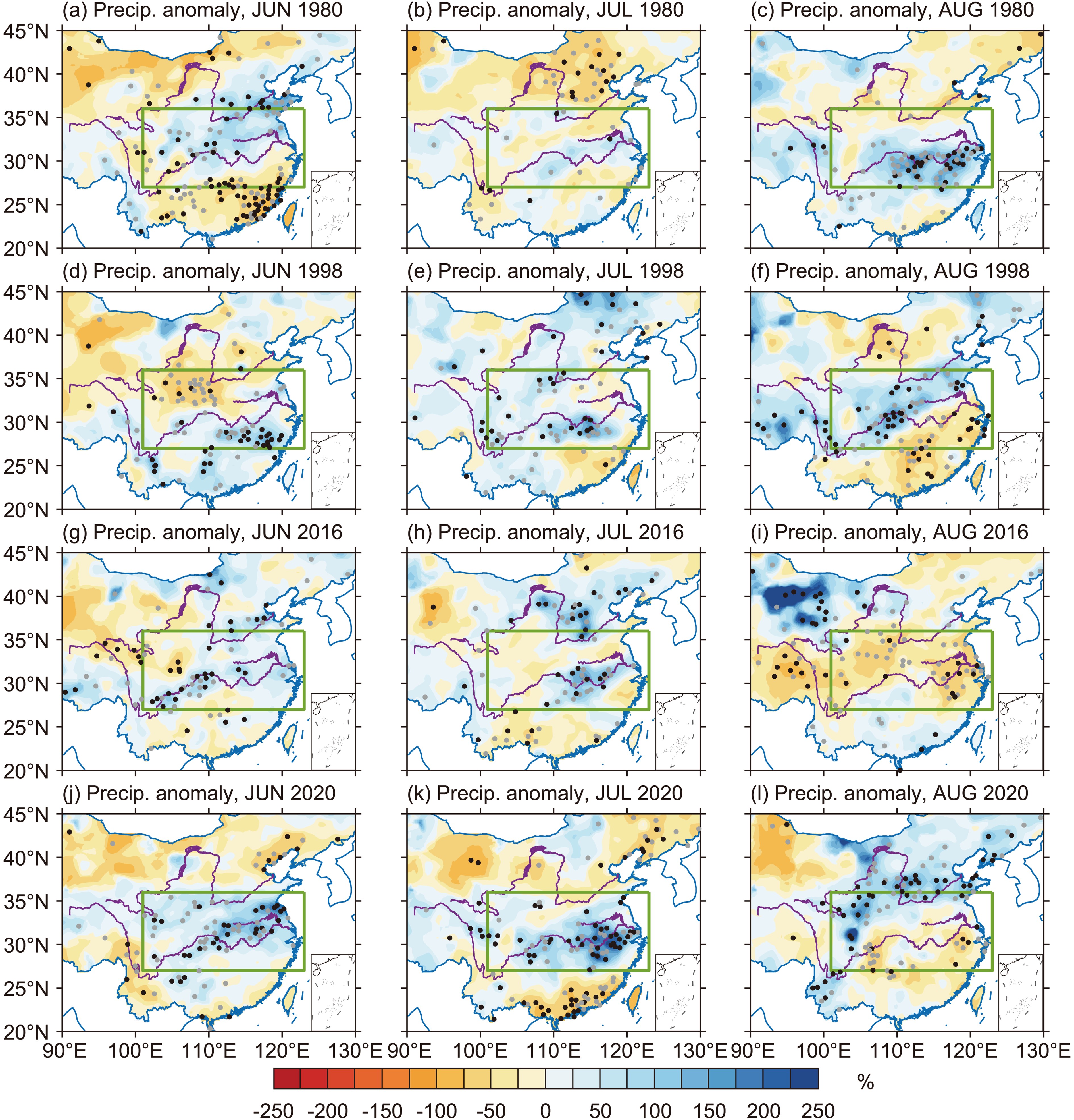

Figure2. Monthly precipitation anomaly percentages (shaded contours, units: %) during JJA (a–c) 1980, (d–f) 1998, (g–i) 2016, and (j–l) 2020, respectively, where (a, d, g, j), (b, e, h, k), (c, f, i, l) are for June, July, and August, respectively. The gray (black) dots indicate the stations where the values exceed the 95th percentile or are below the 5th percentile (are the highest or lowest) during 1979–2020. The green boxes indicate the CC region. The data are derived from station observation.

Several representative years (1980, 1998, and 2016) are selected for comparison. These years were selected because (i) Both summer 1998 and summer 2016 were characterized by heavy floods and were after a strong El Ni?o; (ii) the situations for 1980 were similar to those in 2020; the area-averaged precipitation was ranked third and only lower than that in 1998 and 2020; this year was also after a CP El Ni?o (Fig. 1c). Note that we exclude the strong EP El Ni?o event in 1983 because the summer circulation and precipitation anomalies were very similar to those in 1998 (figures not shown). We also note the exception that the total summer precipitation in 2016 was not particularly large (Fig. 1c), which is due to some special causes and will be specified in subsection 3.5. In comparison, the duration of excessive precipitation in 1980 and 2016 (Figs. 2a–c, g–i) was shorter than in 1998 (Figs. 2d–f) and 2020; the coverage and amplitude of positive precipitation anomalies in 2020 exceeded those in 1998.

2

3.2. Circulation and moisture condition anomalies

-->

3.2. Circulation and moisture condition anomalies

There was a prominent NWPAC at 850 hPa in summer 2020 (Fig. 3a). At 500 hPa, the NWP subtropical high extended anomalously westward. In addition, an anomalous low-pressure center appeared from Central Asia to Lake Baikal (Fig. 3b), indicating frequent activity of shortwave troughs in this area, which was conducive to the southward transport of cold air. The South Asian High (SAH) at 200 hPa intensified and extended eastward over the CC region, which significantly increased the westerly jet near 35°N on the north side of the SAH (Fig. 3d) and provided divergent conditions in the upper atmosphere of the CC region. The ascending anomalies in the CC region were observed throughout the entire troposphere, where the east and west centers (Fig. 3f) corresponded to the two positive precipitation anomaly centers (Fig. 1a). Most of the ascending anomalies were balanced by the descending anomalies south of the CC region in the meridional circulation (Fig. 3e).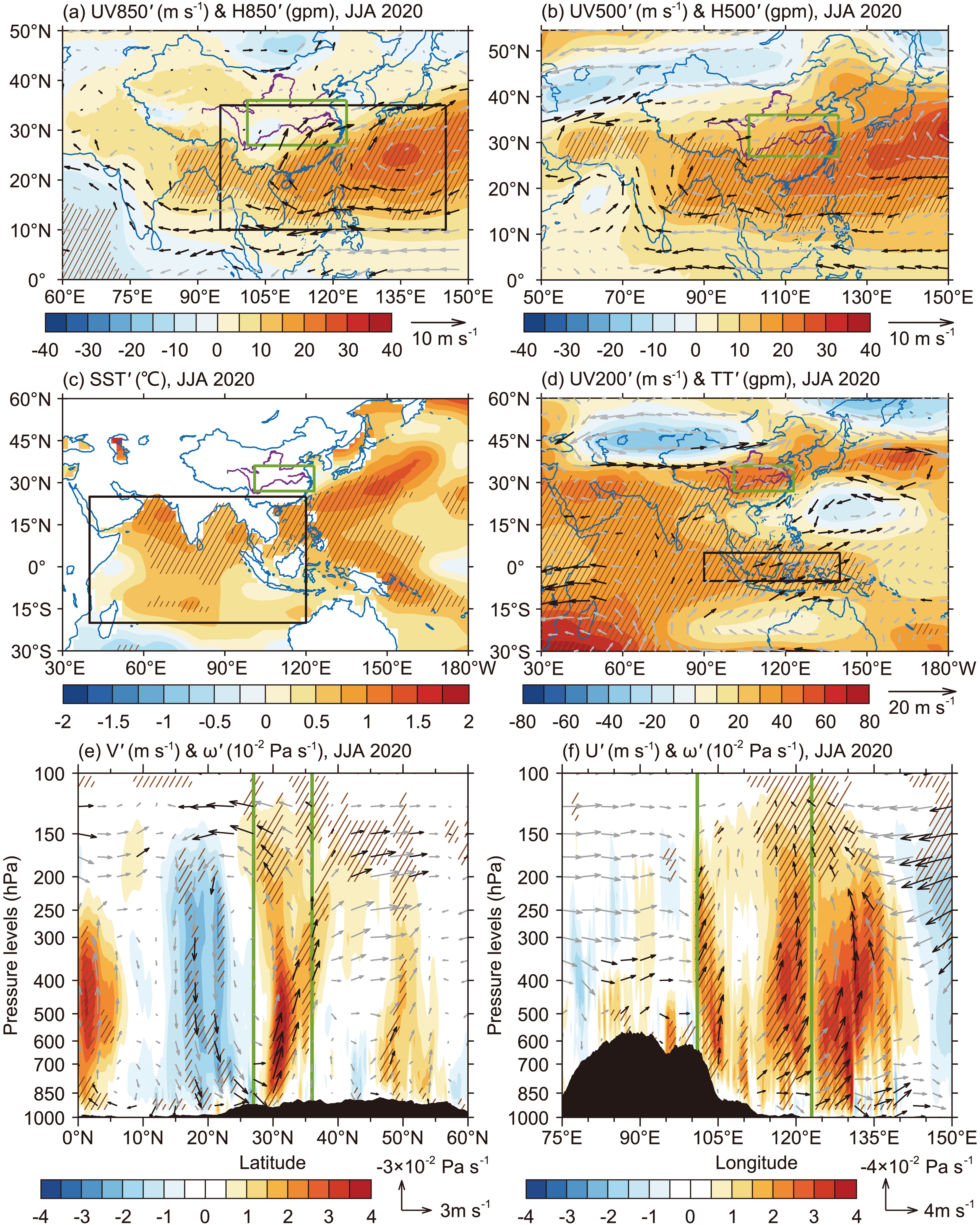

Figure3. JJA-mean wind (vectors, units: m s^?1) and geopotential height (shaded contours, units: gpm) anomalies in 2020 at (a) 850 hPa and (b) 500 hPa, respectively; (c) JJA-mean SST (shaded contours, units: °C) anomalies in 2020; (d) JJA-mean wind at 200 hPa (vectors, units: m s^?1) and TT (shaded contours, units: gpm) anomalies in 2020; (e) the vectors are composites of JJA-mean meridional wind (units: m s^?1) and vertical velocity (units: 10^?2 Pa s^?1) anomalies in 2020 at the meridional-vertical section averaged within 101°–123°E, and the shaded contours are only for vertical velocity anomalies; (f) is similar to (e) but for composites of zonal wind and vertical velocity anomalies at the zonal-vertical section averaged within 27°–36°N. The vectors in black (gray) denote that the anomalies either (neither) exceed the 95th percentile or (nor) are below the 5th percentile during 1979–2020; the hatched areas indicate where the anomalies exceed the 95th percentile or are below the 5th percentile during 1979–2020 for the shaded contours. The black box in (a), (c), and (d) indicate the NWP, TIO, and MC regions, respectively. The green boxes indicate the CC region. The SST data are from ERSSTv5, and the other variables are from ERA5.

The anomalous southwesterlies in the CC region caused by the NWPAC produced intense water vapor flux anomalies, which increased the moisture content in the entire troposphere (Fig. 4a) and generated anomalous water vapor convergence (Fig. 4b) under appropriate dynamic and thermal conditions. Moreover, the increased TT over the CC region (Fig. 3d) enhanced the saturated water vapor pressure, which could have also increased the moisture content.

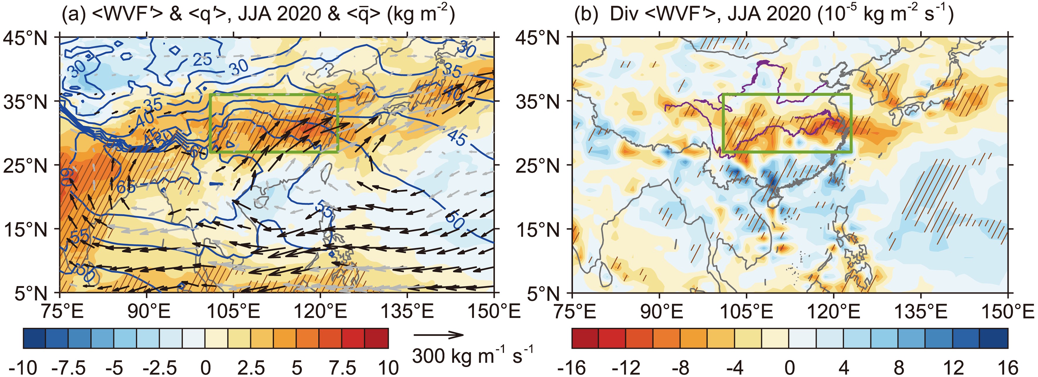Figure4. (a) JJA-mean vertical integrated water vapor flux (WVF) (vectors, units: kg m^?1 s^?1) and moisture content (that is, specific humidity) (shaded contours, units: kg m^?2) anomalies in 2020 and climatological JJA-mean summer moisture content (blue contours, units: kg m^?2) during 1979–2020; (b) JJA-mean divergence anomalies of integrated WVF (shaded contours, units: 10^?5 kg m^?2 s^?1) in 2020. The meaning of the black and gray vectors and hatched areas are the same as in Fig. 3. The green boxes indicate the CC region. The wind and specific humidity data are from ERA5.

The TIO experienced basinwide warming in summer 2020 (Fig. 3c), which generated positive TT anomalies over the TIO and excited the eastward Kelvin wave response over the MC region (Fig. 3d). Combined with the significant NWPAC (Fig. 3a), the oceanic and atmospheric responses in 2020 are consistent with the typical effect path of the IPOC following El Ni?o (Xie et al., 2009, 2016).

2

3.3. Moisture budget

-->

3.3. Moisture budget

We calculate the area-averaged values of each term in the moisture budget equation, Eq. (1), within the CC region during JJA for each year from 1979 to 2020. Considering that the 2019/20 event is an FD CP El Ni?o, we mainly analyze the relationships between the FD EMI and the moisture budget values. We use scatterplots (Fig. 5) to represent these values so that we can determine the main terms that contribute to the precipitation anomalies (P') and whether ENSO significantly affects these terms for the years of interest (1980, 1998, 2016, and 2020) in our study.

Figure5. Scatterplots between the FD EMI and the JJA-mean values of each term in the moisture equation, Eq. (1), for each year during 1979–2020, where (a–g) correspond to each term from left to right in Eq. (1) in sequence. All the values are averaged within the CC region. The thick gray lines are linear fittings of each scatter; the correlation coefficients (r) and corresponding significance levels (p) are marked at the top-left corner of each panel. The vertical and horizontal dashed lines indicate the critical values of FD CP El Ni?o/La Ni?a definitions and ±1 standard deviation values of each term, respectively. The scatters of 1979–99 (2000–19) are marked in blue (pink); the years 1980, 1998, 2016, and 2020 are marked with squares, triangles, diamonds, and pentagrams, respectively. The data to calculate the terms in Eq. (1) are from ERA5 except for the precipitation data, which is obtained from station observation.

The evaporation term (E') and advection and convection transport of anomalous water vapor by climatological airflow terms $\Big ( -\left\langle \bar{\boldsymbol{u}}\cdot {\nabla }_{h}{q}' \right\rangle $

and $ -\left\langle \bar{\omega }{\partial }_{p}{q}' \right\rangle \Big) $

(Figs. 5b, c, e) scarcely contribute to P' for all of these years. The transport of climatological water vapor by anomalous horizontal wind $\left( -\left\langle {\boldsymbol{u}}'\cdot {\nabla }_{h}\bar{q} \right\rangle \right )$

and the transport of climatological water vapor stratification by anomalous vertical motion $ \left( -\left\langle \omega '{\partial }_{p}\bar{q} \right\rangle \right) $

were the main contributors to P' in summer 2020 (Figs. 5d, f). The former is due to the southwesterly anomalies generated by the NWPAC, which transports air masses with high mean moisture to the low mean moisture area (Fig. 4a), while the occurrence of anomalous vertical motion will be further explained by the MSE budget equation. The situation in 1998 was similar to that in 2020, but for 2020 the contribution of the $ -\left\langle \omega '{\partial }_{p}\bar{q} \right\rangle $

term is greater (Fig. 5f), and the dissipation effect of the nonlinear term is smaller (Fig. 5g). However, the contributions of these terms in 2016 were negative, and the possible reasons will be discussed in subsection 3.5.
Among these terms, only P' and $ -\left\langle {\boldsymbol{u}}'\cdot {\nabla }_{h}\bar{q} \right\rangle $

are significantly (significance level p < 0.05) correlated with the FD EMI (Figs. 5a, d). We also replace the FD EMI with the D(0)JF(1) Ni?o-3 index and D(0)JF(1) EMI to make similar comparisons (figures not shown). The correlations for these two terms with the D(0)JF(1) Ni?o-3 index become more significant (p < 0.01), but the correlations for these two terms with the D(0)JF(1) EMI are weak (p > 0.1). These results confirm that in the El-Ni?o-decaying summers, EP El Ni?o exerts a more significant impact on East Asian circulations than CP El Ni?o (Feng et al., 2011; Yuan and Yang, 2012), while in the summer of an FD CP El Ni?o, a developing La Ni?a can also complement the NWPAC and thus enhance precipitation in East Asia (Feng et al., 2011; Xiang et al., 2013; Chen et al., 2016; Jiang et al., 2019). However, we observe a large departure from the fitting line between the $ -\left\langle {\boldsymbol{u}}'\cdot {\nabla }_{h}\bar{q} \right\rangle $

term and the FD EMI for the point of 2020 (Fig. 5d), which is different from the point of 1998 that is distributed near the fitting line between this term and the Ni?o-3 index (figure not shown). This situation means that the FD CP El Ni?o associated circulation anomalies are still insufficient to explain the anomalies in summer 2020.

2

3.4. MSE budget

-->

3.4. MSE budget

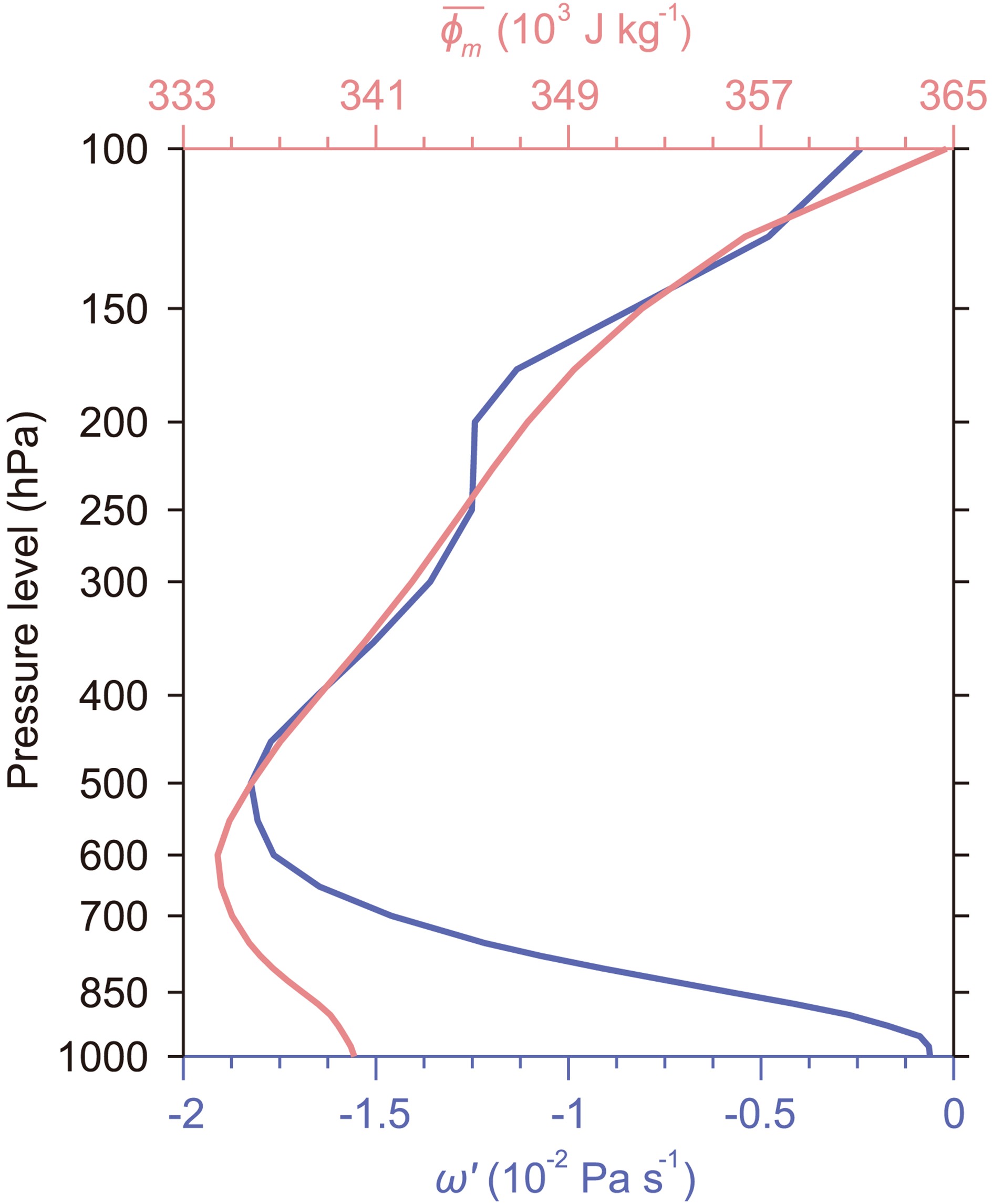The climatological JJA-mean MSE profile in the CC region is shown in Fig. 6, where the minimum value is observed at approximately 600 hPa. For summer 2020, there were ascending anomalies (ω' < 0) throughout the troposphere, with the maximum ascending anomaly observed at 500 hPa (Fig. 6). In this regime, $ \left\langle \omega '{\partial }_{p}\bar{{\phi }_{m}} \right\rangle >0 $

(Fig. 7a). Under the constraint of MSE conservation (Neelin and Held, 1987), ascending anomalies in a deep convection environment export MSE from the atmospheric column, resulting in moist convective instability (Back and Bretherton, 2009). Here, we budget each term on the right-hand side of the MSE equation, Eq. (2), to determine the critical factors for generating the anomalous vertical motions.

Figure6. Vertical profiles of vertical velocity anomalies (ω', blue line, units: 10^?2 Pa s^?1) in summer 2020 and climatological JJA-mean MSE ($ \overline{{\phi }_{m}} $

, pink line, units: J kg^?1) during 1979–2020 averaged within the CC region.

Figure7. Similar to Fig. 5 but for the FD EMI with each term in the MSE equation, Eq. (2).

For summer 2020, the effects of radiation and heat flux ($ {F}_{\mathrm{n}\mathrm{e}\mathrm{t}}' $

), advection transport of anomalous moist enthalpy by climatological horizontal winds ($ -\left\langle \bar{\boldsymbol{u}}\cdot {\nabla }_{h}{h}_{m}' \right\rangle $

), and convection transport of anomalous MSE by climatological vertical motions $ \left(-\left\langle \bar{\omega }{\partial }_{p}{\phi }_{m}' \right\rangle \right) $

are negligible (Figs. 7b, c, e); the nonlinear term has a certain negative effect (Fig. 7f); the main contribution term is the transport of climatological moist enthalpy by anomalous horizontal wind ($ -\left\langle {\boldsymbol{u}}'\cdot {\nabla }_{h}\overline{{h}_{m}} \right\rangle $

, Fig. 7d). Combined with the results in subsection 3.3, we can indicate that the anomalous southwesterlies on the northwest side of the NWPAC not only provided excess moisture but also reduced the convective stability in the CC region by transporting moist enthalpy, and thus, excited anomalous ascent. The horizontal distribution of climatologic moist enthalpy is not shown but is very similar to that of moisture content (Fig. 4a). Similar results can be obtained for 1998 and 1980.
The correlation characteristics for these terms and the Ni?o indices are similar to those presented in Fig. 5. For the right-hand side of the MSE equation, the unique term $ \Big( -\left\langle {\boldsymbol{u}}'\cdot {\nabla }_{h}\overline{{h}_{m}} \right\rangle \Big) $

that is significantly (p < 0.05) correlated with the FD EMI is also related to the NWPAC, but the value of this term in 2020 is also far from its fitting line with the FD EMI (Fig. 7d).

2

3.5. Attributions

-->

3.5. Attributions

According to the above analyses, the NWPAC is crucial not only to extreme precipitation in the CC region in summer 2020 but also in associating precipitation of this region with ENSO.
The IPOC effect path is demonstrated in Eq. (3) and Figs. 8c–f. NWPACI denotes the NWPAC index, which is defined as the area-averaged rotation of summertime wind field at 850 hPa within the NWP region (black box in Fig. 3a) multiplied by –1. This NWPACI is highly correlated with that defined by Xie et al. (2009) but has a better reflection on CC precipitation (figure not shown). The numbers in Eq. (3) represent the correlation coefficients (r) between each pair of these variables during 1979–2020; these correlations are all significant (p < 0.05). The ranges of the TIO region and MC region are shown in Figs. 3c and 3d, respectively.

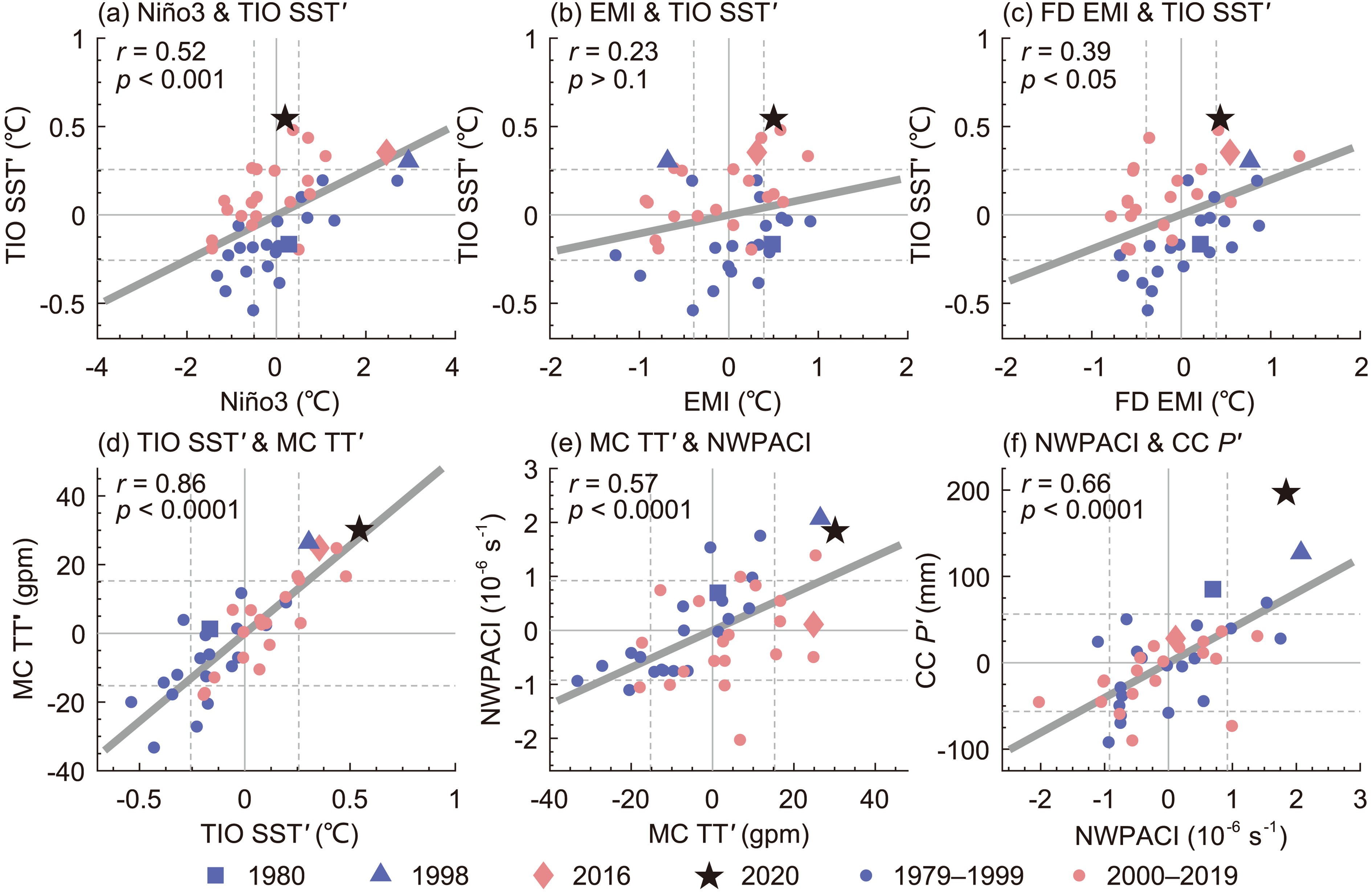Figure8. Scatterplots for the (a) D(0)JF(1) Ni?o-3 index, (b) D(0)JF(1) EMI, and (c) FD EMI with JJA-mean TIO SST anomalies, respectively. Scatterplots between JJA-mean (d) TIO SST and MC TT, (e) MC TT and NWPACI, (f) NWPACI and CC precipitation anomalies, respectively. The dashed lines indicate the critical values defining El Ni?o/La Ni?a for the Ni?o indices and ±1 standard deviation for other factors, respectively.

Scatterplots in Figs. 8a–c compare the effects of different types of El Ni?os on TIO basinwide warming. The correlation coefficient for the JJA TIO SST with the FD EMI (Fig. 8c) is significantly higher than that with the D(0)JF(1) EMI (Fig. 8b) but is lower than that with the Ni?o-3 index (Fig. 8a). When the FD Ni?o-3 index is controlled, the partial correlation between the JJA TIO SST and the FD EMI is still significant (r = 0.31, p < 0.05). These results indicate that TIO basinwide warming in response to FD CP El Ni?o is stronger than that to general CP El Ni?o, which is also demonstrated in other studies based on different classifications (Chowdary et al., 2017; Jiang et al., 2019). The causes of the stronger TIO basinwide warming involve air–sea coupling processes (Chowdary et al., 2017; Jiang et al., 2017); we will not go into detail here. It is also found that the correlation between the FD EMI and the NWPACI (r = 0.55, p < 0.001) enhances significantly compared with that between the D(0)JF(1) EMI and the NWPACI (r = 0.18, p > 0.1; figures not shown). Several processes may be responsible for this enhancement in addition to the contribution of the stronger TIO basinwide warming. During FD El Ni?o summers, the ascending branch of the Walker circulation returns to the MC region, which increases the Kelvin wave response over this region; the establishment of the negative TCEP SST anomalies stimulate the atmospheric Rossby wave response over the NWP; these processes also supplement the NWPAC (Jiang et al., 2019). Therefore, distinguishing FD CP El Ni?os from general CP El Ni?os can better explain the circulation and precipitation anomalies in summer 2020.
The point of 2020 is still an outlier far above the fitting line with respect to the FD EMI (Fig. 8c), which is unlike the points of 1998 and 2016 that are distributed near the fitting line relative to the Ni?o-3 index (Fig. 8a). Note that in Figs. 8a–c, most of the points during 1979–99 (2000–20) are distributed below (above) the fitting line. This is because the TIO SST presents a significant (p < 0.01 for a Mann-Kendall test) increasing trend during these decades (Fig. 9a), which is independent of the decadal ENSO variations (Fig. 1c). A similar trend is observed for the MC TT (Fig. 9a). Although the NWPACI does not have an increasing trend as do the TIO SST and MC TT, most of the high NWPACI cases match the high values of TIO SST or MC TT, such as for the years 1983, 1986, 1998, 2010, and 2020 (green dots in Fig. 9a). Therefore, we infer that the TIO warming trend in recent decades may provide a favorable background to generate an extremely strong NWPAC during El-Ni?o-decaying summers; the extreme precipitation in summer 2020 was a manifestation under suitable conditions. Nevertheless, some cases are exceptions. For example, in summer 2015/16, both the positive TIO SST and MC TT anomalies were very strong, but the NWPAC was very weak (Figs. 8c–e). The weak NWPAC hindered moisture and moist enthalpy transport (Figs. 5d and 7d); thus, the positive precipitation anomaly in summer 2016 was not so pronounced (Fig. 1c). The negative rainfall anomalies in the CC region in August 2016 (Fig. 2i) imply that the circulation conditions were not able to sustain the NWPAC until late summer. Some studies suggested the intra-seasonal evolution of the TIO SST (Wang et al., 2017) and the effect of southeast TIO warming (Chen et al., 2018) to explain this exception. Moreover, the factors unrelated to the IPOC, such as the PDO and ENSO variance, also modulate the NWPAC variations on the decadal timescale (Chowdary et al., 2012; Feng et al., 2014), which may explain the absent decadal trend of the NWPACI. However, it is controversial whether the TIO decadal warming trend is generated by natural variability or anthropogenic forcing (Alory et al., 2007; Du and Xie, 2008; Zheng et al., 2011; Tao et al., 2015).

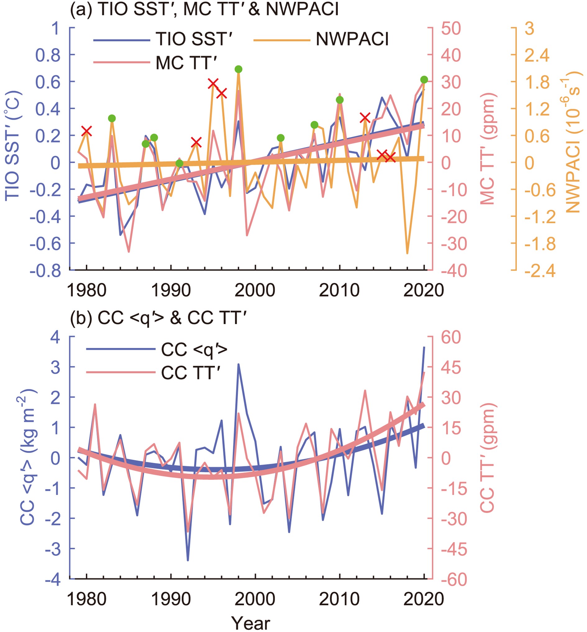Figure9. (a) Time series of the JJA-mean TIO SST anomalies (blue line, units: °C), MC TT anomalies (pink line, units: gpm), and NWPACI (yellow line, units: 10^?6 s^?1) during 1979–2020. The thick lines are linear fittings, respectively. The green points and red crosses indicate the years that positive NWPACI matches (1983, 1987, 1988, 1991, 1998, 2003, 2007, 2010, 2020) and mismatches (1980, 1993, 1995, 1996, 2013, 2015, 2016) positive TIO SST and MC TT anomalies, respectively. (b) Time series of JJA-mean vertically-integrated moisture content (blue line, units: kg m^?2) and TT (pink line, units: gpm) anomalies in the CC region; the thick lines are quadratic fittings.

The point of 2020 is still much higher than the regression line between CC precipitation and the NWPACI (Fig. 8f); some factors in addition to the NWPAC are involved. Here, we propose a possible cause. Compared with 1998, there is higher TT and moisture content over the CC region in summer 2020 (Fig. 9b). The promoted thermodynamic and moisture conditions may explain why more precipitation can be produced in 2020 (Fig. 8f). Note the increasing trends of TT and moisture content in the CC region after 2000 (Fig. 9b). However, the reason for these trends is still unknown but may be due to atmospheric responses under climate warming or due to the SAH interdecadal changes (Zhang et al., 2000).

2

3.6. Verification by numerical experiments

-->

3.6. Verification by numerical experiments

The results of 20_ALL minus CLIM reproduce the M–G pattern over the TIO (Fig. 10c), the NWPAC (albeit a more northern location compared with the actuality, Figs. 10b and 3a), and the positive precipitation anomalies (Fig. 10b) at the northwest flank of the NWPAC, which confirms that the extreme rainfall is due to the tropical SST anomalies.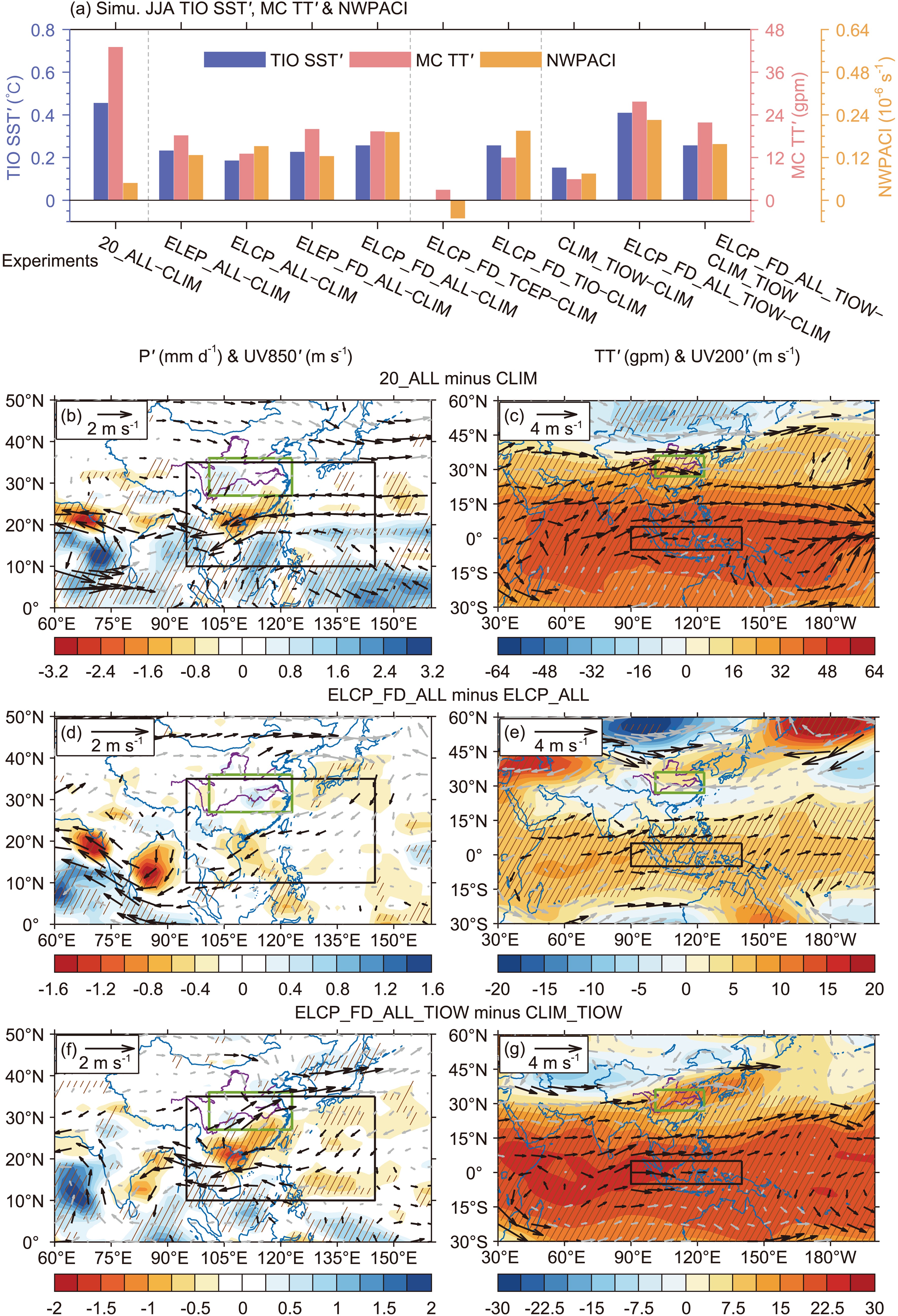

Figure10. (a) Bars of the boundary condition JJA-mean TIO SST (blue bars, units: °C) and simulated JJA-mean MC TT (pink bars, units: gpm) and NWPACI (yellow bars, units: 10^?6 s^?1) for each sensitivity experiment minus CLIM; one special case is for ELCP_FD_ALL_TIOW minus CLIM_TIOW (the last group of bars). (b) JJA-mean wind (vectors, units: m s^?1) and precipitation (shaded contours, units: mm d^?1) at 850 hPa, (c) wind (vectors, units: m s^?1) at 200 hPa and TT (shaded contours, units: gpm) for the results of 20_ALL minus CLIM. (d, e) and (f, g) are similar to (b, c) but for ELCP_FD_ALL minus ELCP_ALL and ELCP_FD_ALL_TIOW minus CLIM_TIOW, respectively. The vectors in black (gray) denote wind differences above (below) the 95% confidence level based on Student’s t-test; the hatched areas indicate the differences above the 95% confidence level based on Student’s t-test for the shaded contours. The black boxes in (b, d, f) and (c, e, g) indicate the NWP and MC regions, respectively. The green boxes indicate the CC region.

The first set of experiments demonstrates that the summertime NWPAC after an FD CP El Ni?o is stronger than that after a general CP El Ni?o, and the difference is greater than those between FD and general EP El Ni?os. According to our simulation, compared with the general CP El Ni?o, the tropospheric Kelvin wave response excited by TIO warming after the FD CP El Ni?o extends farther east, and the NWPAC is prone to have a northeast position (Figs. 10d, e), which is consistent with a previous study (Jiang et al., 2019).
The results of experiment ELCP_FD_TIO indicate that the FD CP El Ni?o associated TIO SST anomalies can individually force a significant NWPAC. However, when only the TCEP SST anomalies are considered, the simulated NWPACI is slightly negative according to our results from ELCP_FD_TCEP (Fig. 10a), which is somewhat different from previous research (Chen et al., 2016; Jiang et al., 2019). It can be inferred that the rapid cooling of the TCEP during the FD CP El Ni?o may not contribute to the summertime NWPAC, and the local air–sea interaction needs to be considered (Wu et al., 2010).
Comparing the NWPACI derived from ELCP_FD_ALL_TIOW minus CLIM with ELCP_FD_ALL minus CLIM (Fig. 10a), model results verify that a stronger summertime NWPAC can be excited after an FD CP El Ni?o under the background of the decadal TIO warming. However, according to our simulation, the intensified NWPAC is due to the NWPAC being produced by decadal TIO warming unrelated to ENSO (CLIM_TIOW minus CLIM in Fig. 10a) rather than the intensified IPOC effect when the TIO is in a warmer state (ELCP_FD_ALL_TIOW minus CLIM_TIOW in Fig. 10a), which is different from the observation that the NWPAC has no decadal strengthening trend (Fig. 9a). We performed a supplemental experiment similar to CLIM_TIOW, but the TIO decadal SST differences were replaced by those of the tropical Pacific. The results manifest a negative effect of the tropical Pacific SSTs on the decadal NWPAC variation (figure not shown), so the positive effect from the TIO could be offset. The summertime circulation anomaly patterns for ELCP_FD_ALL_TIOW minus CLIM_TIOW (Figs. 10f, g) are similar to those in 2020 (Figs. 3a, d). Compared with the patterns illustrated in Figs. 10c–d, the tropospheric M–G pattern is mainly limited to the TIO and MC regions (Fig. 10g), and the NWPAC is located relatively southwest, which is more conducive to moisture convergence in the CC region (Fig. 10f).

4. Conclusions and discussion

This study investigates the causes of the record-breaking precipitation that happened in the CC region during summer 2020 from the perspective of ENSO-induced oceanic and atmospheric responses. In summer 2020, the weak CP El Ni?o event of 2019/20 rapidly decayed as a La Ni?a developed. Via the IPOC effect path, an extremely strong anomalous anticyclone appeared over the NWP. The anomalous southwesterlies on the northwest side of the NWPAC contributed excess water vapor required for precipitation and transported moist enthalpy to reduce the convective stability in the CC region, triggering ascending anomalies and thus producing extreme precipitation. However, the weak CP ENSO activity was not sufficient enough on its own to explain such extremely strong NWPAC and precipitation. We inferred three possible mechanisms to resolve this dilemma, and the first two mechanisms were verified using the numerical model. (i) Most importantly, the TIO warming trend in recent decades may cause an extremely strong NWPAC to be generated in the summer after an El Ni?o, even if it is a weak El Ni?o. (ii) The FD CP El Ni?o is distinct from the general CP El Ni?o in affecting the Asia-Pacific region climate and circulations; the former can produce a stronger TIO warming, M–G pattern response over the TIO, and NWPAC. (iii) The increasing trend of TT and atmospheric moisture content in the CC region after 2000 may produce more precipitation even if the NWPAC intensity does not change.
Some evidence from previous studies also supports our first inference. The warmer TIO in recent decades increases the correlation between ENSO and the EASM by enhancing the impact of ENSO on the NWPAC (Huang et al., 2010; Xie et al., 2010). As the global climate warms, the TIO warming trend will persist, and the IPOC effect will be strengthened (Zheng et al., 2011; Chu et al., 2014). However, these studies did not involve the problem of the extreme NWPAC occurrences. Coupled Model Intercomparison Project Phase 5 or Phase 6 (CMIP5/6) data will be analyzed to verify our inference further.
Although we have discussed the possible reasons for the exceptions of the mismatched NWPAC in subsection 3.5, some cases are still elusive. It is interesting that in the summers of 1980, 1993, 1995, and 1996, a relatively strong NWPAC appeared without corresponding strong TIO basinwide warming and increase in MC TT (Fig. 9a). The summer precipitation anomalies in the CC region in these years are also positive (Fig. 1c). We generally consider the increased EASM precipitation to be a result of the NWPAC (Zhang et al., 2017), and the NWPAC maintenance is attributed to the forces from the tropical ocean and atmosphere (Wang et al., 2000; Xie et al., 2009; Wu et al., 2010, 2017; Xiang et al., 2013; Chen et al., 2016; Jiang et al., 2019). However, whether the extratropical convective activity anomalies can, in turn, drive the NWPAC is an issue worth investigating.
We define the FD Ni?o indices and screen FD ENSO events with only simple criteria in this study. With our definition, some strong EP El Ni?o cases, such as 1998 and 2016, are also observed as high values of the FD EMI (Figs. 1c and 8c); this is because CP La Ni?a events developed in these years. Nevertheless, our outcomes agree with previous studies regarding the decay pace of El Ni?o (Chen et al., 2016; Chowdary et al., 2017; Jiang et al., 2019). In future investigations, it will be necessary to construct an optimal FD ENSO definition that satisfies the self-explanation of mechanisms and meets the requirement of improving prediction. Of course, it is difficult to derive relatively universal laws from short-duration observation data, which greatly limits our understanding of record-breaking events; accurate paleoclimate data can be an outlet to break these limitations.
Acknowledgements. This study was jointly supported by grants from the Strategic Priority Research Program of the Chinese Academy of Sciences (CAS) (Grant No. XDB40000000), the CAS (Grant No. QYZDJ–SSW–DQC021), the National Natural Science Foundation of China (Grant No. 41630531), and the State Key Laboratory of Loess and Quaternary Geology. We thank the supercomputer center of the Pilot Qingdao National Laboratory for Marine Science and Technology and Beijing Super Cloud Computing Center, who offered computing services. We also thank Dr. X. Z. LI, H. LIU, and L. LIU from the Institute of Earth Environment, CAS, who offered suggestions for our numerical experiments.

本站小编 Free考研考试/2022-01-02

Corresponding author: Yu LIU,yuliu2018@ieecas.cn;

HTML

2.1. Data

2.2. Methods

2.3. Model

3.1. Precipitation anomalies in summer 2020 and comparisons with other cases

3.2. Circulation and moisture condition anomalies

3.3. Moisture budget

3.4. MSE budget

3.5. Attributions

3.6. Verification by numerical experiments

相关话题/Extreme Rainfall Occur

领限时大额优惠券,享本站正版考研考试资料!

The Extraordinary Rainfall over the Eastern Periphery of the Tibetan Plateau in August 2020

Atmospheric Rivers and Mei-yu Rainfall in China: A Case Study of Summer 2020

Typical Circulation Patterns and Associated Mechanisms for Persistent Heavy Rainfall Events over Yan

Two Types of Diurnal Variations in Heavy Rainfall during July over Korea

On the Diurnal Cycle of Heavy Rainfall over the Sichuan Basin during 10–18 August 2020

Seasonal Rainfall Forecasts for the Yangtze River Basin in the Extreme Summer of 2020

Decadal Change in the Influence of the Western North Pacific Subtropical High on Summer Rainfall ove

PV Perspective of Impacts on Downstream Extreme Rainfall Event of a Tibetan Plateau Vortex Collabora

Impacts of Irrigation and Vegetation Growth on Summer Rainfall in the Taklimakan Desert

Changes of Extreme Precipitation and its Associated Mechanisms in Northwest China