Fund Project:Project supported by the National Natural Science Foundation of China (Grant Nos. 11835011, 12004338)
Received Date:05 February 2021
Accepted Date:15 April 2021
Available Online:07 June 2021
Published Online:20 September 2021
Abstract:The characteristics of fundamental and mutipole dark solitons in the nonlocal nonlinear couplers are studied through numerical simulation in this work. Firstly, the fundamental dark solitons with different parameters are obtained by the Newton iteration. It is found that the amplitude and beam width of the ground state dark soliton increase with the enhancement of the nonlocality degree. As the nonlinear parameters increase or the propagation constant decreases, the amplitude of the fundamental dark soliton increases and the beam width decreases. The power of the fundamental dark soliton increases with the nonlocality degree and nonlinear parameters increasing, and decreases with the propagation constant increasing. The refractive index induced by the light field decreases with the nonlocality degree increasing and the propagation constant decreasing. The amplitudes of the two components of the fundamental dark soliton can be identical by adjusting the coupling coefficient. These numerical results are also verified in the case of multipole dark solitons. Secondly, the transmission stability of fundamental and mutipole dark solitons are studied. The stability of dark soliton is verified by the linear stability analysis and fractional Fourier evolution. It is found that the fundamental dark solitons are stable in their existing regions, while the stable region of the multipolar dark solitons depends on the nonlocality degree and the propagation constant. Finally, these different types of dark dipole solitons and dark tripole solitons are obtained by changing different parameters, and their structures affect the stability of dark soliton. It is found that the multipole dark soliton with potential well is more stable than that with potential barrier. The refractive-index distribution dependent spacing between the adjacent multipole dark solitons favors their stability. Keywords:nonlocal nonlinearity/ dark soliton/ stability
假设方程(3)和方程(4)的初解形式为 $W_{j} = $$ A_{j} \tanh(x)$, $ M_{j} = B_{j}\exp(-x^2) $, 其中$ A_{j} $ ($ j $ = 1, 2)是复合光场的振幅; $ B_{j} $ ($ j $ = 1, 2)是诱导折射率的振幅; 选择合适的参数$ \alpha_{1} $ = 1, $ \alpha_{2} $ = 2, $ \beta_{1} $ = –2, $ \beta_{2} $ = –1, $ A_{1} $ = 1, $ A_{2} $ = 2, $ B_{1} $ = 1, $ B_{2} $ = 1和$ d \leqslant 12 $的非负数, 把$ W_{j} $和$ M_{j} $的初值代入方程(3)和方程(4)中作为初始迭代解, 采用牛顿迭代的方法对方程(3)和方程(4)进行求解可以得到基态暗孤子(见图1). 图1(a)表明在其他参数不变的情况下, 非局域程度$ d $ = 2.0, 4.5, 7.5时, 不同形状的暗孤子在非局域程度$ d $增大时, 暗孤子的两个凸出的驼峰也相应增大, 而折射率随之减小且$ m_{1} $和$ m_{2} $相等. 暗孤子的幅值和束宽随非局域程度的增大而增大. 随着非局域程度的增大, 介质的非线性效应减弱, 光束的衍射效应增强, 导致孤子的宽度增大. 当非局域程度$ d $分别为$ 2.0 $, $ 4.5 $, $ 7.5 $时, 相应的功率$ P $与传播常数$ b $的关系如图1(b)所示. 可以看出, $ b $取不同的负值时, 基态暗孤子功率随$ b $的增大而减小. 当$ b $固定时, 非局域性程度$ d $越大, 功率越大, 在这样的区间内, 基态暗孤子都是存在的. 在图1(c)中, $ d $ = 2和其他参数不变的情况下, 非线性参数$ \beta_{1} $ = –2, –5, –7时, 随着非线性参数$ \beta_{1} $减小, 基态暗孤子的束宽增大, 幅值减小, 即增强非线性效应可以提高光束的振幅. 而相应的折射率$ m_{j} $的分布因非线性参数$ \beta_{j} $的变化存在一定的差异. 当$ \beta_{2} $固定时, $ m_{1} $随着$ \beta_{1} $的减少而减少, 而$ m_{2} $ 随着$ \beta_{1} $的减少而增大. 类似地, 当$ \beta_{1} $固定时, $ m_{1} $随着$ \beta_{2} $的减少而增大, 而$ m_{2} $则随着$ \beta_{2} $的减少而减少. 从图1(d)可以看出, 随着传输常数$ b $的减小, 光束宽度减小, 幅值增大, 相应的折射率减小并且$ m_{1} $和$ m_{2} $相等. 为了研究耦合系数$ \alpha_{j} $对孤子的影响, 引入耦合系数之比$ G = {\alpha_{1}}/{\alpha_{2}} $. 当$ G < 1 $时, 基态暗孤子$ U_{2} $的振幅包络随$ G $的增大而迅速减小, 并大于基态暗孤子$ U_{1} $的振幅包络. 基态暗孤子$ U_{1} $的振幅包络缓慢减小, 直到$ G $ = 1. 当$ G $ = 3.125时, 两分量基态暗孤子的振幅相等. 当$ G > 1 $时, 基态暗孤子$ U_{2} $的振幅包络变化趋于平缓, 而孤子$ U_{1} $的振幅包络随$ G $的增大而增大(见图1(e)). 可以推断, 耦合系数越大, 对自身暗孤子的幅值的影响越大, 而对耦合孤子振幅的影响相对较小. 图 1 基态暗孤子数值解 (a)不同d对应的波形($ d $分别取2.0 (蓝线), 4.5 (红线)和7.5 (绿线)); (b)功率与传播常数的关系图; (c) $ b = -1 $, $ d = 2 $, $ \beta_{2} = -1 $时, 不同$ \beta_{1} $对应的波形($ \beta_{1} $分别取–2 (蓝线), –5 (红线)和–7 (绿线)); (d) $ d $ = 2时, 不同$ b $对应的波形($ b $分别取–0.2 (蓝线), –0.5 (红线)和–1.0 (绿线)); (e)不同耦合系数比值下, $ U_{1} $和$ U_{2} $的幅值图 Figure1. Numerical solution of the ground state dark soliton: (a) Waveform corresponds to different $ d $ ($ d $ selected as 2.0 (blue lines), 4.5 (red lines) and 7.5 (green lines), respectively); (b) the power versus the propagation constant; (c) waveform corresponds to different $ \beta_{1} $ when $ b $ = –1, $ d $ = 2, $\beta_{2} = -1$ ($ \beta_{1} $ selected as –2 (blue lines), –5 (red lines) and –7 (green lines), respectively); (d) waveform corresponds to different $ b $ ($ b $ selected as –0.2 (blue lines), –0.5 (red lines) and –1.0 (green lines), respectively); (e) amplitude diagram of $ U_{1} $ and $ U_{2} $ for different coupling coefficient ratios.
23.2.基态暗孤子的线性稳定性分析 -->
3.2.基态暗孤子的线性稳定性分析
为了进一步探究基态暗孤子的动力学行为, 对基态暗孤子的传输进行稳定性分析. 最简单的方法是在初值的基础上加随机白噪声, 并用分步傅里叶方法进行数值演化. 改变传播常数和非局域程度得到的基态暗孤子可以稳定地进行长距离传播, 如图2(a)所示. 此外, 进一步证实基态暗孤子的稳定性是对其解做线性稳定性分析. 为此引入方程(1)和方程(2)的基态暗孤子的扰动解: 图 2 基态暗孤子的传输特征及稳定性 (a)$ d $ = 2, $ b $ = –1时, $ U_{1} $的加噪传输图; (b)稳定性图谱 Figure2. Propagation characteristics and stability of the ground state dark soliton: (a) Propagation of $ U_{1} $ with the white noise when $ d $ = 2 and $ b $ = –1; (b) stability profile
通过改变试探解和选择合适的参数, 可以得到偶极、三极、四极以及五极的暗孤子. 根据数值研究结果, 发现基态暗孤子中非局域程度$ d $、传播常数$ b $、非线性参数$ \beta_{j} $与暗孤子的宽度、幅值、功率之间的关系在多极暗孤子中也存在相似的关系. 多极暗孤子可以被视为多个反对称的相位分布的基态暗孤子的非线性组合(束缚态), 它们之间的作用力将它们聚集在一起. 这种束缚态不可能存在于局域克尔介质中, 因为孤子间的$ \pi $相位差会导致折射率分布在交界处有个局部下降, 并导致排斥; 相反, 在非局域克尔介质中, 由于介质具有卷积形式的非线性响应, 折射率变化取决于整个横截面上的光强分布, 因此在两个反相位孤子之间形成足够高的折射率分布, 引起两孤子的相互吸引, 当排斥相互作用最终被吸引相互作用平衡, 这样就会形成束缚态. 当$ \alpha_{1} $ = 1, $ \alpha_{2} $ = 2, $ \beta_{1} $ = –4, $ \beta_{2} $ = –2 时, 可以得到偶极暗孤子. 图3给出了偶极暗孤子的特征和传输稳定性. 偶极暗孤子折射率呈钟形分布, 顶部中心区域有1个非零倾角, 倾角两边是两个微微凸起的驼峰, 驼峰提供吸引相互作用与孤子间原有的排斥相互作用相抗衡, 这在偶极暗孤子调制稳定性中起了重要的作用, 如图3(a)所示. 类似的三极、四极以及五极也可以得到相似的暗孤子分布和折射率呈钟形分布, 只是折射率中心区域的顶部微微凸起的驼峰数与暗孤子的极数相同. 暗孤子幅值为零处, 对应的折射率出现驼峰, 此处折射率更大, 提供更大的吸引力. 图3(b)显示偶极暗孤子是区域不稳定的. 显然, 在$ -2\leqslant b \leqslant -0.2 $ 范围内, 当非局域程度$ d $增大时, 白色稳定区域变宽且移向更大的$ b $. 当传播常数$ b $固定时, 在$ 3.5\leqslant d \leqslant 6.4 $区间, 白色稳定区域向较大的$ d $移动, 进一步证实了非局域性可以调节孤子的稳定性. 在$ b $ = –1.5, $ d $ = 4.2的情况下, 在初解的基础上加白噪声作为初始扰动解, 得到偶极暗孤子传播路径不变的结果(见图3(c)). 然而, 当$ b $ = –2, $ d $ = 1.5时, 偶极暗孤子在传播过程中不能保持稳定, 如图3(d)所示. 相应的传输图(图3(c)和图3(d))证实了图3(b)中所示的稳定性分析结果是正确的. 同样地, 可以得到三极和四极甚至五极暗孤子类似的结果. 研究表明, 在非局域非线性耦合器中, 偶数极暗孤子比奇数极暗孤子更容易稳定, 并且随着极数的增加, 多极暗孤子稳定区域变窄. 图 3 偶极暗孤子的特性 (a) $ d $ = 1, $ b $ = –1时偶极暗孤子的强度分布图; (b) 线性稳定性区域图; (c) $ d $ = 4.2, $ b $ = –1.5时, $ U_{1} $传输图; (d) $ d $ = 1.5, $ b $ = –2时, $ U_{1} $传输图 Figure3. Characteristics of the dipole dark soliton: (a) Intensity profiles of dipole dark soliton when $ d $ = 1 and $ b $ = –1; (b) linear stability region diagram; (c) transmission diagram of $ U_{1} $ when $ d $ = 4.2 and $ b $ = –1.5; (d) transmission diagram of $ U_{1} $ when $ d $ = 1.5 and $ b $ = –2
24.2.不同类型的偶极暗孤子及其稳定性 -->
4.2.不同类型的偶极暗孤子及其稳定性
在这一节中, 分析不同类型的偶极暗孤子的传输特性, 数值结果如图4所示. 当$ \alpha_{1} $ = 1, $ \alpha_{2} $ = 2, $ \beta_{1} $ = –2, $ \beta_{2} $ = –1时, 得到图4(a)和图4(d)两种不同类型的偶极暗孤子. 图4(a)和图4(d)显示折射率在中心区域的分布几乎呈亮孤子型. 折射率达到最大值时, 暗孤子的幅值为零, 此处吸引相互作用最大. 在图4(a)中的两个暗孤子形成1个势阱, 对应的折射率分布区域形成1个波谷, 波谷的宽度决定孤子的间距, 即孤子间距越大, 波谷的宽度就越宽. 图4(a)中两暗孤子间距为$ 10 $, 在初值的基础上加白噪声作为初始微扰解进行传播时, 发现两暗孤子能以蛇形稳定传输(见图4(b)). 为了更好地证明其传输稳定性, 图4(c)给出了线性扰动增长率$ \lambda $的实部和虚部, $ \lambda $的实部为零, 这验证了图4(b)的传输演化结果. 相反地, 在图4(d)中, 在偶极暗孤子之间形成势垒, 这导致吸引相互作用和排斥相互作用之间存在竞争. 在中心轴上, 偶极暗孤子相距最近, 对应的折射率最小, 相互排斥作用最大. 随着折射率的增大, 吸引相互作用增大, 直到两个孤子相距最远. 在这种情况下, 偶极暗孤子沿z方向周期性传输, 如图4(e)所示. 经过线性稳定性分析, 发现其扰动增长率$ \lambda $存在实部. 值得注意的是, 耦合器中还存在高度对称的两个偶极暗孤子. 当$ \alpha_{1} $ = 1, $ \alpha_{2} $ = 2, $ \beta_ {1} $ = –4, $ \beta_{2} $ = –2时, 可以得到图4(g)和图4(i)所示的两个偶极暗孤子. 在图4(g)中, 在两个偶极孤子之间形成1个势阱, 相邻两个偶极孤子之间的孤子间距为$ 8 $. 显然, 两个偶极暗孤子的传输互不干扰, 传输过程中的整个波形可以保持稳定, 如图4(g)所示; 相反, 在图4(i)中, 两个偶极暗孤子之间形成势垒, 相邻两个偶极暗孤子之间的距离为$ 5 $, 比图4(g)中的距离窄. 在这种情况下, 两个偶极暗孤子传输很短的距离就开始扩散(见图4(j)), 其传输机制与图4(e)的偶极暗孤子类似. 从以上结果可以得知: 分开的偶极暗孤子之间存在周期性相互作用, 为了减弱这种孤子间的干扰, 一种方法是使孤子间距足够大, 使折射率中心区域的波谷宽度达到吸引相互作用等于排斥相互作用时的宽度. 很明显, 图4(d)中的孤子间距小于图4(a), 图4(g)的孤子间距大于图4(i), 图4(d)和图4(i)中的暗孤子在短距离内周期性传输就开始振动(见图4(e)和图4(j)), 可以得出孤子间距对偶极暗孤子的稳定性有影响. 图 4 不同类型的偶极暗孤子的强度分布和传播特性 (a)?(c)分别为$ d $ = 4, $ b $ = –1.5时, 偶极暗孤子的强度分布图、传输图和稳定性图谱; (d)?(f) 分别为$ b $ = –1.3, $ d $ = 1时, 偶极暗孤子的强度分布图、传输图和稳定性图谱; (g)和(h)分别为$ b $ = –1.7, $ d $ = 2时, 两个偶极暗孤子的强度分布和$ U_{1} $的传输图; (i) 和(j)分别为$ b $ = –1.4, $ d $ = 5时, 两个偶极暗孤子的强度分布和$ U_{1} $的传输图 Figure4. Intensity profiles and propagating characteristics of different types of dipole dark soliton: (a)– (c) The intensity distribution diagram, the transmission diagram and the stability diagram of the dipole dark soliton when $ d $ = 4 and $ b $ = –1.5 respectively; (d)?(f) the intensity distribution diagram, the transmission diagram and the stability diagram of the dipole dark soliton when $ b $ = –1.3 and $ d $ = 1 respectively; (g) and (h) the intensity distribution of dipole-dipole dark solitons and the transmission diagram of $ U_{1} $ when $ b $ = –1.7 and $ d $ = 2, respectively; (i) and (j) the intensity distribution of dipole-dipole dark solitons and the transmission diagram of $ U_{1} $ when $ b $ = –1.4 and $ d $ = 5, respectively.
24.3.三极暗孤子及其稳定性 -->
4.3.三极暗孤子及其稳定性
当$ \alpha_{1} $ = 1, $ \alpha_{2} $ = 2, $ \beta_{1} $ = –2, $ \beta_{2} $ = –1时, 可以得到三极暗孤子. 从图5(a)和图5(c)可以看出, 传输稳定性的性质与偶极暗孤子相似. 在相邻的两个孤子之间形成势阱, 使得暗孤子更容易稳定传输; 相反, 两个相邻的孤子之间形成势垒, 孤子传输很短一段距离就开始发散, 很难保持稳定. 比较图5(a)和图5(c), 图5(c)中的三极暗孤子之间形成势垒, 对应的折射率分布区域形成波谷, 波谷的宽度对应了孤子间的间距. 图5(c)中的孤子间距为4.6, 比图5(a)中的孤子间距小, 图5(a)中的孤子可以长距离稳定传输. 对三极暗孤子的稳定性分析, 进一步证实了暗孤子的稳定性受孤子间距的影响. 图 5 不同类型的三极暗孤子的强度分布和传播特性 (a)和(b)分别为$ b $ = –4.45, $ d $ = 1时, 三极暗孤子的强度分布和$ U_{1} $传输图; (c)和(d)分别为$ b $ = –1.2, $ d $ = 1时, 三极暗孤子的强度分布和$ U_{1} $传输图 Figure5. Intensity profiles and propagating characteristics of tripole dark soliton: (a) and (b) The intensity distribution of the tripole dark soliton and the transmission diagram of $ U_{1} $ when $ b $ = –4.45 and $ d $ = 1, respectively; (c) and (d) the intensity distribution of the tripole dark soliton and the transmission diagram of $ U_{1} $ when $ b $ = –1.2 and $ d $ = 1, respectively.


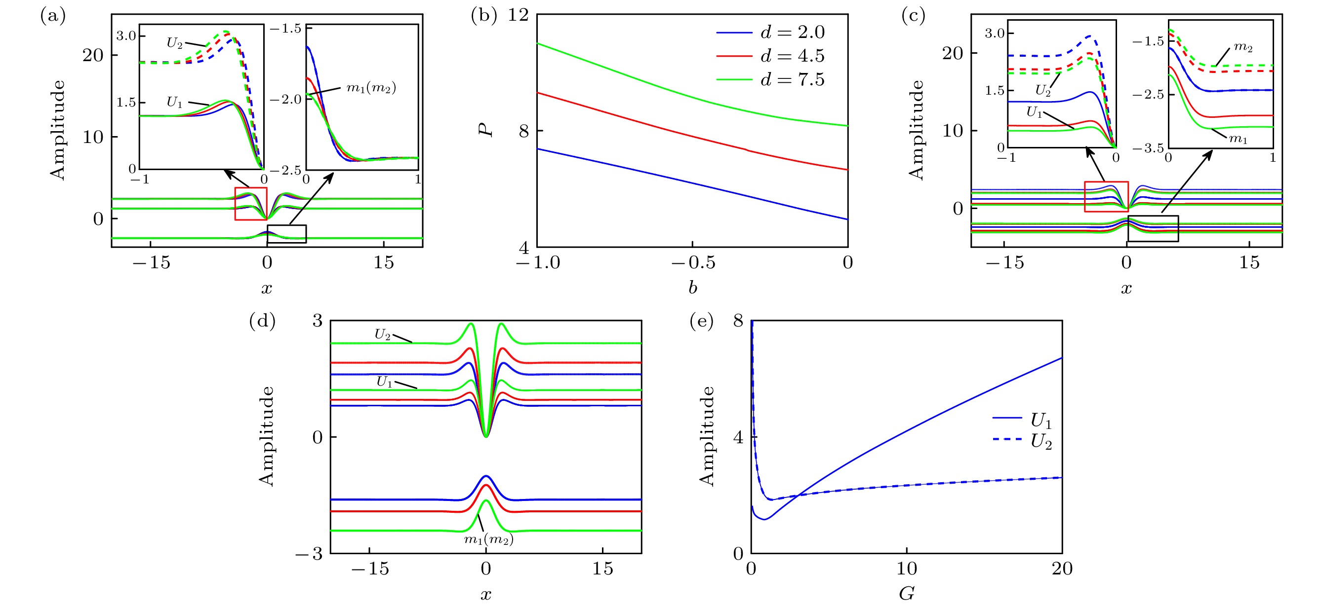 图 1 基态暗孤子数值解 (a)不同d对应的波形(


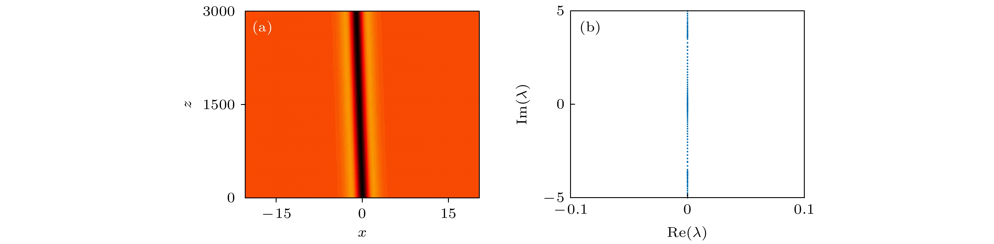 图 2 基态暗孤子的传输特征及稳定性 (a)


 图 3 偶极暗孤子的特性 (a)


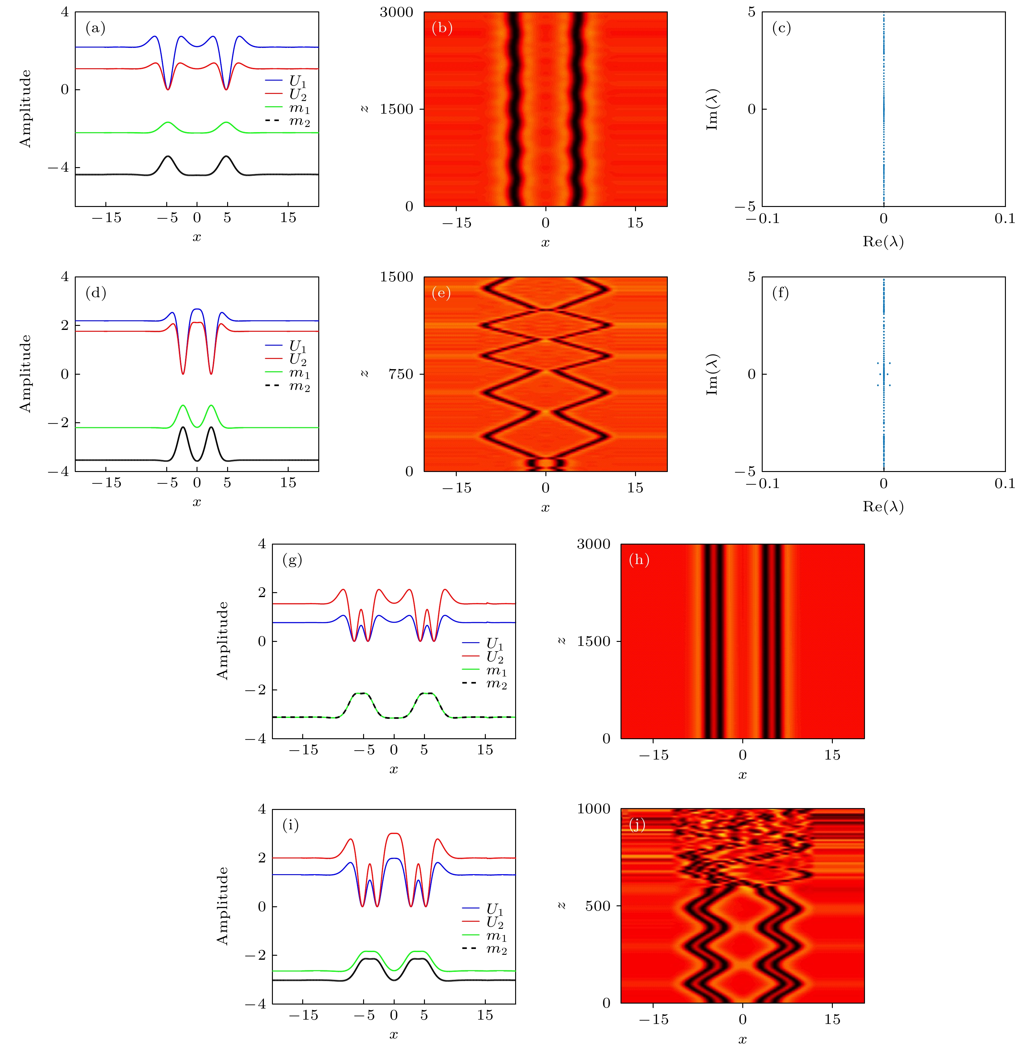 图 4 不同类型的偶极暗孤子的强度分布和传播特性 (a)?(c)分别为


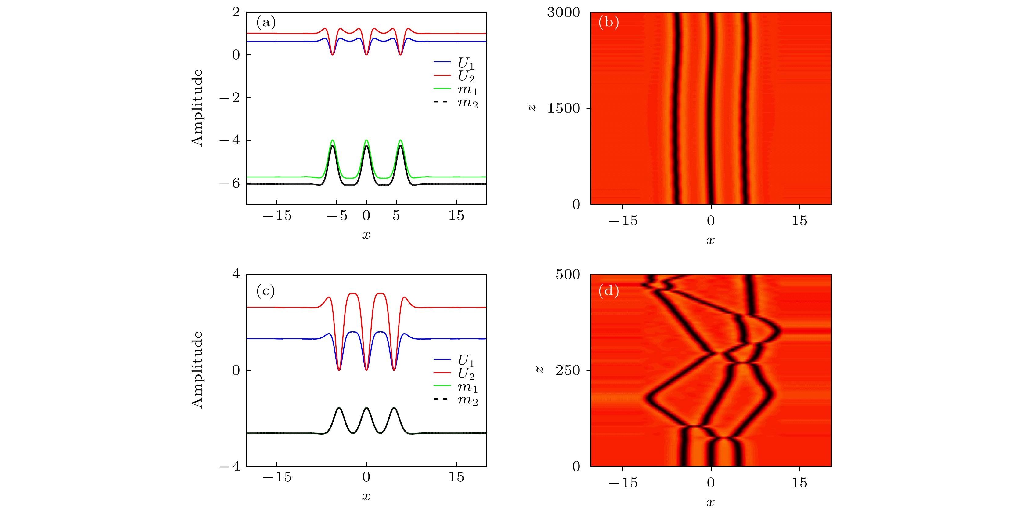 图 5 不同类型的三极暗孤子的强度分布和传播特性 (a)和(b)分别为


