摘要:本工作探索了基于Triple GEM探测器对快中子能谱的测量, 利用MCNPX和Geant4软件分别模拟了两种在Triple GEM阴极耦合由多层聚乙烯组成的堆栈式中子转化质子的转化模型, 研究对象包含了5种单能中子源和Am-Be连续谱中子源. 模拟得到了探测系统对160条单能中子的响应函数和上述源的反冲质子谱分布, 使用GRAVEL和MLEM算法对模拟得到的6种快中子源的反冲质子谱进行了解谱研究, 并把解谱结果与标准输入谱进行了对比, 结果显示与标准输入谱均符合较好, 解谱的相对不确定度为10%—15%; 并研究了气体探测器能量分辨率对解谱精度影响的关系, 结果表明微结构气体探测器的能量分辨率好于30%时, 快中子的解谱精度就可以满足实际应用需求. 本研究在以前的实验基础上提出了一种新的转化结构, 并通过模拟结果得出微结构气体探测器可以应用于快中子探测, 并能够利用得到的反冲质子谱结合合适的反演算法实现入射中子源的能谱重建. 本文积累的建模和解谱算法为将来微结构气体探测器组成的快中子探测系统应用于未知快中子源探测, 能谱重建, 实现源项识别提供了新的办法.
关键词: 中子解谱/
响应函数/
反冲质子谱/
能量分辨率

English Abstract

全文HTML

--> --> -->

中子能谱^[1,2]是每个中子源的独有特征, 可用于源项的识别^[3], 精准获得中子能谱信息在空间探测、辐射防护、核不扩散和国土安全、核材料管制等领域具有重要实际意义^[4,5]. 近十年, 国内外对中子能谱的测量进行了大量的研究. Avdic等^[6]基于液体闪烁体探测器测量了反冲质子的脉冲高度谱, 使用了非线性人工智能算法进行了解谱, 通过模拟和实验验证, 达到了识别未知中子源的目的. Hosseini等^[7]使用人工神经网络(artificial neural network, ANN)算法和改进的最小二乘法(modified least square, MLSQR)对NE-213 闪烁体探测器收集的反冲质子能谱进行了中子解谱, 论证了ANN 算法对中子解谱的适用性. Pehlivanovic等^[8]使用NE-213液体闪烁体进行了中子能谱探测研究, 使用了最大似然估计(maximum-likelihood expectation maximization, MLEM)算法和一步延时法(one step later, OSL)对反冲质子的脉冲高度谱进行了解谱, 结果表明对于连续中子源, OSL算法解谱效果优于MLEM算法. 国内在快中子解谱方面也做了一系列研究工作, 并取得了非常好的成果, 如王冠鹰等^[9]利用液体闪烁体探测器和金硅面垒探测器获得反冲质子, 并使用势能还原内点算法对中子能谱进行解谱, 该算法能够快速准确地求解中子能谱. 言杰等^[10]使用简单的不含隐藏层的线性神经网络结构, 对BC501A液体闪烁体探测器测的反冲质子谱进行了解谱, 但由于受响应函数的限制, 最后解得的能谱能点较少, 能谱数据较为稀疏, 能谱不光滑. 王冬等^[11]基于遗传算法对多球中子谱仪开展了中子解谱的仿真测试, 提出了一种由距离项和惩罚项组成的新型适应度函数, 验证了基于该新型适应度函数的遗传算法的可行性. 林存宝^[12]使用了信赖域算法对 BC501A液体闪烁体探测器测的反冲质子谱进行解谱, 得到了Am-Be, D-T和²⁵²Cf 等中子源的中子能谱. 燕奕宏等^[13]使用Bonner球谱仪测量中子源能谱, 并使用GRAVEL算法进行解谱, 中能区解谱结果与输入谱符合较好, 低能区和高能区符合较差.
综上, 当前用于中子解谱的探测器多为闪烁体探测器和Bonner球, 气体探测器应用于此方面较少, 主要是因为气体介质的能量阻止本领较低, 中子转化为质子的效率低, 导致探测效率低, 不利于中子探测.
本工作使用了一种微孔状的气体探测器-气体电子倍增器(gas electron multiplier, GEM), 1997年由欧洲核子中心CERN的Sauli^[14]研制, 具有成本低廉、耐辐照、增益高(10²—10⁶)、空间分辨率好(70 μm)^[15,16]等诸多优点, 且可以通过多层GEM膜级联的方式提高信噪比, 将GEM探测器改装成一种中子敏感的探测器, 操作比较简单. 近年来国际上虽然有多个科研机构针对基于GEM结构的中子测量进行了研究, 也取得了很好的成果^[17-20], 但大多数集中在使用含硼的转化材料提高热中子探测效率方面的研究. 本文的研究工作是利用Triple GEM探测器耦合一种新的快中子转化结构, 其将快中子转化为可直接探测的反冲质子, 而气体探测器对质子的探测效率近乎于100%, 因此可以用反冲质子数的产额表征入射中子的探测效率. 利用MCNPX和Geant4分别模拟了基于Triple GEM设计的中子探测器对不同中子源的响应, 获得了由160个单能中子响应函数组成的探测器响应矩阵, 以及探测器对Am-Be中子源的反冲质子能谱. 由于响应矩阵通常情况下为病态矩阵, 因此通过反冲质子谱求解入射中子谱(解谱)的过程实际上是求解不适定问题, 不能用直接求解的方式, 需要增加一些条件获得其近似解. 国内外研究团队发展了GRAVEL算法^[21]、最小二乘法^[22]、极大似然算法^[23](MLEM)、一步延时算法、信赖域算法和遗传算法等多种解谱算法. 本文使用GRAVEL算法和MLEM算法分别对以上模拟数据进行了联合求解, 得到了入射中子源的能谱, 并和标准能谱进行了比较.

为了实现快中子高效率的探测, 本文提出了一个堆栈式高密度聚乙烯(high density polyethylene, HDPE)快中子转化结构, 原理图如图1所示. 快中子垂直于聚乙烯薄膜进入探测器, 与其发生弹性碰撞得到反冲质子, 能量大的反冲质子逃出聚乙烯表面, 进入到气体间隔内和气体原子或分子通过碰撞电离产生电离电子, 这些电离电子通过漂移区电场的引导进入到微孔中发生雪崩效应, 最后受收集区电场的作用, 在向阳极移动过程中使阳极板产生了感应信号, 即反冲质子能量信息. 为了准确求解入射中子能谱, 探测器的响应矩阵是一个关键因素, 能否准确地获得响应矩阵将直接决定中子解谱的正确性和准确性, 由于单能中子源非常稀缺, 因此需要模拟大量的单能中子与转化结构相互作用得到响应函数, 不同能量的单能中子通过探测器后得到的反冲质子数是一一对应的, 分别对应于探测器响应矩阵中的一个元素.
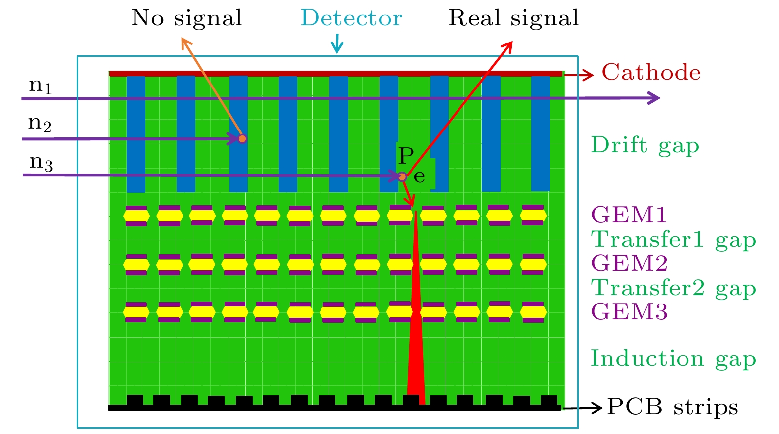图 1 中子进入Triple GEM探测器原理图(蓝色为HDPE, 绿色部分为CO₂和Ar混合气体)
Figure1. Schematic diagram of the Triple GEM-based neutron detector (The blue color is HDPE, and the green part is the mixture of CO₂ and Ar).

2

-->

2.1.堆栈式多层快中子转化结构模拟

使用MCNPX和Geant4对聚乙烯转化结构进行模拟, 主要参数为: 入射中子能量范围2—17 MeV; 入射中子数为10⁸个; 中子源距离聚乙烯薄膜距离为4 cm; 聚乙烯薄膜的密度为0.95 g/cm³.
由于快中子与聚乙烯转化结构中的氢元素发生相互作用转化为质子时会损失部分能量, 与之前入射中子相比能量减少, 若采用同一厚度聚乙烯进行转化, 可能会导致这些中子产生的质子因能量较小而不能逃出聚乙烯. 图2所示为单能中子探测效率与最优厚度之间的关系.
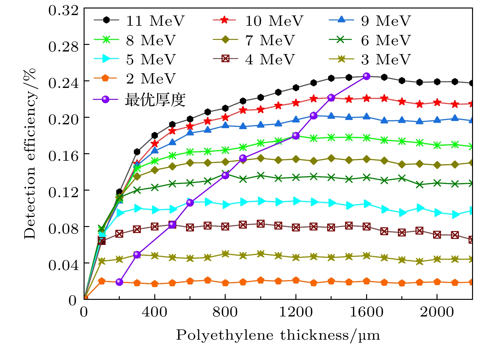图 2 不同能量的单能中子探测效率与聚乙烯厚度之间的关系及最优厚度
Figure2. The function of the detector efficiency with different polyethylene thicknesses.

图3所示为MCNPX软件对中子与聚乙烯发生弹性碰撞过程建模图, 一部分反冲质子如图中蓝色径迹所示, 其穿过聚乙烯后进入气隙内, 能量沉积在气隙间隔; 图4为MCNPX和Geant4软件模拟DT, Am-Be, DD源的探测效率的对比.
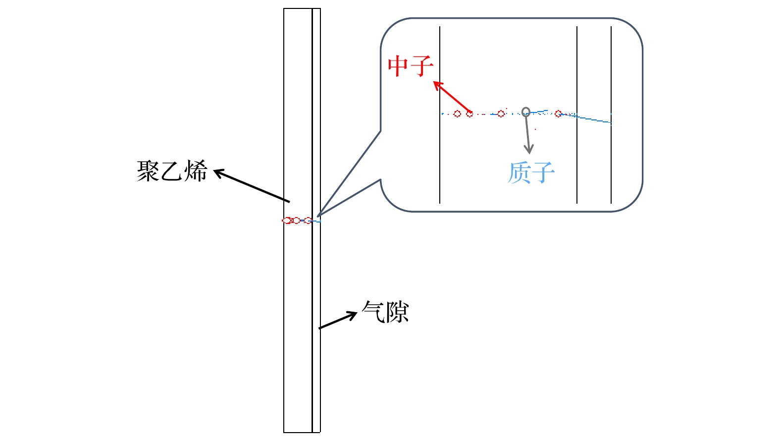图 3 中子与单层聚乙烯弹性散射图探(红色点代表中子, 蓝色为质子)
Figure3. Screenshot of the elastic collision between neutrons and polyethylene in MCNPX (the red dots represent neutrons and the blue are protons).

图 4 MCNPX与Geant4对不同中子源的测效率的模拟对比
Figure4. Simulation comparison of detection efficiency between MCNPX and Geant4 for the same thickness of polyethylene.

由图4可知, 当聚乙烯厚度较薄时, 探测效率随着厚度的增加而增加; 当厚度达到一定时, 探测效率达到最大值, 此时的厚度为最优厚度. 当厚度超过最优厚度, 探测效率趋于饱和. 实际上不管多厚的聚乙烯膜, 反冲质子仅能从聚乙烯膜表面几十个μm出射. Geant4和MCNPX对三种不同中子源与聚乙烯相互作用的最佳厚度和探测效率的模拟结果对比如表1所列.

中子源	DT			Am-Be			DD
	最优厚度/μm	探测效率/%		最优厚度/μm	探测效率/%		最优厚度/μm	探测效率/%
Geant4	2000	0.36		1200	0.12		600	0.07
MCNPX	1800	0.32		900	0.09		500	0.03

表1Geant4和MCNPX对不同中子源与聚乙烯相互作用的最佳厚度和探测效率的模拟结果
Table1.Simulation results of Geant4 and MCNPX for the optimal thickness and detection efficiency of different neutron sources interacting with polyethylene.

由于Geant4和MCNPX两者物理过程中使用的截面库和中子通量的计算方式不同, 因此探测效率会有一些差异^[24.25]. 尤其是在能量较低的区域, 探测效率相差较大, Geant4比MCNPX的探测效率在DD源处高133%, Am-Be源处高33%, DT源处高12.5%.
由于单层聚乙烯与中子发生弹性散射几率很低, 绝大多数中子会穿过聚乙烯薄膜, 为了提高探测效率, 采用多层聚乙烯结构, 以提高中子发生弹性散射的概率. 将最优厚度聚乙烯和一定厚度气隙作为一个转化单元, 根据文献[18]可知, 气体间隔采用500 μm较为合理. 中子与多层聚乙烯转化结构发生相互作用如图5所示, 反冲质子出现了小角度散射, 反冲质子径迹与中子源在同一水平线. 单元数与转化效率的关系如图6所示, 模拟结果表明DT, Am-Be和DD源的探测效率最大值分别为1.50%, 0.44%和0.14%, 此时聚乙烯转化单元均为200层左右, 比单层的探测效率高近5倍, 由此可见, 采用了多层聚乙烯的方法可以有效提高探测效率.
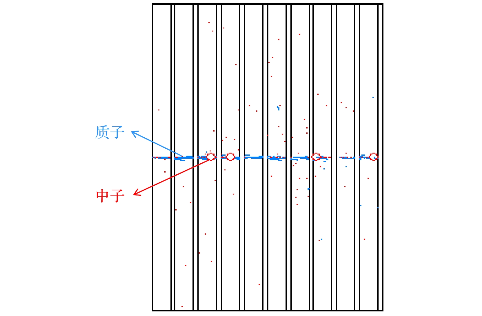图 5 MCNPX模拟的中子与多层聚乙烯相互作用(红色的点代表中子, 蓝色为质子)
Figure5. MCNPX simulated neutron interactions with multilayered polyethylene (the red dots for neutrons, the blue for protons).

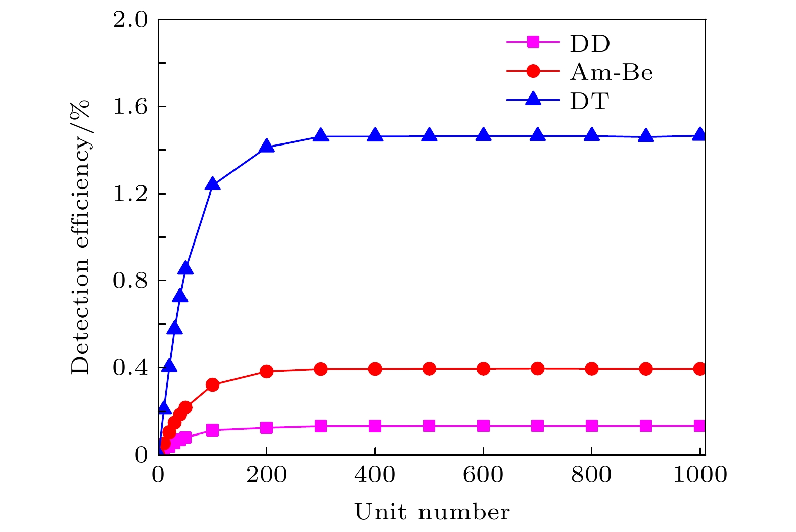图 6 多层聚乙烯结构转化效率
Figure6. Conversion efficiency of multilayer polyethylene structures.

使用MCNPX对多层聚乙烯转化结构进行了模拟, 由于初始入射中子与聚乙烯发生弹性散射产生反冲质子后会损失了一部分能量, 以致后续的聚乙烯厚度和层数不是最优, 为了获得更多反冲质子, 采用聚乙烯厚度递减的堆栈式的优化结构. 第一种模型有17个堆栈, 每个堆栈内有20层相同厚度的聚乙烯, 考虑到3D打印技术加工精度为100 μm, 因此将相邻堆栈内聚乙烯厚度按100 μm的厚度递减, 与Geant4软件模拟的结构相同^[26], 分别用M1和G1表示(下同). 为了提高反冲质子的产额, 对此提出了新的聚乙烯转化结构, 第二种模型采用了能量截断的方法, 将2—17 MeV的入射中子划分为15个间隔, 每个能量间隔为1 MeV, 求出每个能量截断值所对应的最优聚乙烯厚度及穿过的最大层数, 将每个能量间隔穿过的最大层数作为一个堆栈, 这15个堆栈组成了新的聚乙烯转化结构, 用M2表示(下同). 如图7所示, 为M2模拟的部分聚乙烯堆栈结构示意图.
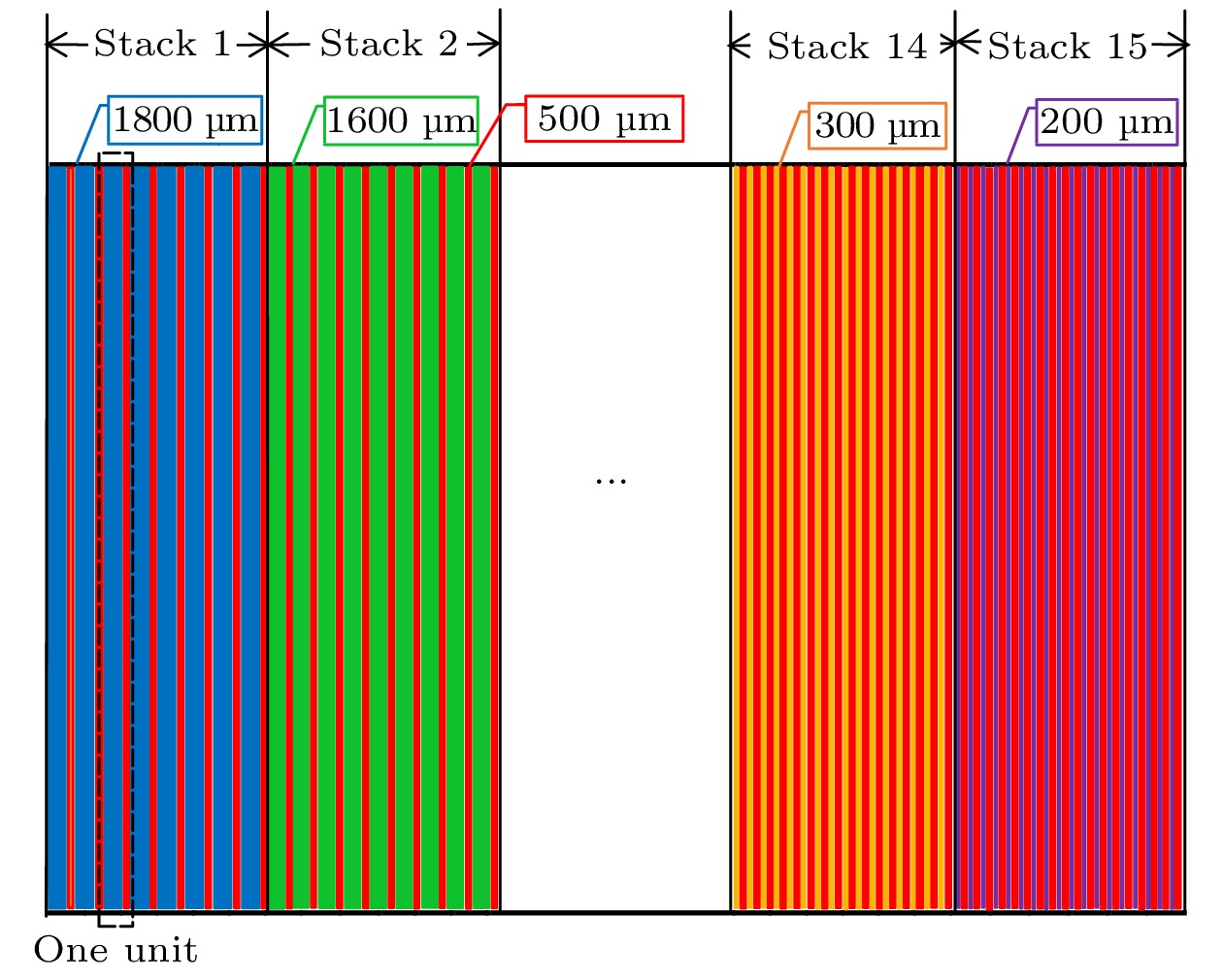图 7 M2模拟的堆栈结构示意图(蓝色、绿色、橘黄色和紫色分别代表不同厚度聚乙烯, 红色代表气隙厚度)
Figure7. Schematic diagram of the stack structure simulated by M2 (blue, green, orange, and purple represent different thicknesses of polyethylene respectively, red represents air gap thickness).

2 -->

2.2.响应函数的计算

探测器响应函数描述了入射中子能量与其引起的脉冲幅值之间的随机关系, 需要根据具体的实验条件来确定. 探测器的响应函数取决于许多可变的因素, 主要包括中子源特性以及探测器的材料组成、几何特性、工作状态和计数率等.
利用MCNPX软件对GEM探测器的响应矩阵进行模拟计算. 响应矩阵由入射的单能中子和聚乙烯转化结构相互作用后得到的反冲质子能谱组成, 将每一个入射的单能中子与其相对应的反冲质子作为一个行向量将这些向量存入一个矩阵中一行, 该矩阵即为n条行向量组成的响应函数矩阵, 共160条. 通过对响应矩阵和反冲质子谱联合求解即可得出入射中子源能谱信息, 其关系如下所示.
响应矩阵:

$\begin{split}&{{A}} = \left[ {\begin{array}{*{20}{c}} {{{{A}}_{11}}}&{{{{A}}_{12}}}& \cdots &{{{{A}}_{1m}}} \\ {{{{A}}_{21}}}&{{{{A}}_{22}}}& \cdots &{{{{A}}_{2m}}} \\ \vdots & \vdots & \ddots & \vdots \\ {{{{A}}_{n1}}}&{{{{A}}_{n2}}}& \cdots &{{{{A}}_{nm}}} \end{array}} \right],\\&{{m}} = \left[ {1,2, \cdots,170} \right],\;{{n}} = \left[ {1,2, \cdots,160} \right].\end{split}$

反冲质子能谱:

${{g}} = {\left[ {{g_1},{g_2}, \cdots,{g_n}} \right]^{\rm{T}}}.$

反冲质子谱g与响应矩阵A之间的关系可以写为下式的形式:

$\left[ {\begin{array}{*{20}{c}} {{g_1}} \\ {{g_2}} \\ \vdots \\ {{g_n}} \end{array}} \right] = \left[ {\begin{array}{*{20}{c}} {{{{A}}_{11}}}&{{{{A}}_{12}}}& \cdots &{{{{A}}_{1m}}} \\ {{{{A}}_{21}}}&{{{{A}}_{22}}}& \cdots &{{{{A}}_{2m}}} \\ \vdots & \vdots & \ddots & \vdots \\ {{{{A}}_{n1}}}&{{{{A}}_{n2}}}& \cdots &{{{{A}}_{nm}}} \end{array}} \right] \cdot \left[ {\begin{array}{*{20}{c}} {{f_1}} \\ {{f_2}} \\ \vdots \\ {{f_m}} \end{array}} \right], $

其中f即为所求入射中子谱的能谱信息.
图8仅展示了16条整数单能中子的响应函数. 使用的入射中子能量为2—17 MeV, 入射中子能量间隔为0.1 MeV, 因此得到了${\rm{160}} \times {\rm{170}}$的响应矩阵. 由于模拟单能中子的能量间隔小, 在解谱时便于区间划分, 得到的响应函数越精细, 求解得出的中子谱的点越密集.
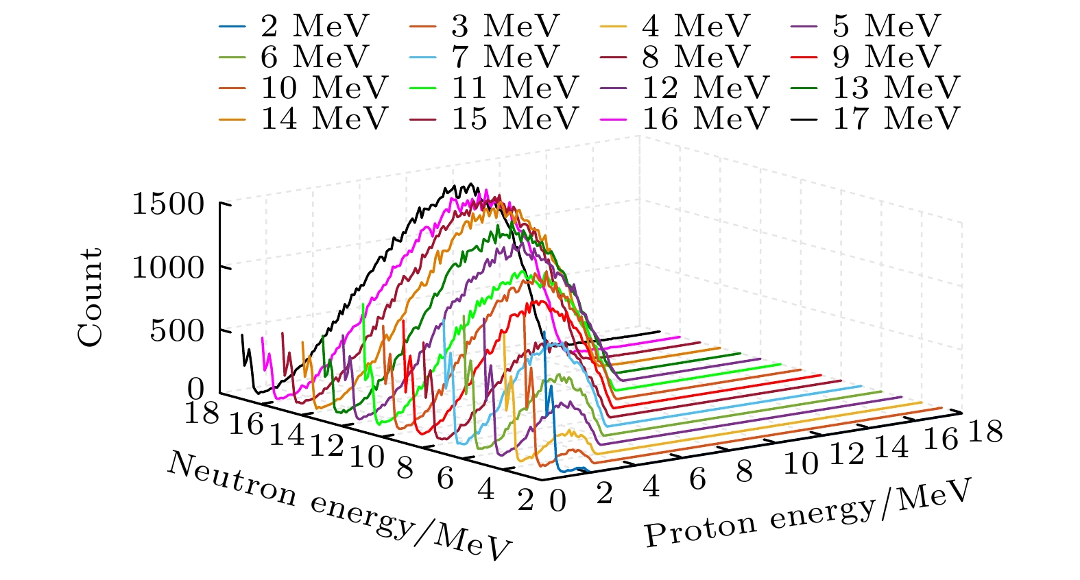图 8 不同中子源对应的响应函数
Figure8. Response functions corresponding to different neutron energies.

2

-->

3.1.GRAVEL解谱算法

GRAVEL解谱算法由SAND-Ⅱ算法演化而来, 是最早由德国 PTB 实验室提出的一种交互式迭代算法, SAND-Ⅱ常用于反冲质子解谱, 其迭代公式为

$f_j^{k + 1} \!=\! f_j^k\exp \!\left[\! {\frac{{\displaystyle\sum\limits_j {W_{ij}^k} \ln \left(\! {{g_i} \Big/\displaystyle\sum\limits_j {{A_{ij}}\exp \left( {\ln f_j^k} \right)} } \!\right)}}{{\displaystyle\sum\limits_j {W_{ij}^k} }}} \!\right], $

$W_{ij}^k = \frac{{{A_{ij}}f_j^k}}{{\displaystyle\sum\nolimits_j {{A_{ij}}f_j^k} }} \cdot \frac{{g_i^2}}{{\sigma _i^2}}.$

式中, ${f_j}$是入射中子在j能量区间的辐射强度; ${f^k}$为第$k$次迭代得到的第j个能量间隔的辐射强度, 当$k$为0时, 初始中子谱常取常数谱; ${A_{ij}}$是第i个脉冲幅度间隔与第j个能量区间的耦合的响应函数; $W_{ij}^k$是权重因子; ${g_i}$是第i个脉冲幅度处的强度, ${\sigma _i}$为${g_i}$的统计误差, 一般为${g_i}$的平方根, 若${g_i}$的数值为0, 则${\sigma _i}$取1. GRAVEL具有对初始值不敏感, 解为非负值且噪声小等优点, 缺点是解不完全收敛, 迭代次数越多, 越容易发散.
2 -->

3.2.MLEM算法

MLEM算法是利用样本结果信息, 反推最大概率导致这些样本结果出现的模型参数值. 理论上, 质子和中子谱均为连续函数, 测量装置允许在有限的多个点测量质子能谱的值. 因此将实轴划为有限的多个能量区间, 区间越小, 落在区间的粒子数具备泊松分布, 且相互独立.

$f_i^{k + 1} = f_i^k\sum\limits_j {\dfrac{{{g_j}{A_{ij}}}}{{\displaystyle\sum\limits_l {f_l^k{A_{jl}}} }}}. $

MLEM算法具有以下特点: 算法收敛, 对于每个k, 总有$l({f^k}) < l({f^{k + 1}})$. 若初始值${f^0}$非负, 那么整个响应矩阵A和质子谱g均是非负, 所有的解${f^k}$也都为非负. 对于每个近似的${f^k}$总有

$\sum\limits_i {f_i^k} = \sum\limits_j {{g_j}}.$

由此可见, 脉冲总和保持不变, 只在不同能量组中重新分配.

2

-->

4.1.单能中子源解谱

通过对单能入射中子得到的反冲质子谱的电离过程进行模拟, 得到反冲质子在气隙(气体成分为70% Ar和30% CO₂)中的沉积能量, 如图9所示. 随着入射中子能量增加, 反冲质子最大概率沉积的能量(峰位所对应的能量)逐渐减少, 这主要是由于气隙间隔固定(500 μm), 远小于质子在气体中完全沉积时所穿行的距离, 因此低能质子更容易沉积到气隙里. 图10显示了入射中子能量与反冲质子沉积能量峰位的关系.
图 9 不同入射中子对应的反冲质子在气隙中的沉积能量
Figure9. Deposition energy of recoil protons in the air gap corresponding to different incident neutrons.

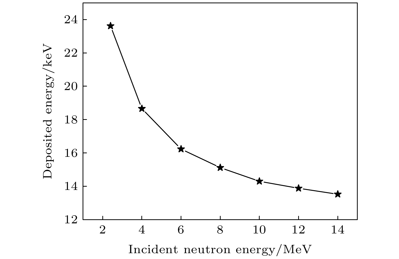图 10 入射中子能量与反冲质子沉积能量关系
Figure10. Relationship between neutron incidence energy and recoil proton deposition energy.

图11为使用两种算法分别对Geant4软件和MCNPX软件的模拟数据进行解谱的结果. 将沉积能量与响应矩阵联合求解得到单能入射中子源的能谱信息. 从图11中可知, 两种算法都正确地预测了能量分辨率约为0.1 MeV的中子的解谱能量, 但其峰值强度高低不等, 以峰值强度最大值为标准进行归一化处理. 在4 MeV处的峰值与参考数据相匹配, 但在2.4, 8.0, 12.0和14.0 MeV处的峰值分别低估了32%, 15%, 5%和20%, 这因为在解谱算法中, 在峰值处出现了不同程度的能谱展宽.
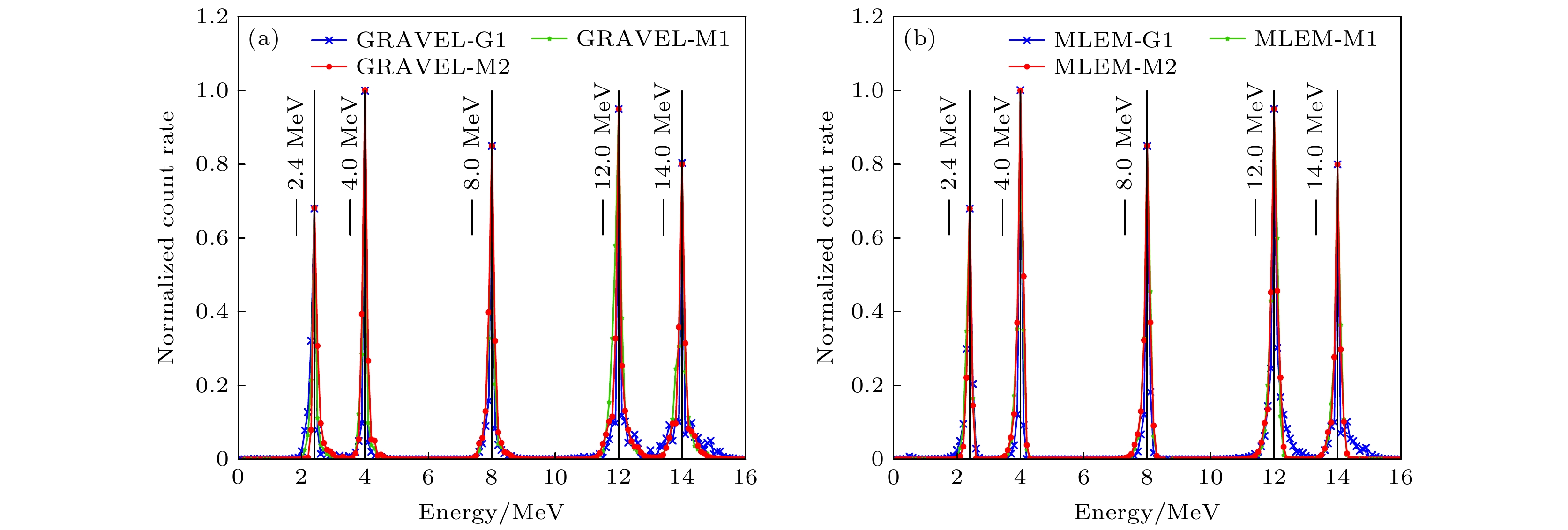图 11 两种算法对Geant4软件和MCNPX软件模拟数据的解谱结果　(a) GRAVEL算法对单能中子解谱图; (b) MLEM算法对单能中子解谱图
Figure11. Results of two algorithms for solving the spectrum of simulated data from Geant4 software and MCNPX software: (a) GRAVEL algorithm on single-energy neutron unfolding spectra; (b) MLEM algorithm for single-energy neutron unfolding spectra.

2 -->

4.2.连续中子源解谱

当入射源为Am-Be源时, 通过GRAVEL算法和MLEM算法对模拟的探测器的响应矩阵和脉冲幅度谱进行解谱, 解谱的结果如下图12所示.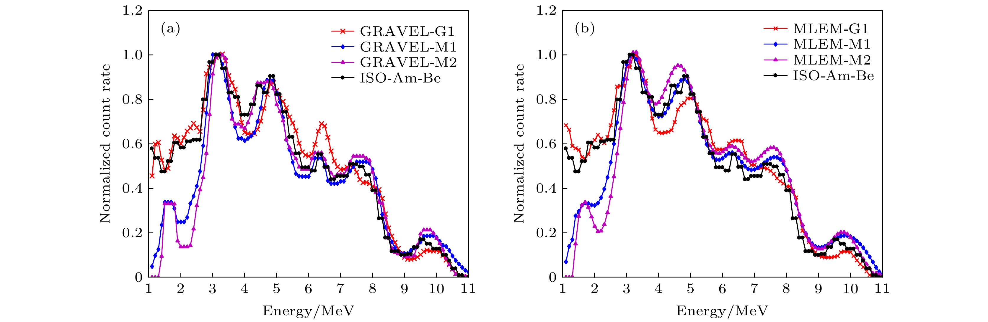
图 12 两种解谱算法对Geant4软件和MCNPX软件模拟Am-Be源的解谱结果　(a) MCNPX与Geant4基于GRAVEL算法的解谱结果; (b) MCNPX与Geant4基于MLEM算法的解谱结果
Figure12. Results of the unfolding of the simulated Am-Be sources by two solution algorithms for Geant4 software and MCNPX software:　(a) Unfolding results of MCNPX and Geant4 based on GRAVEL algorithm; (b) unfolding results of MCNPX and Geant4 based on MLEM algorithm.

从图12可以看出, GRAVEL算法和MLEM算法均可以用于Am-Be源的解谱, 两种算法解谱的峰位均与输入谱符合较好.
G1结构解谱结果表明, GRAVEL算法在低能区出现较大幅度振荡, 在中高能区振荡幅度较小, 这是由于GRAVEL算法的解不完全收敛, 因此会出现不同程度的能量展宽. MLEM算法则比较平滑, 可见MLEM算法抗干扰能力强于GRAVEL算法. MLEM算法与输入谱相比, 整体符合较好.
对M1结构和M2结构解谱, 两种算法在2.7—11.0 MeV与标准谱符合较好, 但在1.0—2.6 MeV处的值低于输入中子谱在该范围内的值, 由此可见, MCNPX更适合模拟中高能区中子.
使用气体探测器对⁵⁵Fe低能的5.9 keV的X射线测量的能量分辨率的好于15%. 现将探测器应用于反冲质子的测量, 通过模拟沉积能量峰值为13.8 keV的反冲质子在探测器内部电离作用以及电离电子在GEM孔内雪崩效应, 得到了探测器的能量分辨率为13.4%, 如图13所示, 相比于对X射线的测量, 能量分辨率得到改善和提高, 因此Triple GEM结构的中子探测器在中子探测及测量方面应用是可行的.
图 13 反冲质子在气体探测器中的能量分辨率
Figure13. Energy resolution of recoil protons in gas detectors.

为了使基于气体探测器的中子探测系统能给将来的实验提供更可靠的参考, 本工作在模拟仿真时考虑了气体探测器的能量分辨率对解谱精度的影响, 模拟时采用的气体探测器的能量分辨率为10%—30%, 如图14所示, 结果表明探测器的能量分辨率越小, 求解的中子谱的相对不确定度就越小, 结果越准确. 同为MCNPX软件模拟的两种不同模型之间, 相对不确定度随着能量分辨率变差而逐渐增大, 且趋势大致相同. Geant4模拟结果解谱的相对不确定度在能量分辨率为10%—18%时为均匀增加, 在能量分辨率大于18%时, 相对不确定度扩大了1%. 两种不同的变化趋势原因在于两者模拟结果数据的不同, Geant4模拟结果为单个粒子数分别耦合能量分辨率的高斯分布, 然后对其进行不同能量间隔的划分, 因此随着能量分辨率不断变差, 能谱的展宽程度愈加剧烈, 导致相对不确定度不是均匀变化. 而MCNPX模拟结果则先进行能量区间划分, 然后再耦合关于能量分辨率的高斯分布, 因此, MCNPX的相对不确定度为均匀变化. 对于同一软件或模型, GRAVEL算法和MLEM算法解谱结果的相对不确定度相差不大, 约为0.2%.
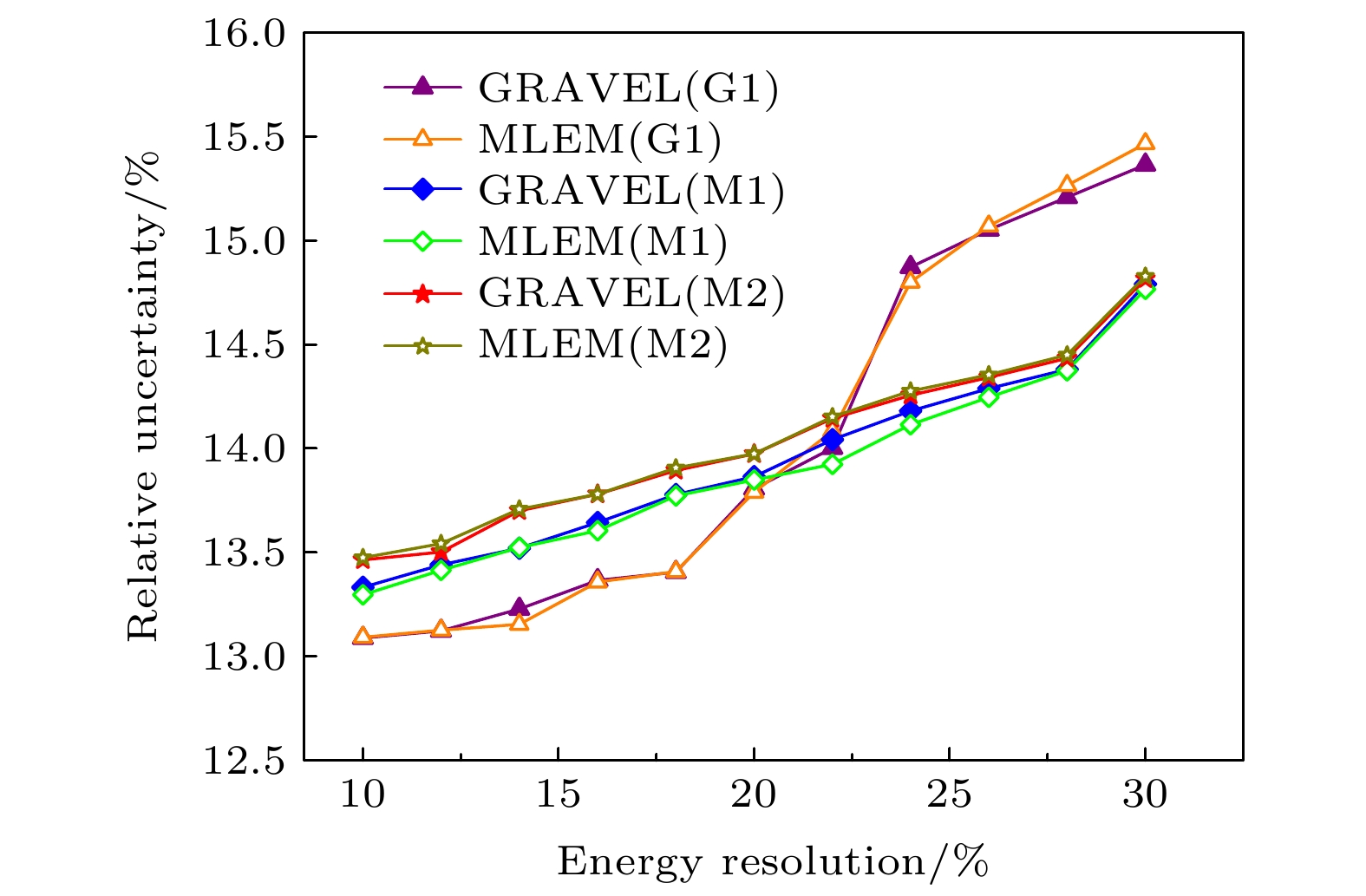图 14 相对不确定度与能量分辨率的关系
Figure14. Plot of relative uncertainty versus energy resolution.

为了准确地评价两种算法对MCNPX的两种结构和Geant4的结构模拟结果的求解效果, 分别用均方误差(mean square error, MSE)表征预测的中子谱和真实中子谱之间的差异程度, 理想状态下接近于0, 平均相对偏差(average relative deviation, ARD)表示预测的中子光谱与真实中子能谱之间的偏差程度, 中子能谱质量(quality of neutron spectrum, Qs)表示预测的中子谱与真实中子谱的接近程度. 作为评价解谱结果误差水平的标准, 公式如下所示:

${\rm{MSE}} = \frac{1}{n}\sum\limits_j^n {{{\left( {{f_j} - f_j'} \right)}^2}}, $

${\rm{ARD}} = \frac1{n}{{\left( {\displaystyle\sum\nolimits_j {\frac{{\left| {{f_j} - f_j'} \right|}}{{f_j'}}} } \right)}}, $

${\rm{Qs}} = {\left[ {\frac{{\displaystyle\sum\nolimits_j {{{\left( {{f_j} - f_j'} \right)}^2}} }}{{\displaystyle\sum\nolimits_j {{{\left( {f_j'} \right)}^2}} }}} \right]^{\tfrac{1}{2}}}, $

其中${f_j}$为所求的入射中子谱解谱结果; $f_j'$为标准中子源. 对MCNPX两种结构和Geant4模拟的结果进行误差分析, 并列于表2中.

	G1			M1			M2
	MLEM	GRAVEL		MLEM	GRAVEL		MLEM	GRAVEL
MSE	0.48%	0.65%		2.1%	2.4%		1.4%	1.8%
ARD	18.00%	19.00%		21.0%	22.0%		20.0%	21.0%
Qs	12.00%	14.00%		28.0%	30.0%		19.0%	21.0%

表2MCNPX两种结构和Geant4模拟结果经MLEM算法和GRAVEL算法解谱后误差水平
Table2.Error levels of the two MCNPX structures and Geant4 simulation results after unfolding by the MLEM and GRAVEL algorithms.

由表2可得G1比M1的解谱结果在MSE, ARD和Qs三个误差方面分别好1.7%, 3%和16%. 造成这种误差的原因主要在于MCNPX在低能区1.0—2.6 MeV模拟结果较差; M2比M1的解谱结果在MSE, ARD和Qs三个误差方面分别好0.7%, 1%和9%. 由于两种结构响应函数不同, M2在低能区可以获得更多的反冲质子, 因而对于低能区解谱结果略好于结构M1. 比较GRAVEL算法与MLEM算法的解谱结果, GRAVEL算法比MLEM算法在MSE, ARD和Qs分别高约0.3%, 1.0%和2.0%, 误差是由于GRAVEL算法解谱结果在低能区存在较大振荡, MLEM算法解谱结果相对平滑所致.

本工作利用MCNPX和Geant4软件对基于Triple GEM结构快中子探测器阴极转化结构进行了研究模拟, 获得了该转化结构对应的响应函数矩阵, 由于响应矩阵为病态矩阵, 因此响应矩阵和脉冲幅度谱之间微小的变化都会导致解谱结果和输入谱有很大偏差. 通过利用GRAVEL算法、MLEM算法对M1, G1和M2的模拟数据进行了解谱. 解谱结果表明, 两种算法在Triple GEM结构快中子探测器的解谱过程中均有很好的效果. GRAVEL算法在求解低能部分时存在解谱精度低, 结果不稳定, 有较大幅度的振荡. MLEM算法解谱精度相较于GRAVEL算法高, 且解谱曲线更加平滑, 与输入谱符合较好, 是一个实用的中子解谱方法. 两种蒙特卡罗软件, 对于单能中子源模拟均比较准确, 可以用于对未知中子源的模拟. 对于连续中子源, Geant4的低能部分精确度相较于MCNPX要高. MCNPX软件更适合用于中高能中子的模拟. 本工作完成了MCNPX对于探测器结构的模拟与中子能谱解谱的计算, 后续将展开相关实验, 进一步探究探测器转化结构对于解谱的精度的影响, 并考虑低能部分用G4模拟, 中高能部分用MCNPX模拟.