摘要:超短超强激光因其极端的物理参数范围以及可用于研究相对论等离子体等特征, 成为当前激光驱动磁重联物理的研究热点. 通常采用两路激光与平面靶相互作用实现激光驱动磁重联, 然而在实验诊断中, 由于激光等离子体自身的复杂性导致很难辨别磁重联的物理特征. 本文对两路短脉冲激光驱动平面靶磁重联进行了数值模拟, 重点分析了靶后电势分布特征和磁重联之间的关系. 模拟结果显示, 靶后电势分布可以直接影响被加速离子在探测面上的空间分布, 因此可用来直接诊断短脉冲激光驱动磁重联实验.
关键词: 电势分布/
数值模拟/
磁重联/
短脉冲激光

English Abstract

全文HTML

--> --> -->

磁重联是等离子体物理中一个基本而又重要的物理过程, 它能够将等离子体存储的磁能转换为等离子体的热能或动能. 高速准直的喷流、等离子体的快速加热以及加速产生的高能粒子是磁重联过程的主要特征, 并广泛存在于天体和实验室等离子体中, 如太阳耀斑和日冕物质抛射^[1], 蟹状星云中的伽马射线耀斑^[2], 磁星的巨型耀斑^[3], 活动星系核中的相对论性喷流等, 以及激光驱动的等离子体准直喷流^[4], 磁重联中的非热粒子加速^[5]等.
实验室中可以通过构造磁场拓扑结构来研究磁重联演化过程^[6,7], 进而理解天体等离子体现象. 天体等离子体和实验室等离子体在物理上有许多相似之处, 但两者在尺度上存在巨大的差异, 通常利用标度变换^[8]来建立两者之间的联系. 近年来, 利用激光与固体靶相互作用来驱动磁重联的方式, 极大地扩展了磁重联研究的物理参数范围. 在不同激光脉宽驱动产生的磁重联实验中, 为了研究磁重联通常需要使用不同的诊断技术. Nilson等^[6]和Willingale等^[7]利用Vulcan装置的纳秒长脉冲激光进行了磁重联实验, 前者通过光学探针和汤姆孙散射两种诊断分别获得了喷流的速度和重联区的电子温度, 实现了两束激光驱动磁重联的实验, 后者通过质子成像结果研究了磁重联过程. Zhong等^[9]利用神光Ⅱ高功率纳秒长脉冲激光装置再现了Masuda等^[10]在太阳耀斑中观测到的环顶X射线源.
超短超强激光与物质相互作用能够驱动产生超强磁场, 可以构建出与极端相对论性天体相似的物理环境. Wagner等^[11]在实验室用超短脉冲激光实现了百兆高斯量级的强磁场, 为在实验室研究极端天体物理问题提供了更大的可能性. Raymond等^[12]在OMEGA EP激光装置上进行了皮秒短脉冲激光驱动相对论性磁重联的实验, 分别通过铜K_α源成像和电子谱仪得到了相对论性电子的能量分布及能谱变化, 这些诊断结果初步验证了实验过程中磁重联的发生. 然而对于实验中产生的非热电子来源, 是激光自身产生的相对论性电子还是重联加速的电子, 还需要进一步区分. 目前利用飞秒超短脉冲激光和等离子体靶相互作用驱动磁重联的实验很少, 主要还是以数值模拟研究为主. Ping等^[13]通过数值模拟研究了飞秒激光驱动产生的磁重联, 发现强激光驱动产生的磁重联的重联率远高于经典理论给出的重联率. Gu等^[14]通过模拟发现飞秒激光驱动的磁重联能够高效地将磁能转化为电子的动能. Guo等^[15,16]分析了相对论性磁重联中的粒子加速问题, 提出了磁重联产生硬幂律能谱的前提条件, 认为大尺度上的相对论性磁重联中的主要加速机制是费米加速. 相对论性磁重联中的粒子加速机制仍有很多未解决的问题, 比如电流片的撕裂不稳定性、外加引导磁场、作用区域的尺度等也都是相对论性磁重联中的研究热点^[17]. 目前利用短脉冲激光驱动的磁重联实验较少, 为研究极端相对论磁重联, 除了进行更多的短脉冲激光驱动磁重联的实验外, 还需要提高实验诊断技术, 发展实验诊断方案来获得更加详细的实验数据.
本文使用相对论性的Particle-in-Cell (PIC)计算程序EPOCH^[18], 模拟了短脉冲激光和固体平面靶相互作用的过程, 其中分别使用了单束激光和两束激光进行了对比, 重点分析靶后电势的分布特征. 结合模拟结果和相关的实验数据, 提出通过电势分布来判断磁重联的发生. 本文第1部分详细说明了数值模型中使用的参数设置; 第2部分深入分析了靶后电势和磁重联之间的联系, 并给出了我们的结论和推论; 第3部分给出了本文的结论.

本文使用EPOCH程序^[18]分别模拟了单束激光和两束激光作用在固体平面靶上的过程. PIC方法是一种能够自洽地模拟大量粒子在外场及自场中运动的数值计算方法. 本文的模拟结果都是基于二维的PIC数值模拟所得到的, 下面将详细介绍模拟中的初始参数设置.
模拟区域中激光和固体平面靶的设置如图1所示, 在模拟的初始时刻t = 0, 激光从模拟区域最左侧垂直入射到固体平面靶上. 模拟设置的盒子大小为L_x = 27 μm和L_y = 80 μm, 使用的初始粒子总数为9.6 × 10⁷个. 模拟区域的空间分辨率为0.02 μm, 固体平面靶的趋肤深度${l_{\rm{s}}} = {c / {{w_{{\rm{pi}}}}}} = $$ {c / {\sqrt {{{{n_{\rm{i}}}{e^2}} / {{\varepsilon _0}{m_{\rm{i}}}}}} }} \approx$2.6 μm, 所以该分辨率用于研究离子效应是足够的. 入射激光强度的峰值为6 × 10¹⁹ W/cm², 脉宽为350 fs, 激光波长为1 μm. 固体平面靶表面入射点的激光焦斑直径为6 μm, 其中两束激光的中心间距为12 μm. 模拟使用的固体平面靶的尺寸为l_x = 15 μm和l_y = 80 μm, 固体平面靶由中性铜原子构成, 初始温度为0 K, 初始密度为50n_c (其中临界密度${n_c} = {{{\omega ^2}{m_0}{\varepsilon _0}} / {{e^2}}}$, 激光频率$\omega = {{2{\text{π}}c} / \lambda }$, λ为激光波长). 模拟过程中, 为铜原子设置了3个电离能级(7.73, 20.29, 36.84 eV), 吸收了额定的能量之后, 铜靶中的铜原子将发生离化产生电子和离子, 因此电子数会随着激光和固体平面靶的相互作用而不断增加. 模拟过程中, 对粒子使用了开放边界条件, 对电磁场使用了吸收边界条件. 模拟每次完成10 fs的运算后, 会对该时间段内每个步长产生的数据取算术平均(即取时间平均), 这个对时间取平均后的结果就是我们最后得到的模拟数据.
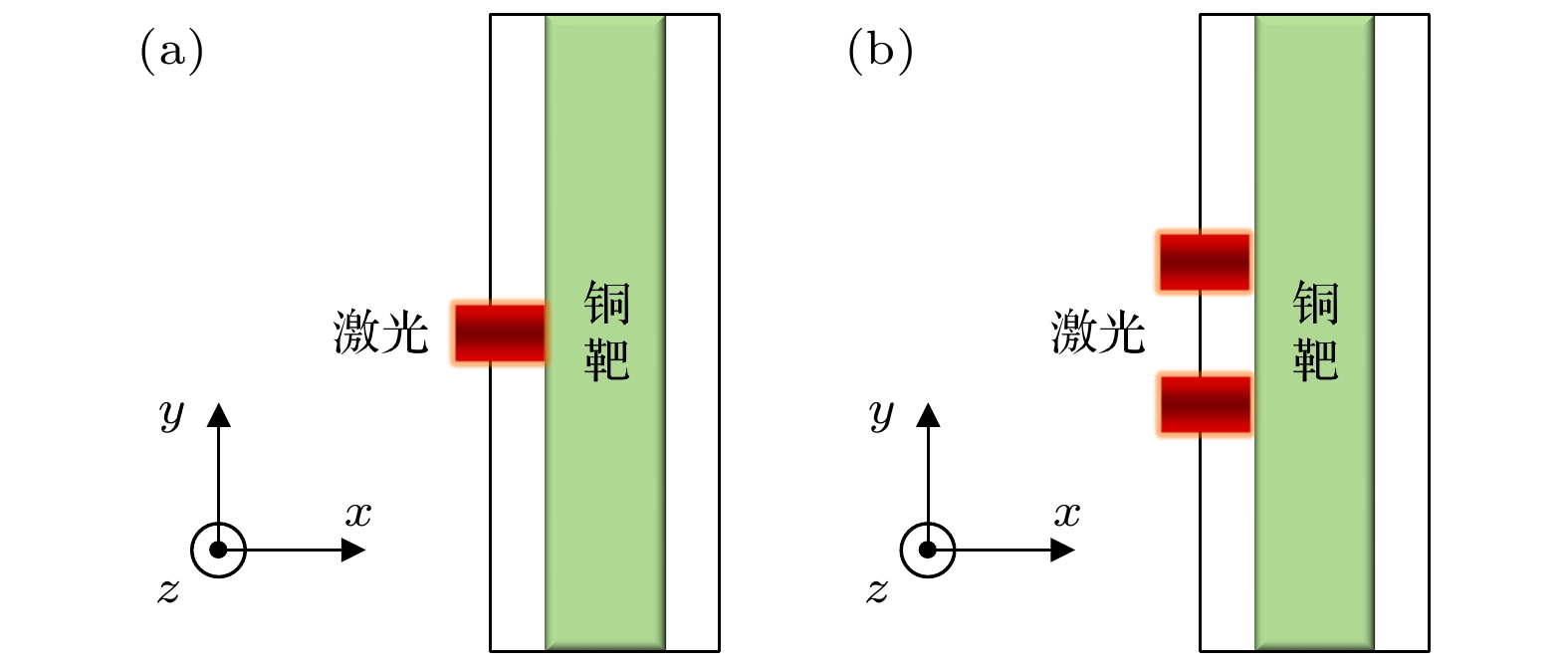图 1 模拟区域内的激光和固体平面靶(黑色线框为模拟区域)　(a) 单束激光; (b) 两束激光
Figure1. Lasers and solid planar target in the simulation box (black wireframe serves as the simulation box): (a) Single laser; (b) two lasers.

激光作用到固体平面靶上会电离出大量电子, 同时电子会在激光与靶相互作用过程中被加速, 所产生的高能电子会进入靶的内部以及其他真空区域^[19]. 随着靶后电子的增加, 这些电子会在德拜长度范围内形成电荷分离场, 该电场可以电离靶面原子并加速电离出的质子或离子, 这种加速方式称为鞘层加速^[20]. 被加速的质子会向靶后运动, 实验上可以通过靶后的辐射变色膜片(RCF)成像记录这些质子的空间分布^[21], 下面将分析靶后电势分布的特征及其与磁重联之间的联系.
首先, 通过分析靶前与靶后的重联电场变化曲线来研究磁重联的发生情况, 根据模拟结果得到了如图2所示的两束激光中的重联电场及单束激光中的鞘层电场分布. 单束激光中的鞘层电场是对初始数据乘以2得到的, 靶前鞘场数据是从矩形[(3 μm, –5 μm), (6 μm, –7 μm)]中取得的, 靶后鞘场数据是从矩形[(21 μm, –5 μm), (24 μm, –7 μm)]中取得的. 两束激光中的重联电场的数据取样区域分别为: 靶前[(3 μm, 1 μm), (6 μm, –1 μm)]; 靶后[(21 μm, 1 μm), (24 μm, –1 μm)]. 为了保证在对比两个模拟中的电场强度时具有相同的激光输入能量, 所以加倍了单束激光中的鞘层电场. 从图2可以发现, 两束激光中的重联电场强度存在上升和下降的过程, 这初步说明了磁重联的发生. 如果对比两者的电场曲线可以发现, 两倍单束激光中的鞘层电场比两束激光中的重联电场要强, 说明磁重联过程对靶后鞘层电场产生了明显的减弱作用. 通过对电场进行空间上的积分, 可以研究靶后电势的空间分布特征, 进而研究靶后离子的空间分布.
图 2 (a) 靶前和(b) 靶后的鞘层电场E_x随时间的变化
Figure2. Sheath electric field E_x curves over time at (a) the front target and (b) the rear target.

靶后电势分布可以反映空间中电磁场对离子的加速情况, 下面根据电场强度E_x得到了靶后电势的分布曲线. 考虑到等离子体的德拜屏蔽效应, 利用公式${\lambda _{\rm D}} = {\left[ {{{k{T_e}} / {\left( {4\pi n{e^2}} \right)}}} \right]^{{1 / 2}}}$计算出德拜长度${\lambda _{\rm D}} \approx$1 μm (其中温度kT_e和数密度n分别取6 MeV和7 × 10²⁰ cm^–3), 所以电势积分范围选在了靶后1 μm内的区域. 模拟区域的网格长度为0.02 μm, 然后利用电势公式$\Delta \varphi = \displaystyle\int_{{x_1}}^{{x_2}} {{E_x}{\rm d}l}$(其中${x_{\rm{1}}} =$21 μm, ${x_{\rm{2}}} = $22 μm)对靶后1 μm内的区域进行积分. 考虑到靶后离子加速是一个持续的过程, 需要对整个过程的电势取时间平均值, 这里取6 MeV离子经过长度${\lambda _{\rm{D}}} \approx$1 μm 所需要的时间. 通过计算可以得到时间范围${t_0} \approx 90\;{\rm{ fs}}$. 分别对两个模拟中的靶后电场达到最大值之后的90 fs内的电势取平均, 图3(a)是对时间取平均之后电势的计算结果, 计算积分使用的数据取在了420—510 fs之间. 蓝线的电势曲线双峰对应了靶后离子堆积的两个区域, 该电势分布曲线和Sentoku等^[21]在相似模拟参数下得到的电势分布曲线是一致的, 并且电势的分布特征和Sentoku单路激光实验的质子成像结果符合得很好, 即双峰电势分布和RCF成像中的环状结构. 观察图3(a)中的橙线, 能够看到曲线中的两个峰值中间还存在着一个峰值, 这种三峰值的分布特征在靶后则对应了3个离子堆积区域. 两个激光焦斑位置处产生的等离子体会由于膨胀碰撞而在中轴处形成粒子聚集区域, 但由于等离子体整体电荷呈中性, 对靶后电势影响较小, 所以我们认为等离子体间的碰撞对靶后电势分布的影响可以忽略. 图3(b)给出了靶前磁重联的示意图, 受磁重联影响的靶前电子穿过固体平面靶进入靶后区域, 和靶后由于磁重联产生的电子共同产生鞘层电场加速中轴处的离子. 这可以解释两束激光中靶后电势曲线中轴处出现的第3个峰值, 因此我们认为可以通过靶后电势分布特征来判断磁重联的发生. 在单束激光和平面靶相互作用的实验中, 靶后质子成像呈现一个环状结构, 对应了靶后电势分布的两个峰值; 而在两束激光和平面靶相互作用的实验中, 我们认为磁重联发生之后靶后质子成像图像会出现两个并列的环, 对应的则是靶后电势曲线上的3个峰值. 由于磁重联的时间是有限的, 所以在不同的时间对靶后离子分布进行统计, 得到的离子分布也会存在显著差异.
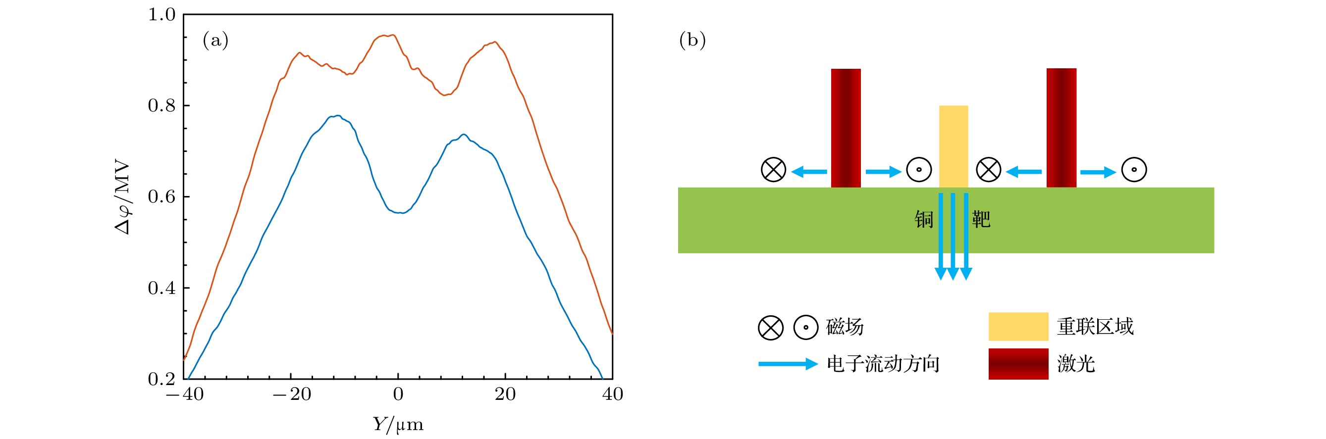图 3 (a) 单束激光(蓝色)和两束激光(橙色)对时间取平均后得到的靶后电势分布; (b) 磁重联过程的示意图
Figure3. (a) Electric potential distribution averaged over certain time at the target back obtained from the data of single laser (blue line) and two lasers (orange line) respectively; (b) the illustration of magnetic reconnection process.

为了更加直观地验证上面的结论, 对模拟中的靶后特定能量的离子进行了统计. 对所有时间上靶后3 μm处固定能量离子的空间分布进行叠加, 叠加后得到的统计结果如图4所示. 由于离子运动到靶后一定距离(10 μm或者更远)耗时比模拟设定的时间要长的多, 所以这里统计的是1800 fs内离子的累积分布情况. 受限于当前的计算能力, 模拟过程无法使用太多的虚拟粒子进行计算, 所以最后模拟中统计到的数据有很强的离散性. 通过对有限的模拟数据进行拟合得到了黄色曲线的分布, 采用光滑样条(smoothing spline)拟合的相关系数约为0.65. 拟合结果的分布特征反映出, 磁重联影响下的靶后电势分布对靶后离子分布存在显著影响. 图4(a)是单束激光情况下的统计结果, 4.5 MeV离子主要分布在中心两侧区域, 符合前面电势分布的双峰结构特征, 值得一提的是能量更高的离子则不存在类似的空间分布特征. 图4(b)是两束激光情况下的统计结果, 6 MeV离子主要分布在中心及其两侧的区域, 这个统计结果也符合前面的结论和猜测, 同样对于能量更低的离子也不存在相似的空间分布特征. 这个统计结果更加直观地验证了前面分析的结论和想法.
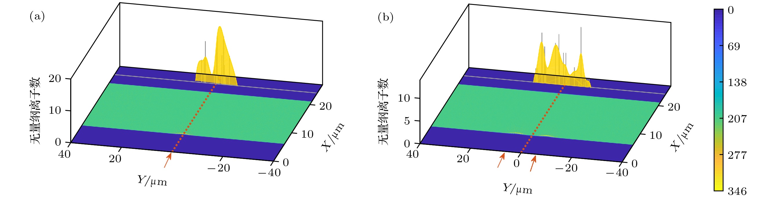图 4 靶后离子分布的统计结果(灰色针状图)和拟合结果(黄色曲线), 其中X-Y平面的图像是粒子密度(单位经过了临界密度归一化处理); 红色箭头表示激光入射位置　(a) 单束激光模拟中的靶后4.5 MeV离子的分布; (b) 两束激光模拟中的靶后6 MeV离子的分布
Figure4. Ion distribution at target back from the statistical results (gray needle figure) and the fitting result (yellow curve): (a) 4.5 MeV ion distribution behind the target from simulation of single laser; (b) 6 MeV ion distribution behind the target from simulation of two lasers. Particle number density figure plots on X-Y plane. Laser incident point is marked by red arrows

电场强度是连接靶后电势和磁重联过程的重要物理量, 因此分析电场强度对理解磁重联和电势分布是至关重要的. 磁重联过程中产生的电子进入靶后, 其产生的电场对靶后鞘层电场会产生明显影响, 进而影响靶后电势分布. 图5分别给出了两个模拟中的靶后电场强度E_x和E_y的分布, 统计选取的时间点分别为420和500 fs. 从图5(a)可以看出370 fs时, 单束激光叠加后的靶后鞘场比两束激光靶后鞘场要大得多, 在激光作用结束之前前者一直都比后者要大得多. 450 fs之后, 从图5(b)也可以发现, 两束激光中轴附近的靶后鞘场要比单束激光叠加后的靶后鞘场要强, 这也解释了前面靶后电势曲线的三峰值结构. 图5(c)和图5(d)反映的是靶后电场强度E_y的分布情况, t = 370 fs时单束激光和两束激光的靶后电场曲线分别和y = 0有一个和两个交点, 对应了各自的激光焦斑的位置; t = 500 fs时可以看到, 单束激光和两束激光靶后电场E_y曲线上分别出现了两个和三个利于离子传播的位置, 这也对应了前面靶后电势分布特征. 这也说明了靶后电势的三峰值结构主要是在后期形成的(即激光结束后的时间), 同样单束激光中靶后电势分布的双峰结构也是形成于后期. 上面的分析说明了, 不同的阶段的靶后电场分布是不同的, 单束激光的靶后电场比两束激光的靶后电场下降得快. 不同位置处的粒子被加速的情况也是不同的, 两束激光靶后的中轴处一直存在着一个稳定的加速鞘场.
图 5 靶后1 μm沿Y轴的电场强度E_x和E_y, 时间分别为(a) 370, (b) 460, (c) 370和(d) 500 fs
Figure5. Electric field E_x and E_y over Y-axis at 1 μm behind the target for (a) 370, (b) 460, (c) 370, and (d) 500 fs.

为了进一步说明模拟中的磁重联过程, 分析了磁重联过程中磁场B_z和电子能谱的变化过程. 磁重联过程中的磁场拓扑结构演化过程已在图6中给出, 从磁场B_z变化过程中可以看出磁重联发生的一些物理特征. 370—410 fs之间, 靶前中轴位置处存在方向相反的磁场拓扑结构, 这也正是磁重联发生的初始结构特征. 随着时间演化到460 fs时, 重联位置区域的磁场出现了湮灭的现象, 这对应了磁重联过程的末尾阶段. 事实上, 激光作用阶段靶后磁场B_z也存在同样的演化过程. 这里需要说明的是, 图6前面三张磁场B_z图像中的条纹是激光反射波导致的结果, 但这不影响最后的结论. 为了了解重联区的物理性质, 计算了重联区域的β参数和磁化参数. 磁重联发生区域的热压与磁压的比值$\beta =\dfrac{{nKT}}{{{{{B^2}} / {2{\mu _0}}}}}$, 算出的数值在2.5左右, 所以该区域主要是高β的等离子体. 磁化参数$\sigma = \dfrac{{{B^2}}}{{{\mu _0}{n_{\rm{e}}}{m_{\rm{e}}}{c^2}}}$计算出的数值在0.1左右, 所以该模拟中的磁重联不属于完全的相对论性磁重联.
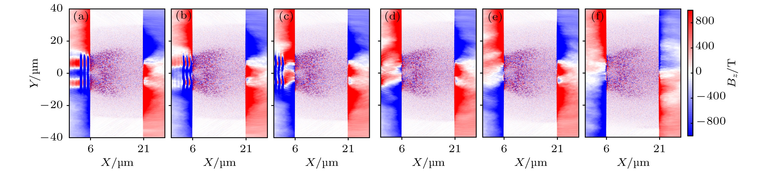图 6 磁场B_z在(a) t = 370, (b) t = 380, (c) t = 390, (d) t = 400, (e) t = 410和(f) t = 460 fs的图像
Figure6. Figure of magnetic field B_z at (a) t = 370, (b) t = 380, (c) t = 390, (d) t = 400, (e) t = 410 and (f) t = 460 fs.

下面结合电子和离子的能谱图, 可以对前面的分析结论进行验证. 图7给出了不同时刻靶后离子和电子的能谱曲线, 能谱和前面图2中靶后鞘场取的是同一个位置区域内的数据, 即两束激光靶后重联区域和单束激光靶后对应于重联区域的范围. 为了能够对比两个算例中的能谱, 作图时单束激光的能谱粒子数在初始统计到的数据上增加了一倍. 观察电子能谱随时间的变化可以发现, 对于高能端(> 0.1 MeV)的电子能谱曲线, 单束激光的靶后电子能谱都要略低于两束激光的, 到后期则明显低于两束激光的电子能谱. 在前面的分析中, 两倍的单束激光靶后鞘场最大值比两束激光靶后重联电场最大值要大. 结合两个模拟中的靶后电子能谱曲线的对比, 认为单束激光的靶后鞘场对电子加速有一定的抑制作用. 图7中靶后的离子能谱则出现了和电子能谱相反的现象, 单束激光的离子能谱比两束激光靶后离子能谱整体都要略高一点, 说明靶后鞘场对离子加速起到了加强的效果. 这也说明靶后鞘场对离子的加速贡献更大, 而重联电场则对离子的加速起到了减弱的作用. 由此可见重联电场会减弱靶后的鞘场, 进而影响离子在靶后的空间分布, 这也就直接导致了单束激光和两束激光在靶后电势分布上不同的结构特点. 上述对于靶后能谱的分析解释了图2中两倍单束激光的靶后鞘场比两束激光的靶后鞘场要大, 磁重联一定程度上减弱了靶后鞘场.
图 7 靶后电子和离子的能谱, 统计选取的粒子及时间分别为(a) 电子300 fs、(b) 离子300 fs、(c) 电子400 fs、(d) 离子400 fs、(e) 电子500 fs和(f) 离子500 fs
Figure7. Electric and ionic energy spectra at (a) 300 fs (electron), (b) 300 fs (ion), (c) 400 fs (electron), (d) 400 fs (ion), (e) 500 fs (electron) and (f) 500 fs (ion).

上面分析了靶后电势分布和磁重联间的联系, 认为通过靶后的电势分布可以判断磁重联的发生. 模拟结果表明单束激光靶后电势呈现双峰结构和实验结果是一致的, 两束激光的情况下靶后电势呈现三峰结构. 分析发现这是受靶前的磁重联影响形成的, 因此认为通过靶后的电势分布可以判断磁重联的发生. 这个结论可以通过超短超强激光驱动磁重联的实验来验证, 记录实验中靶后RCF的成像结果, 成像结果理论上会存在两个并列的环状结构. 值得注意的是, 影响电势分布的因素较多, 而且电势对很多参数细微的变化都非常敏感, 例如靶的几何尺度、靶的材料、激光脉宽、焦斑间距等, 这些则需要更多的实验进行研究.

本文对短脉冲激光和固体平面靶的相互作用进行了二维的PIC数值模拟, 分别模拟了单束激光和两束激光作用在固体平面靶上的物理过程. 通过分析靶后电势分布的特征和磁重联之间的联系, 发现单束激光和双束激光两种情况下靶后的电势分布结构存在显著区别. 单束激光下的靶后电势分布为双峰结构, 这和实验上的结论是一致的. 两束激光下的靶后电势分布呈三峰值结构, 模拟结果证实了这一结论, 但仍需通过实验进一步验证.
感谢北京师范大学超算中心以及国家超级计算广州中心(天河Ⅱ)对本研究工作的支持.