摘要:以永磁铁构成的常规非线性多稳态悬臂梁系统, 若要增加稳态数目, 通常需引入更多的磁铁, 易使系统结构变复杂和参数增多. 本文利用矩形磁铁和环形磁铁的作用, 提出了一种双磁铁构成的多稳态悬臂梁系统. 通过矩形磁铁和环形磁铁之间磁力以及系统势函数的理论分析与实验检验, 证明这种双磁铁悬臂梁系统在不同的磁铁尺寸或磁铁间距下, 可以具有单稳、双稳、三稳和四稳的非线性特征, 为实现由永磁铁构成多稳态悬臂梁系统, 提供了有效简化的设计途径.
关键词: 双磁铁/
多稳态悬臂梁/
磁力/
势函数

English Abstract

全文HTML

--> --> -->

多稳态结构是一种可变形结构, 在外界激励下可产生较大的变形, 变形后的形状无需持续输入能量就可以保持稳定, 并且不同稳态构型之间可以发生相互的跳变^[1-3]. 多稳态结构具有优越的非线性特征, 在很多领域得到广泛的应用^[4-6].
悬臂梁结构是一种可实现多稳态特征的常见结构, 这是因为: 悬臂梁加工简单、刚度低、灵敏度高^[7,8], 在较小激励力下就可发生较大的变形; 在悬臂梁自由端粘贴一块磁铁, 并在与其相对的外部支撑部件上粘贴一块或多块磁铁, 利用磁铁间的相互作用, 就可构造出不同类型的多稳态结构, 比如双稳态、三稳态、四稳态等结构; 悬臂梁及其自由端的磁铁一般可以简化为等效的质量-弹簧-阻尼力学模型^[9], 方便系统的势函数及动力学分析.
多稳态悬臂梁结构常见于振动能量收集系统中, 且以双稳态梁^[10-12]和三稳态梁^[13-15]的结构形式为主. 陈仲生和杨拥民^[10]研究了外加磁力的双稳悬臂梁压电振子的振动特征, 从随机共振角度解释了双稳悬臂梁优于传统线性悬臂梁, 具有宽频的振动响应特性的原因; Podder等^[11]在研究双稳梁电磁振动能量收集中, 通过调整两磁铁的间距优化了系统的频率响应, 并用数值法分析了中、低加速度激励下势阱深度对能量收集的影响; Gao等^[12]通过外部磁铁的弹性支撑设计, 研究了弹性支撑双稳悬臂梁的压电振动能量收集方式, 发现弹性支撑能量收集系统不需要实时调整磁铁间距, 就能够很好地迎合强度时刻变化的随机激励源. Leng等^[13]研究了三稳悬臂梁的压电振动能量收集方式, 得到了在0—120 Hz的随机激励下其发电效果优于双稳悬臂梁压电振动能量收集方式的结果; Zhou等^[14]通过改变三稳悬臂梁中外部磁铁的摆放角度, 研究了一种倒挂式的压电振动能量采集器, 准确得到了系统的非线性刚度和跳跃频率; Deng和Wang^[15]把三稳悬臂梁电磁振动能量收集器的外部磁铁沿圆弧摆放, 研究了不同结构参数对系统输出功率的影响.
在上述利用双稳或三稳悬臂梁结构研究振动能量收集中, 一个显然存在的问题是: 如果系统需要引入更多的非线性稳态数量, 那么需要的磁铁数量也会相应增加, 其结果是可调节的参数不断增多, 这增大了结构的复杂性和系统动力学分析的繁琐性, 不利于系统结构的优化设计.
为了解决多稳态悬臂梁的这一问题, 本文提出双磁铁实现多稳态悬臂梁的构型, 仅利用两个磁铁的相互作用, 通过改变其中一个磁铁的尺寸, 在不同磁铁间距下, 即可实现单稳态、双稳态、三稳态、四稳态特征. 这种双磁铁多稳态悬臂梁构型, 将大大简化系统设计、动力学分析、调试安装等方面的复杂性, 为诸如多稳态悬臂梁结构的振动能量收集系统的设计应用, 提供新的思路和技术方法.

双磁铁多稳态悬臂梁结构由矩形磁铁A、环形磁铁B、悬臂梁C和基座D组成, 如图1所示. 悬臂梁固定在基座上, 矩形磁铁粘贴于悬臂梁的自由端, 环形磁铁与矩形磁铁同极相对并固定在基座上. 不考虑重力的作用, 矩形磁铁与环形磁铁水平对中且相互排斥, 由此形成非线性磁作用力. 当基座受到振动激励后, 矩形磁铁会随着悬臂梁上下振动, 而环形磁铁与基座保持相对静止. 对于不同的结构参数, 这种双磁铁多稳态悬臂梁结构不仅可以表现出单稳态和双稳态特征, 而且还能表现出图1(a)的三稳态和图1(b)的四稳态特征, 也就是说当系统受到合适的外界激励力时, 通过调节结构参数, 悬臂梁可以在图1中的3个或4个势阱之间进行来回的跃迁振荡.
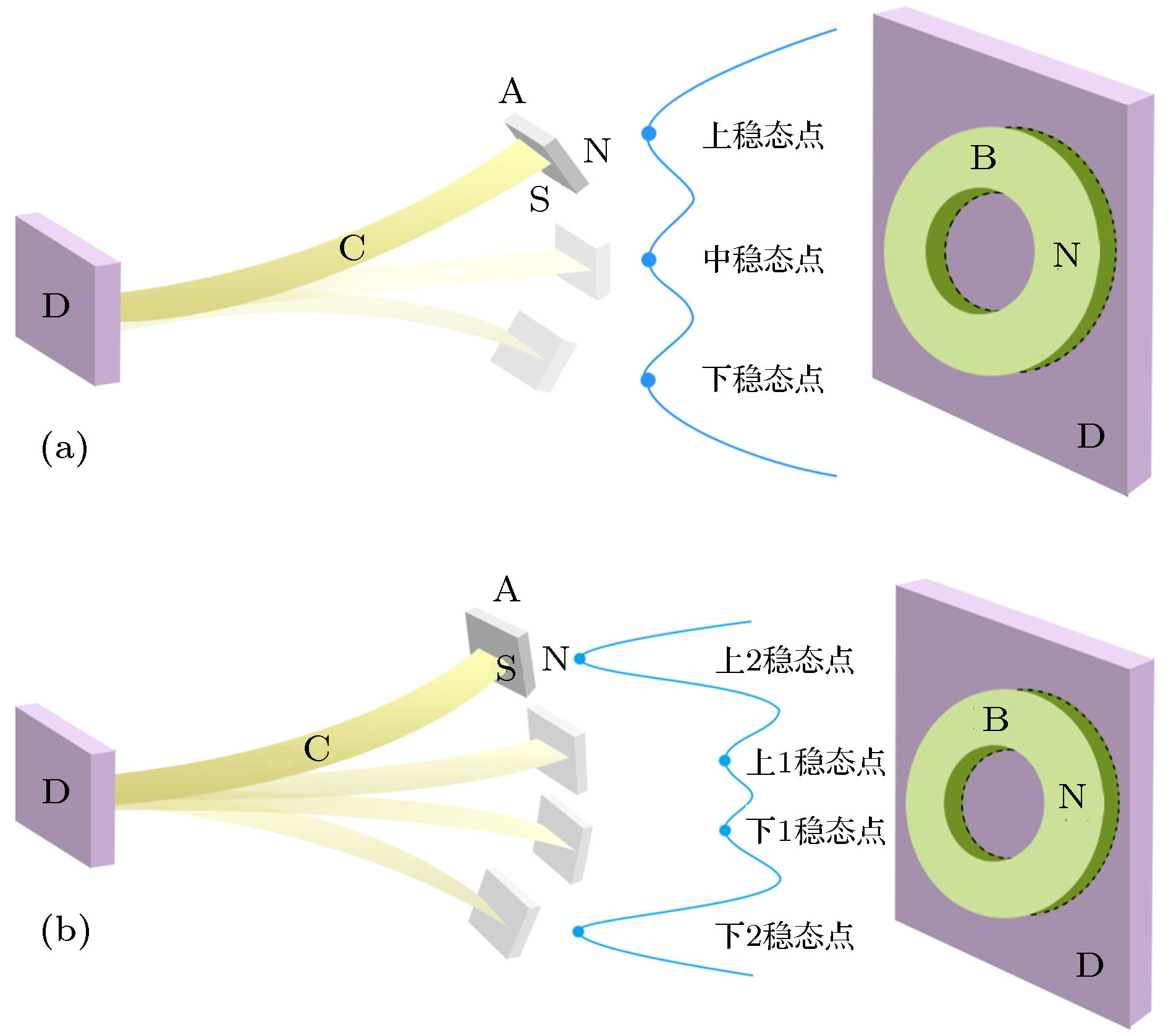图 1 双磁铁多稳态悬臂梁　(a) 三稳状态; (b) 四稳状态
Figure1. Multi-stable cantilever beam with two magnets: (a) The state concluding three stable points; (b) the state concluding four stable points.

对于该双磁铁多稳态悬臂梁系统, 根据牛顿第二定律, 其动力学方程为:

${P_{\rm{A}}} + {F_{\rm{i}}} = {M_{{\rm{eq}}}}{\ddot x_{\rm{A}} } + {\eta _{{\rm{eq}}}}{\dot x_{\rm{A}}} + {K_{{\rm{eq}}}}{x_{\rm{A}}}, $

其中, P_A为外界激励力, F_i为矩形磁铁与环形磁铁之间竖直方向上的磁铁力, x_A为矩形磁铁的竖直位移, M_eq, K_eq, ${\eta _{{\rm{eq}}}}$分别代表系统的等效质量、等效刚度、等效阻尼, 其可由 (2)式—(4)式 计算得出^[16-18]:

${M_{{\rm{eq}}}} = {m_{\rm{A}}} + 33{m_{\rm{C}}}/140, $

${K_{{\rm{eq}}}} = 3{E_{\rm{C}}}{I_{\rm{C}}}/{l_{\rm{C}}}^3, $

${\eta _{{\rm{eq}}}} = {\rm{2}}{M_{{\rm{eq}}}}{\xi _{\rm{r}}}{\omega _{\rm{r}}}, $

(2)式中m_A, m_C分别为矩形磁铁和悬臂梁的质量, (3)式中E_C, I_C, l_C分别为悬臂梁的弹性模量、惯性矩、长度, (4)式中${\xi _{\rm{r}}}$为机械阻尼比、${\omega _{\rm{r}}}$是该等效模型的固有频率.
m_A, m_C, I_C, ${\omega _{\rm{r}}}$的求法如(5)式—(8)式:

${m_{\rm{A}}} = {\rho _{\rm{A}}}{l_{\rm{A}}}{w_{\rm{A}}}{t_{\rm{A}}}, $

${m_{\rm{C}}} = {\rho _{\rm{C}}}{l_{\rm C}}{w_{\rm{C}}}{t_{\rm{C}}}, $

${I_{\rm{C}}} = {w_{\rm{C}}}{t_{\rm{C}}}^3/12, $

${\omega _{\rm{r}}} = \sqrt {{K_{{\rm{eq}}}}/{M_{{\rm{eq}}}}}, $

(5)式中${\rho _{\rm{A}}}$, l_A, w_A, t_A分别为矩形磁铁的密度、长度、宽度、厚度, 本文中用到的矩形磁铁长度和宽度均相等, 即l_A = w_A, (6)式中${\rho _{\rm{C}}}, l_{\rm{C}}, w_{\rm{C}}, t_{\rm{C}}$分别为悬臂梁的密度、长度、宽度、厚度.
为了分析系统的多稳态特征, 首先需要计算两磁铁间的磁力, 然后对不同结构参数的系统进行势函数分析并进行实验验证, 最后在一定结构参数条件下对系统进行随机激励的动力学响应分析.

磁铁间相互作用的磁力分析方法主要有磁偶极子法和磁化电流法两种, 由于磁偶极子法在磁铁间距较小时其磁力分析计算会产生较大的误差^[13], 而磁化电流法对任意磁铁间距的磁力计算精度都比较高, 因此本文选取磁化电流法分析计算双磁铁多稳态悬臂梁结构的非线性磁力.
磁化电流法的基本理论认为^[19,20]: 磁铁周围之所以存在磁场, 是因为被均匀磁化的铁磁体材料内部和表面存在分子电流, 且由于材料内部两相邻电流环的方向相反、相互抵消, 因此其内部电流总和为0, 相当于只有材料表面存在分子电流. 两块磁铁间的相互磁作用力可以视为一个磁铁的表面磁化电流在由另一个磁铁的表面磁化电流产生的磁场中所受的安培力. 所以, 可以把图1中环形磁铁和矩形磁铁之间的磁力计算分为三个步骤: 1)求解环形磁铁表面磁化电流在空间任一点产生的磁感应强度; 2)根据悬臂梁自由端的位移确定矩形磁铁表面磁化电流在空间中的位置; 3)计算二者之间的安培力(即磁力).
2

-->

3.1.环形磁铁在空间中任一点的磁感应强度

根据磁化电流基本理论可知, 环形磁铁内环曲面和外环曲面的磁化电流方向相反, 于是环形磁铁产生的磁场空间中的任一点的磁感应强度, 可看成是内外两个环电流在空间任一点的磁感应强度之矢量和. 由于环形磁铁的内环电流和外环电流都是圆形电流, 因此可任选一圆形实心磁铁, 计算其空间中任一点的磁感应强度.
磁铁表面磁化电流面密度可表示为^[21,22]:

${{K}} = {{M}} \times {\hat { n}}, $

其中, ${{M}}$为磁化强度, 其值为常数, ${\hat { n}}$为磁铁表面的法向单位矢量.
对于一个如图2所示的圆形实心磁铁, 设其磁化强度为${{{M}}_{\rm{B}}}$、厚度为${t_{\rm{B}}}$、半径为${R_{\rm{1}}}$, 根据(9)式, 可以得到其表面磁化电流面密度:
图 2 空间坐标系及圆形实心磁铁的磁化电流示意图
Figure2. Schematic diagram of there-dimension coordinate system and magnetizing currents on the surface of the circular magnet.

${{{K}}_{\rm{B}}} = \left\{ \begin{aligned}& 0, \quad\quad\quad\;\; \left( {\text{左表面}} \right),\\ & 0, \quad\quad \quad\;\;\left( {\text{右表面}} \right),\\ & {M_{\rm{B}}}{\tilde { n}},\quad\quad \left( {\text{曲面}} \right),\end{aligned} \right.$

其中, ${\tilde{ n}} $代表圆形实心磁铁曲面的切线单位矢量. (10)式表示, 圆形实心磁铁的左右表面无磁化电流, 曲面上的表面磁化电流面密度大小为${M_{\rm{B}}}$, 磁化电流方向为逆时针方向(向y轴负方向看).
根据毕奥-萨伐尔(Biot-Savart)定律, 磁铁表面磁化电流中的一个微小电流元$I{\rm{d}}{{l}}$在空间任一点P处产生的磁感应强度${\rm{d}}{{B}}$为:

${\rm{d}}{{B}} = \frac{{{\mu _0}I}}{{4{\text{π}}}}\frac{{{\rm{d}}{{l}} \times {{r}}}}{{{r^3}}}, $

其中, μ₀为真空磁导率, 其值见表1, I 为源电流, ${\rm{d}}{{l}}$是源电流的微小线元素, ${{r}}$为电流元$I{\rm{d}}{{l}}$到空间中任一点P的矢量. 于是整条电流 I 在空间中任一点P处产生的磁感应强度 B 为:

材料	参数	数值
悬臂梁材料: 矽钢	弹性模量EC/GPa	200
	密度ρC/kg·m–3	7700
	长度lC/mm	60
	宽度wC/mm	10
	厚度tC/mm	0.15
矩形磁铁材料: Nd2Fe14B (牌号N35)	密度ρA/kg·m–3	7500
	长度lA/mm	10
	宽度wA/mm	10
	厚度tA/mm	3
	磁化强度MA/A·m–1	6 × 105
环形磁铁材料: Nd2Fe14B (牌号N35)	密度ρB/kg·m–3	7500
	厚度tB/mm	3
	外环直径φ1/mm	40
	内环直径φ2/mm	20
	磁化强度MB/A·m–1	6 × 105
	真空磁导率μ0/N·A–2	4π × 10–7

表1悬臂梁、矩形磁铁、环形磁铁的材料和参数
Table1.Materials and parameters of cantilever beam, rectangular magnet, and ring magnet.

${{B}} = \int\nolimits_L {\frac{{{\mu _0}I}}{{4{\text{π}}}}} \frac{{{\rm{d}}{{l}} \times {{r}}}}{{{r^3}}}, $

其中, $L$为电流积分路径.
对于图2所示的坐标系中的圆形实心磁铁, 取I为距xz平面为$l$的任一条电流, 在I上任选一段电流元$I{\rm{d}}{{l}}$, 则该电流元在空间中的坐标为$\left( {{R_1}\sin \theta, l, {R_1}\cos \theta } \right)$, 于是坐标原点到电流元$I{\rm{d}}{{l}}$的矢量为${{l}} = {R_1}\sin \theta {{i}} + l{{j}} + {R_1}\cos \theta {{k}}$, 其中${{i}}$, ${{j}}$, ${{k}}$分别为x, y, z方向上的单位矢量, 所以${\rm{d}}{{l}} = {R_1}\cos \theta {\rm{d}}\theta {{i}} + 0{{j}} + ( - {R_1}\sin \theta {\rm{d}}\theta ){{k}}$, ${\rm{d}}{{l}}$到空间中任一点$P(x, y, z)$的矢量${{r}} = (x - {R_1}\sin \theta ){{i}} + (y - l){{j}} + (z - {R_1}\cos \theta ){{k}}$.
因此, ${\rm{d}}{{l}} \!\times\! {{r}} \!=\! (y - l){R_1}\sin \theta {\rm{d}}\theta {{i}} \!+\! {R_1}({R_1} \!-\! x\sin \theta - z\cos \theta ){\rm{d}}\theta {{j}} +(y - l){R_1}\cos \theta {{k}}$, 将其代入(12)式, 得到圆形实心磁铁磁化电流在图2空间坐标系中任一点$P(x, y, z)$处的磁感应强度:

$\begin{split} {{{B}}_1}(x,y,z) =\;& {B_{1i}}(x,y,z){{i}} + {B_{1j}}(x,y,z){{j}} + {B_{1k}}(x,y,z){{k}} \\ = \;& \frac{{{\mu _0}{M_{\rm{B}}}}}{{4{\text{π}}}}\int\nolimits_{\textstyle - \frac{{{t_{\rm{B}}}}}{2}}^{\textstyle\frac{{{t_{\rm{B}}}}}{2}} {{\rm{d}}l\int\nolimits_0^{2{\text{π}}} {\frac{{(y - l){R_1}\sin \theta }}{{{{\left[ {{{(x - {R_1}\sin \theta )}^2} + {{(y - l)}^2} + {{(z - {R_1}\cos \theta )}^2}} \right]}^{\frac{3}{2}}}}}} } {\rm{d}}\theta {{i}} \\ & + \frac{{{\mu _0}{M_{\rm{B}}}}}{{4{\text{π}}}}\int\nolimits_{\textstyle - \frac{{{t_{\rm{B}}}}}{2}}^{\textstyle\frac{{{t_{\rm{B}}}}}{2}} {{\rm{d}}l\int\nolimits_0^{2{\text{π}}} {\frac{{{R_1}({R_1} - x\sin \theta - z\cos \theta )}}{{{{\left[ {{{(x - {R_1}\sin \theta )}^2} + {{(y - l)}^2} + {{(z - {R_1}\cos \theta )}^2}} \right]}^{\frac{3}{2}}}}}} } {\rm{d}}\theta {{j}} \\ &+ \frac{{{\mu _0}{M_{\rm{B}}}}}{{4{\text{π}}}}\int\nolimits_{\textstyle - \frac{{{t_{\rm{B}}}}}{2}}^{\textstyle\frac{{{t_{\rm{B}}}}}{2}} {{\rm{d}}l\int\nolimits_0^{2{\text{π}}} {\frac{{(y - l){R_1}\cos \theta }}{{{{\left[ {{{(x - {R_1}\sin \theta )}^2} + {{(y - l)}^2} + {{(z - {R_1}\cos \theta )}^2}} \right]}^{\frac{3}{2}}}}}} } {\rm{d}}\theta {{k}}.\end{split} $

设环形磁铁磁化强度也为${{{M}}_{\rm{B}}}$、厚度也为${t_{\rm{B}}}$、外环半径也为${R_{\rm{1}}}$、内环半径为${R_{\rm{2}}}$, 则其外环表面磁化电流在图2空间坐标系中任一点$P(x, y, z)$处的磁感应强度也如(13)式. 因为内环表面磁化电流与外环表面磁化电流方向相反, 所以内环表面磁化电流在图2空间坐标系中任一点$P(x, y, z)$处的磁感应强度为:

$\begin{split} {{{B}}_{\rm{2}}}(x,y,z) =\; & {B_{{\rm{2}}i}}(x,y,z){{i}} + {B_{{\rm{2}}j}}(x,y,z){{j}} + {B_{{\rm{2}}k}}(x,y,z){{k}} \\ = \;& - \frac{{{\mu _0}{M_{\rm{B}}}}}{{4{\text{π}}}}\int\nolimits_{\textstyle - \frac{{{t_{\rm{B}}}}}{2}}^{\textstyle\frac{{{t_{\rm{B}}}}}{2}} {{\rm{d}}l\int\nolimits_0^{2{\text{π}}} {\frac{{(y - l){R_{\rm{2}}}\sin \theta }}{{{{\left[ {{{(x - {R_{\rm{2}}}\sin \theta )}^2} + {{(y - l)}^2} + {{(z - {R_{\rm{2}}}\cos \theta )}^2}} \right]}^{\frac{3}{2}}}}}} } {\rm{d}}\theta {{i}} \\ & -\frac{{{\mu _0}{M_{\rm{B}}}}}{{4{\text{π}}}}\int\nolimits_{ \textstyle- \frac{{{t_{\rm{B}}}}}{2}}^{\textstyle\frac{{{t_{\rm{B}}}}}{2}} {{\rm{d}}l\int\nolimits_0^{2{\text{π}}} {\frac{{{R_{\rm{2}}}({R_{\rm{2}}} - x\sin \theta - z\cos \theta )}}{{{{\left[ {{{(x - {R_{\rm{2}}}\sin \theta )}^2} + {{(y - l)}^2} + {{(z - {R_{\rm{2}}}\cos \theta )}^2}} \right]}^{\frac{3}{2}}}}}} } {\rm{d}}\theta {{j}} \\ & - \frac{{{\mu _0}{M_{\rm{B}}}}}{{4{\text{π}}}}\int\nolimits_{ \textstyle- \frac{{{t_{\rm{B}}}}}{2}}^{\textstyle\frac{{{t_{\rm{B}}}}}{2}} {{\rm{d}}l\int\nolimits_0^{2{\text{π}}} {\frac{{(y - l){R_{\rm{2}}}\cos \theta }}{{{{\left[ {{{(x - {R_{\rm{2}}}\sin \theta )}^2} + {{(y - l)}^2} + {{(z - {R_{\rm{2}}}\cos \theta )}^2}} \right]}^{\textstyle\frac{3}{2}}}}}} } {\rm{d}}\theta {{k}}. \end{split} $

对(13)式和(14)式进行矢量叠加, 便可以得到环形磁铁在图2所示的空间坐标系中任一点$P(x, y, z)$处的总磁感应强度为:

$\small\begin{split} &{{B}}(x,y,z) ={{{B}}_1}(x,y,z) + {{{B}}_{\rm{2}}}(x,y,z)={B_i}(x,y,z){{i}} + {B_j}(x,y,z){{j}} + {B_k}(x,y,z){{k}} = \\ \; &\left[ {{B_{1i}}(x,y,z) + {B_{{\rm{2}}i}}(x,y,z)} \right]{{i}} + \left[ {{B_{1j}}(x,y,z) + {B_{{\rm{2}}j}}(x,y,z)} \right]{{j}} + \left[ {{B_{1k}}(x,y,z) + {B_{{\rm{2}}k}}(x,y,z)} \right]{{k}} = \\ \; & \frac{{{\mu _0}{M_{\rm{B}}}}}{{4{\text{π}}}}\int\nolimits_{\textstyle - \frac{{{t_{\rm{B}}}}}{2}}^{\textstyle\frac{{{t_{\rm{B}}}}}{2}} {{\rm{d}}l\int\nolimits_0^{2{\text{π}}} {\left\{ {\frac{{(y - l){R_1}\sin \theta }}{{{{\left[ {{{(x \!-\! {R_1}\sin \theta )}^2} \!+\! {{(y \!-\! l)}^2} \!+\! {{(z \!-\! {R_1}\cos \theta )}^2}} \right]}^{\textstyle\frac{3}{2}}}}} \!-\! \frac{{(y \!-\! l){R_2}\sin \theta }}{{{{\left[ {{{(x \!-\! {R_2}\sin \theta )}^2} \!+\! {{(y \!-\! l)}^2} \!+\! {{(z \!-\! {R_2}\cos \theta )}^2}} \right]}^{\textstyle\frac{3}{2}}}}}} \right\}} } {\rm{d}}\theta {{i}} \\&+\! \frac{{{\mu _0}{M_{\rm{B}}}}}{{4{\text{π}}}}\int\nolimits_{ \textstyle- \frac{{{t_{\rm{B}}}}}{2}}^{\textstyle\frac{{{t_{\rm{B}}}}}{2}} {{\rm{d}}l\int\nolimits_0^{2{\text{π}}} {\left\{ {\frac{{{R_1}({R_1} \!-\! x\sin \theta \!-\! z\cos \theta )}}{{{{\left[ {{{(x \!-\! {R_1}\sin \theta )}^2} \!+\! {{(y \!-\! l)}^2} \!+\! {{(z \!-\! {R_1}\cos \theta )}^2}} \right]}^{\textstyle\frac{3}{2}}}}} \!-\! \frac{{{R_2}({R_2} \!-\! x\sin \theta \!-\! z\cos \theta )}}{{{{\left[ {{{(x \!-\! {R_2}\sin \theta )}^2} \!+\! {{(y \!-\! l)}^2} \!+\! {{(z \!-\! {R_2}\cos \theta )}^2}} \right]}^{\textstyle\frac{3}{2}}}}}} \right\}} } {\rm{d}}\theta {{j}} \\& +\!\frac{{{\mu _0}{M_{\rm{B}}}}}{{4{\text{π}}}}\int\nolimits_{\textstyle - \frac{{{t_{\rm{B}}}}}{2}}^{\textstyle\frac{{{t_{\rm{B}}}}}{2}} {{\rm{d}}l\int\nolimits_0^{2{\text{π}}} {\left\{ {\frac{{(y - l){R_1}\cos \theta }}{{{{\left[ {{{(x \!-\! {R_1}\sin \theta )}^2} \!+\! {{(y \!-\! l)}^2} \!+\! {{(z \!-\! {R_1}\cos \theta )}^2}} \right]}^{\textstyle\frac{3}{2}}}}} \!-\! \frac{{(y \!-\! l){R_2}\cos \theta }}{{{{\left[ {{{(x \!-\! {R_2}\sin \theta )}^2} + {{(y \!-\! l)}^2} \!+\! {{(z \!-\! {R_2}\cos \theta )}^2}} \right]}^{\textstyle\frac{3}{2}}}}}} \right\}} } {\rm{d}}\theta {{k}} .\end{split}\normalsize$

为了验证(15)式的正确性, 在图2空间坐标系的xy平面中任取y = 6.0 mm和y = 10.0 mm两个值, 并根据表1环形磁铁的参数, 对(15)式进行数值分析, 得到磁感应强度${B_i}$和${B_j}$随$x$的变化关系, 如图3中的蓝色实曲线. 选取表2中的高斯计等仪器搭建图4所示的磁感应强度测量系统, 在对应的数值模拟坐标空间值处测量相应的磁感应强度, 得到${B_i}$和${B_j}$随$x$的变化关系, 如图3中的红色星号点曲线. 比较图3中仿真曲线和实验数据可以看出, 二者结果吻合很好, 验证了(15)式的正确性.

实验器材	型号
高斯计	BST100
推拉式测力计	HF-5
激光位移传感器	LK-G5001V

表2实验器材及其型号
Table2.Experimental equipments and models.

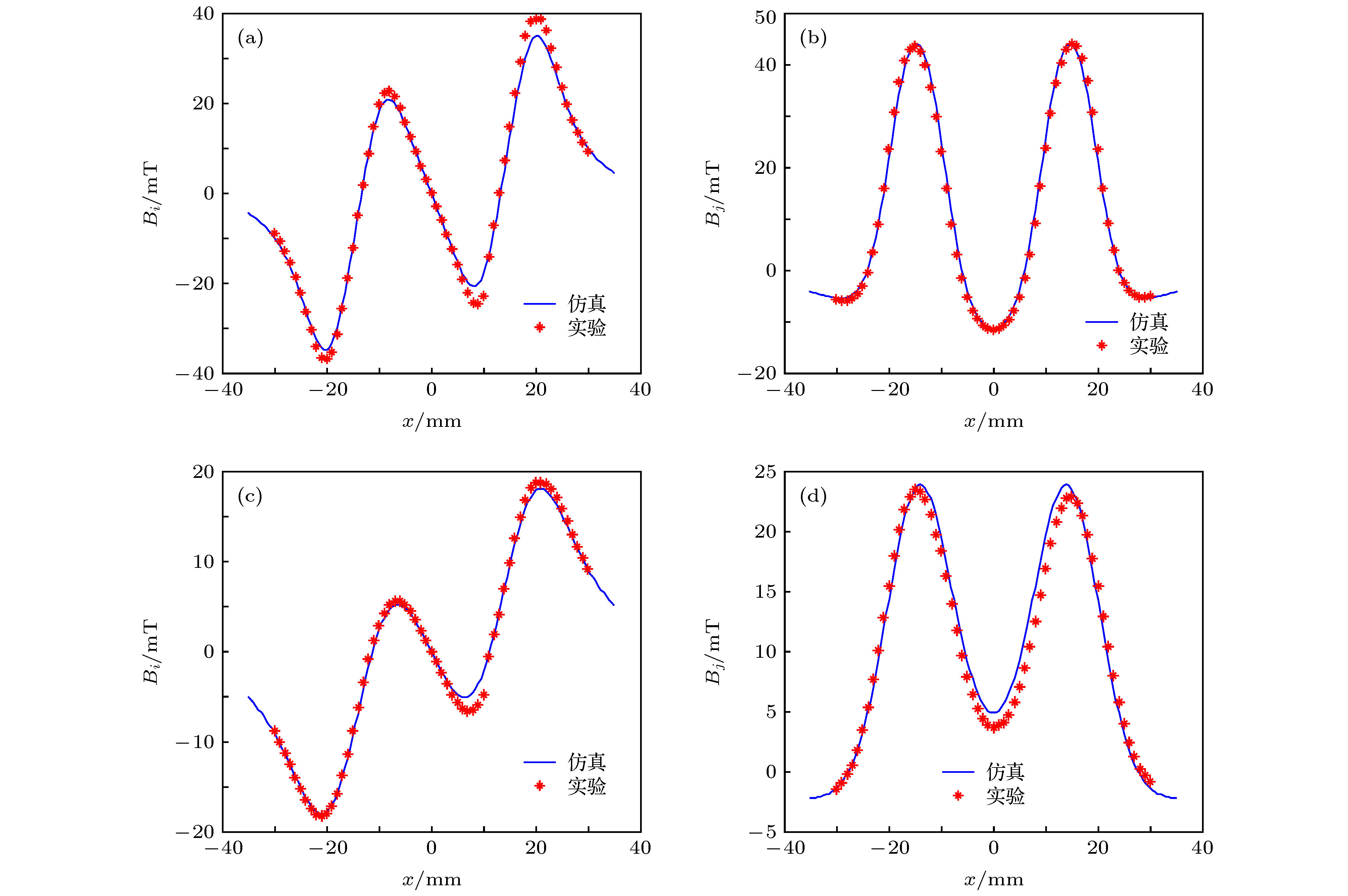图 3 磁感应强度B_i, B_j随x的变化关系　(a) B_i随x的变化, y = 6.0 mm; (b) B_j随x的变化, y = 6.0 mm; (c) B_i随x的变化, y = 10.0 mm; (d) B_j随x的变化, y = 10.0 mm
Figure3. The curves of B_i and B_j varying with x: (a) The curves of B_i varying with x, y = 6.0 mm; (b) the curves of B_j varying with x, y = 6.0 mm; (c) the curves of B_i varying with x, y = 10.0 mm; (d) the curves of B_j varying with x, y = 10.0 mm.

图 4 磁感应强度测量系统　(a)B_i测量; (b)B_j测量
Figure4. Magnetic induction intensity measurement system: (a) The measurement of B_i; (b) the measurement of B_j.

2 -->

3.2.矩形磁铁磁化电流在空间中的位置

悬臂梁在振动过程中会发生弯曲, 并使得梁自由端的磁铁发生偏转, 如图5所示, 因此需要准确计算磁铁位置才能确定矩形磁铁磁化电流在空间中的位置.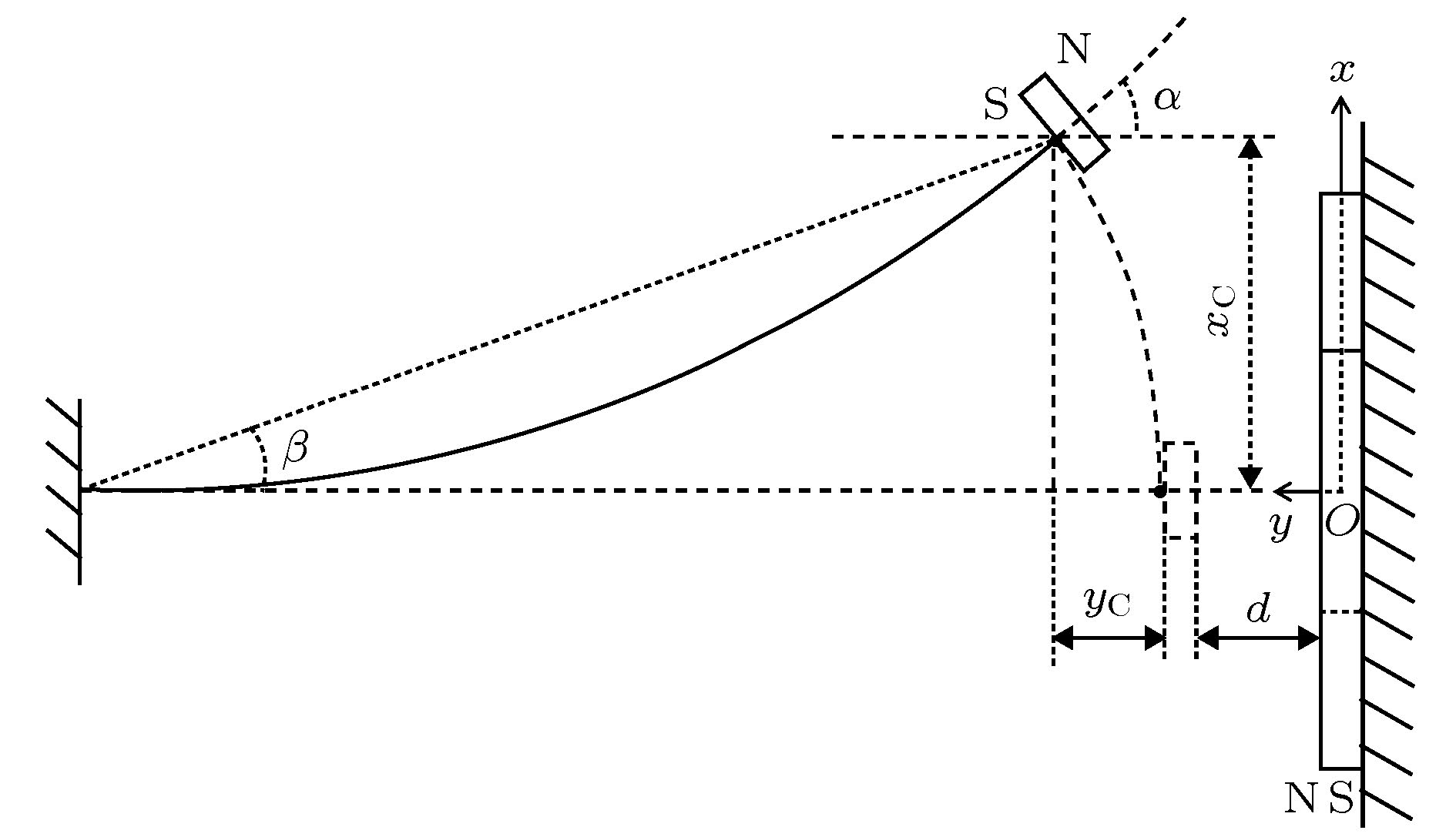
图 5 悬臂梁弯曲状态及其矩形磁铁的坐标位置
Figure5. The position of the rectangular magnet in coordinate system when the cantilever beam is bent.

悬臂梁在弯曲时, 其自由端水平位移y_C与竖直位移x_C的几何关系受梁的长短、厚薄、材料等因素的影响, 现有的经验计算方法有两种, 如(16a)式^[21,22]和(16b)式^[20]:

${y_{\rm{C}}} \approx {l_{\rm{C}}}\Big[ {1 - \sqrt {1 - {{\big( {{{{x_{\rm{C}}}}}/{{{l_{\rm{C}}}}}} \big)}^2}} } \;\Big], \tag{16a}$

${y_{\rm{C}}} \approx {l_{\rm{C}}} - \frac{{{l_{\rm{C}}}}}{{\dfrac{{{{\text{π}} ^2}{x_{\rm{C}}}^2}}{{12{l_{\rm{C}}}^2}} + 1}}.\tag{16b}$

为了比较两种经验计算方法对本文中所选取悬臂梁的适用性, 根据表1中悬臂梁的参数, 对(16a)式和(16b)式进行数值分析, 分别得到${y_{\rm{C}}}$随${x_{\rm{C}}}$的变化关系曲线, 如图6中的黑色实线和青色虚线. 选取表2中的激光位移传感器等仪器搭建图7所示的位移测量系统, 测量出${y_{\rm{C}}}$随${x_{\rm{C}}}$的变化关系曲线, 如图6中的蓝色圆圈点线. 比较图中实验测量结果与(16a)式和(16b)式数值分析结果不难发现, (16b)式得到的仿真曲线更贴近实验数据, 计算更准确, 所以本文选用(16b)式来确定${y_{\rm{C}}}$与${x_{\rm{C}}}$的关系.
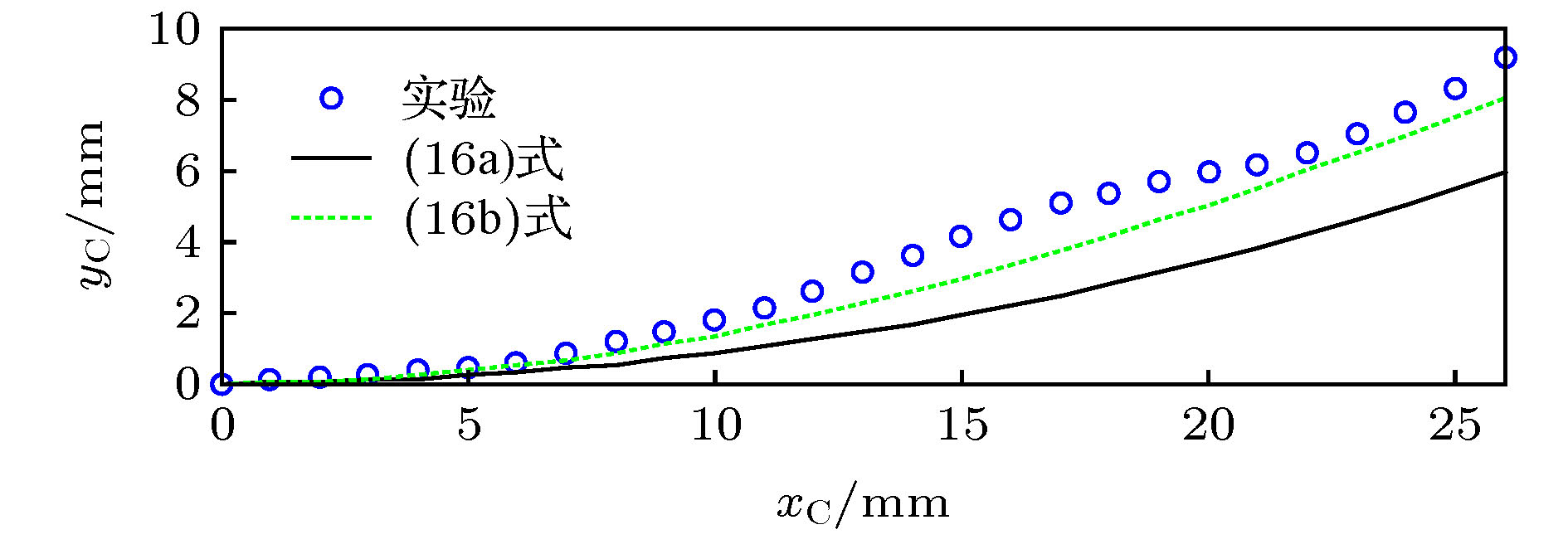图 6 梁自由端磁铁位置的两种计算方法
Figure6. Two kinds of calculation of the position of the magnet at the free end of the beam.

图 7 位移测量系统
Figure7. Displacement measuring device.

对于悬臂梁弯曲时其自由端矩形磁铁的偏转角α, 由经验公式(17)式确定:

$ \sin \alpha \approx {{{x_{\rm{C}}}}}/{{{l_{\rm{C}}}}}.$

当磁化强度为${{{M}}_{\rm{A}}}$的矩形磁铁偏转角为$\alpha $时, 根据(9)式, 其表面磁化电流面密度为:

${{{K}}_A} = \begin{cases}{M_{\rm{A}}}{{k}}, & \left( {\text{上表面}} \right),\\ - {M_{\rm{A}}}{{k}}, & \left( {\text{下表面}} \right),\\0, & \left( {\text{左侧面}} \right),\\0, & \left( {\text{右侧面}} \right),\\ - {M_{\rm{A}}}\cos \alpha {{i}} + ( - {M_{\rm{A}}}\sin \alpha ){{j}}, & \left( {\text{前表面}} \right),\\{M_{\rm{A}}}\cos \alpha {{i}} + {M_A}\sin \alpha {{j}}, & \left( {{\text{后表面}}} \right),\end{cases}$

即矩形磁铁左右表面无磁化电流, 只有上、下、前、后表面存在磁化电流, 如图8所示.
图 8 矩形磁铁尺寸及磁化电流示意图
Figure8. Schematic diagram of the size of the rectangular magnet and the magnetizing currents on the surface of the rectangular magnet.

根据(16b)式和(17)式, 结合图5和图8, 当悬臂梁的自由端竖直位移为${x_{\rm{C}}}$时, 可以求出矩形磁铁体心的空间坐标$\left({x_{\rm{C}}} + \dfrac{{{t_{\rm{A}}}}}{2}\sin \alpha, d + \dfrac{{{t_{\rm{B}}}}}{2} + {t_{\rm{A}}} + {y_{\rm{C}}} - \dfrac{{{t_{\rm{A}}}}}{2}\cos \alpha, 0 \right)$、矩形磁铁上表面磁化电流中心的空间坐标$\left({x_{\rm{C}}} + \dfrac{{{t_{\rm{A}}}}}{2}\sin \alpha {\rm{ + }}\dfrac{{{l_{\rm{A}}}}}{{\rm{2}}}\cos \alpha, d + \dfrac{{{t_{\rm{B}}}}}{2} + {t_{\rm{A}}} + {y_{\rm{C}}} - \dfrac{{{t_{\rm{A}}}}}{2}\cos \alpha + \dfrac{{{l_{\rm{A}}}}}{2}\sin \alpha, 0 \right)$、矩形磁铁下表面磁化电流中心的空间坐标$\left({x_{\rm{C}}} + \dfrac{{{t_{\rm{A}}}}}{2}\sin \alpha - \dfrac{{{l_{\rm{A}}}}}{{\rm{2}}}\cos \alpha, d + \dfrac{{{t_{\rm{B}}}}}{2} + {t_{\rm{A}}} + {y_{\rm{C}}} - \dfrac{{{t_{\rm{A}}}}}{2}\cos \alpha - \dfrac{{{l_{\rm{A}}}}}{2}\sin \alpha, 0 \right)$、矩形磁铁前表面磁化电流中心的空间坐标$\left({x_{\rm{C}}} + \dfrac{{{t_{\rm{A}}}}}{2}\sin \alpha, d + \dfrac{{{t_{\rm{B}}}}}{2} + {t_{\rm{A}}} + {y_{\rm{C}}} - \dfrac{{{t_{\rm{A}}}}}{2}\cos \alpha, \dfrac{{{w_{\rm{A}}}}}{{\rm{2}}}\right)$、矩形磁铁后表面磁化电流中心的空间坐标$\left({x_{\rm{C}}} + \dfrac{{{t_{\rm{A}}}}}{2}\sin \alpha, d + \dfrac{{{t_{\rm{B}}}}}{2} + {t_{\rm{A}}} + {y_{\rm{C}}} - \dfrac{{{t_{\rm{A}}}}}{2}\cos \alpha, - \dfrac{{{w_{\rm{A}}}}}2 \right)$.
2 -->

3.3.矩形磁铁与环形磁铁间的磁力

矩形磁铁表面磁化电流在环形磁铁产生的磁场中所受的安培力可表示为^[21]:

${{F}} = \iint\nolimits_S {{{{K}}_{\rm{A}}}} \times {{B}}{\rm{d}}s, $

将(18)式代入(19)式, 即可得到矩形磁铁所受到的磁力:

$\begin{split}\;& {{F}} = {F_i}{{i}} + {F_j}{{j}} + {F_k}{{k}}= \\ \;&\bigg[ \iint\nolimits_{{S_1}} {( - {M_{\rm{A}}}{B_j}}){\rm{d}}s + \iint\nolimits_{{S_2}} {{M_{\rm{A}}}{B_j}}{\rm{d}}s \\& + \iint\nolimits_{{S_3}} {( - {M_{\rm{A}}}\sin \alpha {B_k}}){\rm{d}}s + \iint\nolimits_{{S_4}} {{M_{\rm{A}}}\sin \alpha {B_k}}{\rm{d}}s \bigg]{{i}} \\& + \bigg[\iint\nolimits_{{S_1}} {{M_{\rm{A}}}{B_i}}{\rm{d}}s + \iint\nolimits_{{S_2}} {( - {M_{\rm{A}}}{B_i})}{\rm{d}}s \\& + \iint\nolimits_{{S_3}} {{M_{\rm{A}}}\cos \alpha {B_k}}{\rm{d}}s + \iint\nolimits_{{S_4}} {( - {M_{\rm{A}}}\cos \alpha {B_k}}){\rm{d}}s \bigg]{{j}} \\& + \bigg[ \iint\nolimits_{{S_3}} {( - {M_{\rm{A}}}\cos \alpha {B_j}}){\rm{d}}s + \iint\nolimits_{{S_3}} {{M_{\rm{A}}}\sin \alpha {B_i}}{\rm{d}}s \\& + \iint\nolimits_{{S_4}} {{M_{\rm{A}}}\cos \alpha {B_j}}{\rm{d}}s + \iint\nolimits_{{S_4}} {( - {M_{\rm{A}}}\sin \alpha {B_i}}){\rm{d}}s \bigg]{{k}},\end{split} $

其中, ${S_1}$, ${S_2}$分别为矩形磁铁上、下表面的面积, ${S_1} = {S_2} = {t_{\rm{A}}}{w_{\rm{A}}}$, ${S_3}$, ${S_4}$分别为矩形磁铁前、后表面的面积, ${S_3} = {S_4} = {t_{\rm{A}}}{l_{\rm{A}}}$, 矩形磁铁尺寸如图8所示.
为了验证(20)式的合理性, 在图5的坐标系中, 任取d = 5.8 mm和d = 8.0 mm两个值, 根据表1中的参数, 对(20)式进行数值仿真, 得到${F_i}$和${F_j}$随${x_{\rm{C}}}$的变化关系曲线, 如图9中的蓝色实线. 选取表2中的推拉式测力计和激光位移传感器等仪器搭建图10所示的磁力测量系统, 在对应的数值模拟坐标空间值处测量相应的磁力, 得到磁力${F_i}$, ${F_j}$随${x_{\rm{C}}}$的变化关系曲线, 如图9中的红色星号点线. 由图9可以看出, 实验数据与仿真数据基本吻合, 验证了(20)式磁力分析模型的合理性. 需要说明的是, 由于实验中选用的测力计的最小输入值为0.05 N, 因此图9中小于0.05 N的磁力只能用零值点表示.
图 9 F_i, F_j随x_C的变化关系　(a) F_i随x_C的变化关系, d = 5.8 mm; (b)F_j随x_C的变化关系, d = 5.8 mm; (c) F_i随x_C的变化关系, d = 8.0 mm; (d) F_j随x_C的变化关系, d = 8.0 mm
Figure9. The curves of F_i and F_j varying with x_C: (a) The curves of F_i varying with x_C, d = 5.8 mm; (b) the curves of F_j varying with x_C, d = 5.8 mm; (c) the curves of F_i varying with x_C, d = 8.0 mm; (d) the curves of F_j varying with x_C, d = 8.0 mm.

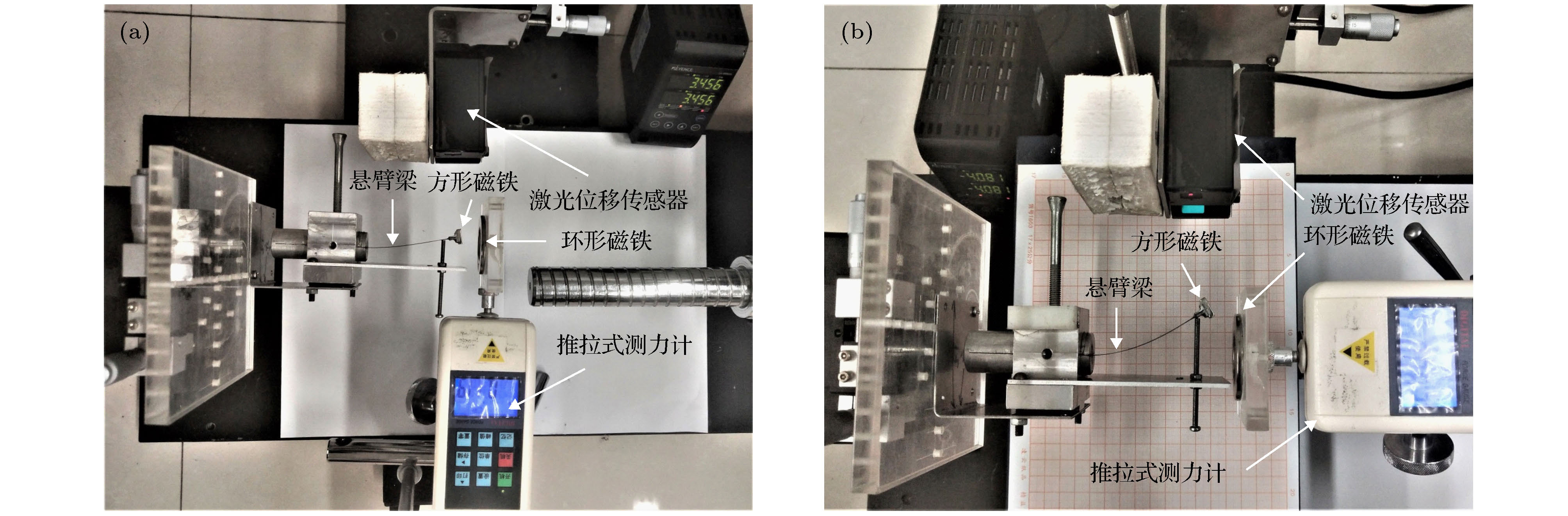图 10 磁力测量系统　(a) F_i 测量; (b) F_j测量
Figure10. Magnetic force measurement system: (a) The measurement of F_i; (b) the measurement of F_j.

对于该双磁铁多稳态悬臂梁系统, 如果定义初始水平位置(${x_{\rm{C}}} = 0$)为系统的零势能点, 且不考虑重力势能, 那么当悬臂梁自由端在竖直方向的位移为${x_{\rm{C}}}$时, 系统总势能$V$包括等效弹性恢复力做的功

${W_1} = \displaystyle\int_0^{{x_{\rm{C}}}} {{K_{{\rm{eq}}}}x} {\rm{d}}x,$

F_i做的功

${W_2} = - \displaystyle\int_0^{{x_{\rm{C}}} +\textstyle \frac{{{t_{\rm{A}}}}}{2}\sin \alpha } {{F_i}} {\rm{d}}x ,$

F_j 做的功

${W_3} = - \displaystyle\int_0^{\textstyle\frac{{{t_{\rm{A}}}}}{{\rm{2}}} + {y_{\rm{C}}}\textstyle - \frac{{{t_{\rm{A}}}}}{2}\cos \alpha } {{F_j}} {\rm{d}}y,$

即

$\begin{split}\; & V = {W_1} + {W_2} + {W_3} = \int_0^{{x_{\rm{C}}}} {{K_{{\rm{eq}}}}x} {\rm{d}}x \\ &- \int_0^{{x_{\rm{C}}} + \frac{{{t_{\rm{A}}}}}{2}\sin \alpha } {{F_i}} {\rm{d}}x - \int_0^{\frac{{{t_{\rm{A}}}}}{{\rm{2}}} + {y_{\rm{C}}} - \frac{{{t_{\rm{A}}}}}{2}\cos \alpha } {{F_j}} {\rm{d}}y,\end{split} $

(21)式便是系统势函数表达式, 就其物理含义而言, 势函数代表的是系统的势能. 所以, (21)式也可称之为系统势能函数. 根据矩形磁铁和环形磁铁的间距及其尺寸等参数, 可以分析双磁铁悬臂梁系统的稳态特性.
2

-->

4.1.系统势函数随磁铁间距的变化

根据表1, 设置矩形磁铁和环形磁铁的尺寸分别为10 mm × 10 mm × 3 mm和40 mm(φ₁) × 20 mm(φ₂) × 3 mm, 对(21)式进行数值分析, 得到图11不同磁铁间距d的系统势函数变化图像.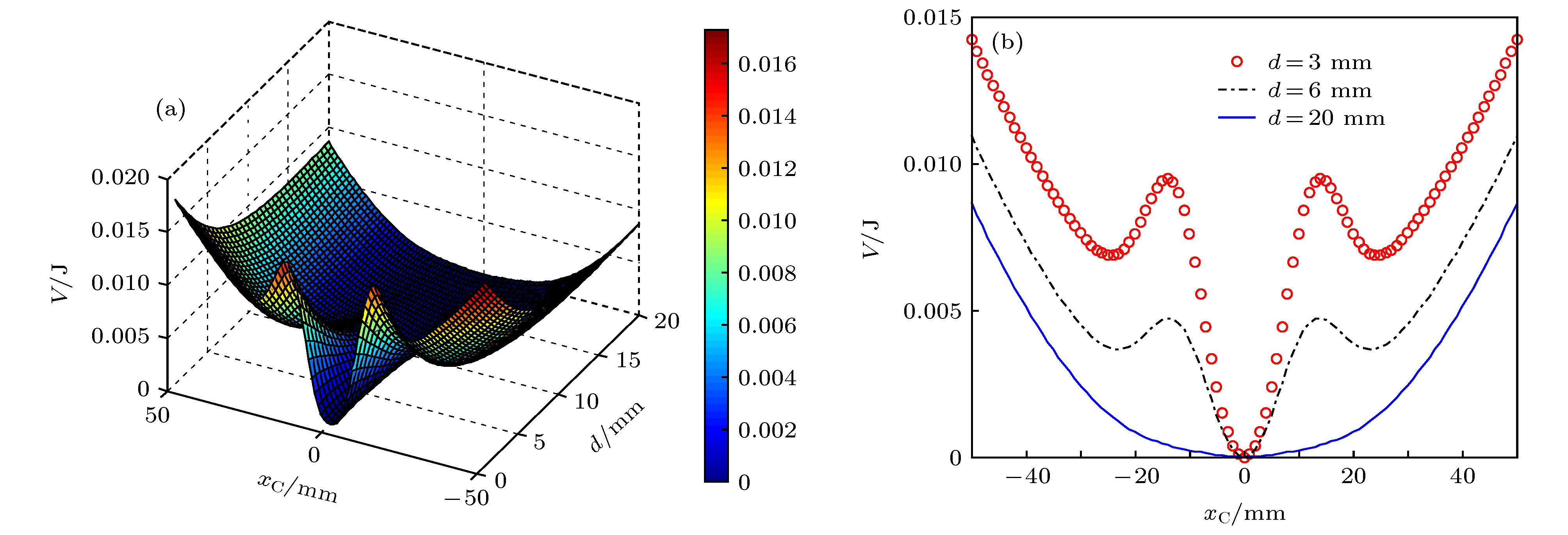
图 11 矩形磁铁(10 mm × 10 mm × 3 mm)与环形磁铁(40 mm (φ₁) × 20 mm (φ₂) × 3 mm)作用的系统势函数　(a)系统势函数三维图; (b)磁铁间距分别为d = 3 mm, d = 6 mm, d = 20 mm时系统势函数二维图
Figure11. The system potential function varying with d when the size of the rectangular magnet is 10 mm × 10 mm × 3 mm and the ring magnet is 40 mm (φ₁) × 20 mm (φ₂) × 3 mm: (a) Three dimensional diagram of system potential function; (b) two dimensional diagram of system potential function when d = 3 mm, d = 6 mm and d = 20 mm.

由图11可知, 随着磁铁间距的增大, 系统势函数从三稳状态逐渐变成单稳状态. 当磁铁间距d很小时, 如d = 3 mm, 系统中间势阱较深, 其两侧势阱相对较浅. 当d增大时, 如d = 6 mm, 系统的三个势阱均会变浅. 如果继续增大磁铁间距, 如d = 20 mm, 则系统的三个势阱几乎消失, 系统退化为一个单稳状态.
保持环形磁铁的尺寸不变, 当增大矩形磁铁尺寸时, 系统势函数随磁铁间距d的增大, 会出现由三稳状态或四稳状态先退化为双稳状态再退化为单稳状态的过程. 以20 mm × 20 mm × 3 mm和30 mm × 30 mm × 3 mm的矩形磁铁为例, 作出系统势函数随磁铁间距d的变化图像, 如图12所示. 可以看到, 当矩形磁铁的尺寸为20 mm × 20 mm × 3 mm时, 随着磁铁间距的增大, 系统势函数依次从三稳状态逐渐变成双稳和单稳状态; 当矩形磁铁的尺寸为30 mm × 30 mm × 3 mm, 随着磁铁间距的增大, 系统势函数依次从四稳状态逐渐变成双稳和单稳状态.
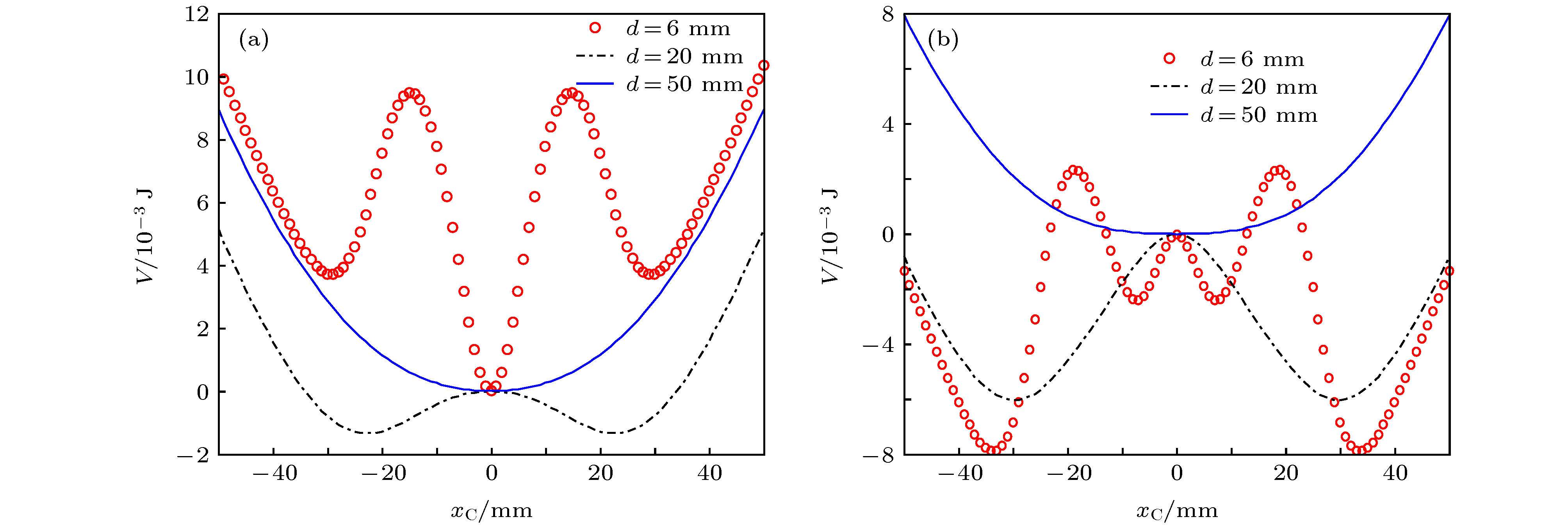图 12 系统势函数随d的变化 　(a)矩形磁铁尺寸为 20 mm × 20 mm × 3 mm; (b) 矩形磁铁尺寸为 30 mm × 30 mm × 3 mm
Figure12. The system potential function varying with d: (a) The size of the rectangular magnet is 20 mm × 20 mm × 3 mm; (b) the size of the rectangular magnet is 30 mm × 30 mm × 3 mm.

2 -->

4.2.系统势函数随磁铁尺寸的变化

取磁铁间距d = 6 mm, 并保持环形磁铁尺寸不变, 令矩形磁铁的长度和宽度相等, 厚度保持3 mm不变, 以矩形磁铁长度l_A为变量, 对(21)式进行数值分析, 得到如图13所示的系统势函数变化图像.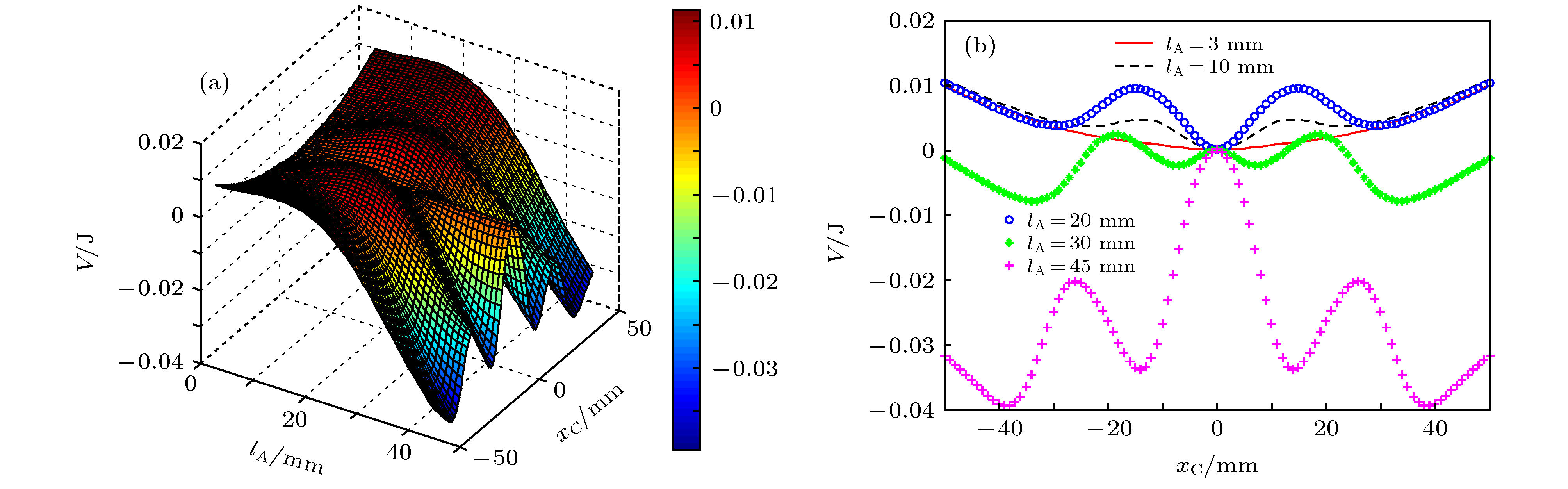
图 13 磁铁间距d = 6 mm, 不同矩形磁铁尺寸与环形磁铁(40 mm(φ₁) × 20 mm(φ₂) × 3 mm)作用的系统势函数　(a) 系统势函数三维图; (b) 矩形磁铁长度分别为l_A = 3 mm, l_A = 10 mm, l_A = 20 mm, l_A = 30 mm, l_A = 45 mm时系统势函数二维图
Figure13. The system potential function varying with l_A when d = 6 mm and the size of the ring magnet is 40 mm(φ₁) × 20 mm(φ₂) × 3 mm: (a) Three dimensional diagram of system potential function; (b) two dimensional diagram of system potential function when l_A = 3 mm, l_A = 10 mm, l_A = 20 mm, l_A = 30 mm and l_A = 45 mm.

从图13可以看出, 随着矩形磁铁长度的增大, 系统势函数从单稳状态逐渐变成三稳状态和四稳状态. 当矩形磁铁长度很小时, 如l_A = 3 mm, 系统几乎呈现单稳状态. 而当l_A增大时, 如l_A = 20 mm, 系统会呈现出三个势阱的三稳状态. 如果继续增大l_A, 如l_A = 30 mm, 则系统会由三稳状态转变为四稳状态.
2 -->

4.3.讨　论

根据(21)式, 系统势函数与弹性恢复力、两磁铁间磁力做功有关, 若不改变悬臂梁本身的结构参数, 那么系统的稳态形式由两磁铁间磁力所决定. 现以三稳、四稳两种稳态形式为例, 解释系统的稳态形式发生变化的原因. 取4.2节中l_A = 20 mm和l_A = 30 mm两尺寸矩形磁铁, 根据(21)式分别作出两尺寸矩形磁铁的${W_2}$和${W_3}$随${x_{\rm{C}}}$的变化关系, 如图14(a)中的黑色和青色实线以及黑色和青色星号点线.
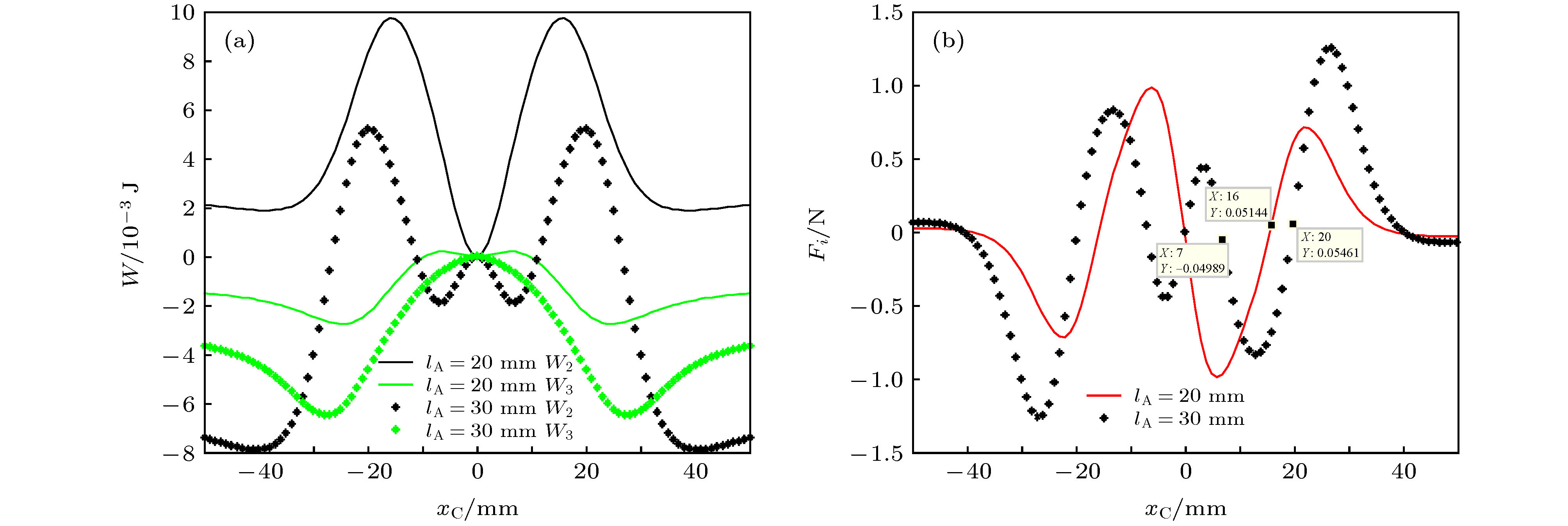图 14 (a) l_A = 20 mm和l_A = 30 mm时, W₂和W₃随x_C的变化关系;(b) l_A = 20 mm和l_A = 30 mm时, F_i随x_C的变化
Figure14. (a) The curves of W₂ and W₃ varying with x_C when l_A = 20 mm and l_A = 30 mm; (b) the curves of F_i varying with x_C when l_A = 20 mm and l_A = 30 mm.

从图13(b)和图14(a)可以看出, 系统势函数由三稳状态变为四稳状态, 主要是由于${W_2}$的形状的改变引起的, 而${W_2}$是由竖直方向的力${F_i}$决定的. 图14(b)中的红色实线和黑色星号点线分别是两尺寸矩形磁铁的${F_i}$随${x_{\rm{C}}}$的变化关系. 观察图14(b), 当${x_{\rm{C}}}$位于x轴正向(或负向)的0—15 mm之间时, l_A = 20 mm的矩形磁铁受到的作用力${F_i}$为负值(或正值), 这使得矩形磁铁始终被吸引向${x_{\rm{C}}} = 0$点移动, 从而使系统的${x_{\rm{C}}} = 0$点成为稳态点; 同理, 对于l_A = 30 mm的矩形磁铁, 由图14(b)的受力状态不难理解, 在0— ± 7 mm之间矩形磁铁在${x_{\rm{C}}} = 0$点始终受到排斥力而离开, 所以矩形磁铁不能稳定在${x_{\rm{C}}} = 0$点处. 但是当${x_{\rm{C}}}$在7—20 mm或$ - 20$—$ - 7$ mm之间时, l_A = 30 mm的矩形磁铁与环形磁铁间呈现出吸引状态, 所以悬臂梁在x_c = ± 7 mm附近会分别存在一个稳定点. 因此, 当l_A由20 mm变成30 mm时, 系统在${x_{\rm{C}}} = 0$处由一个势阱变成一个势垒, 并在x_c = ± 7 mm处多出两个势阱, 系统由三稳状态变为四稳状态.
由此可见, 在弹性恢复力一定时, 系统的稳态形式发生变化是两磁铁间竖直方向上的吸引力、排斥力区间发生变化所造成的.
2 -->

4.4.稳态点个数的验证

为验证上述势函数的分析, 分别从实验和动力学的角度考察系统的稳态特性. 选取表1参数对应的悬臂梁、环形磁铁和矩形磁铁, 构建双磁铁非线性悬臂梁结构, 如图15所示. 调节磁铁间距为d = 6 mm, 可以观察到系统的三稳特性, 这里只给出了3个稳态位置中的中稳态点和上稳态点, 根据对称性可知下稳态点.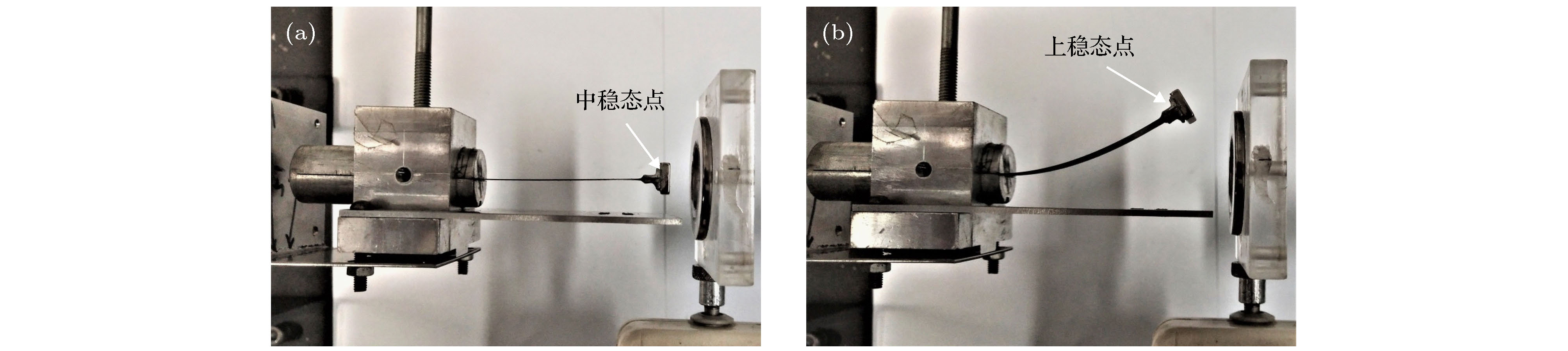
图 15 三稳结构　(a)中稳态点; (b)上稳态点
Figure15. The structure concluding three stable points: (a) The middle state point; (b) the upper stable point.

将图15中10 mm × 10 mm × 3 mm尺寸的矩形磁铁替换为30 mm × 30 mm × 3 mm尺寸的矩形磁铁, 其他参数不变, 可以观察到系统的四稳特性, 这里只显示悬臂梁上半部分的两个稳态位置: 上1稳态点和上2稳态点, 如图16所示. 根据对称性可知悬臂梁下半部分的两个稳态位置.
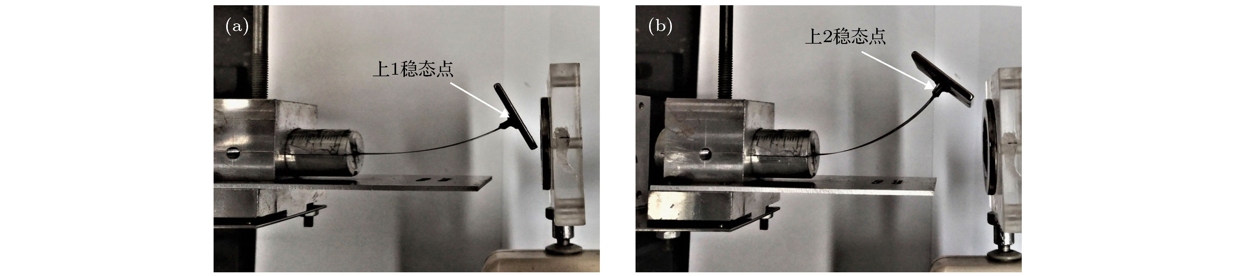图 16 四稳结构　(a)上1稳态点; (b)上2稳态点
Figure16. The structure concluding four stable points: (a) The upper stable point 1; (b) the upper state point 2.

与图13比较可知, 图15和图16的实验结果验证了势函数分析的有效性.
取(1)式中的P_A为0—120 Hz的宽带随机激励, 其强度Q由激励的方差表示. 根据表1参数以及(2)式—(8)式, 为较好地展现系统的响应特性, 取机械阻尼比${\xi _{\rm{r}}} = 0.0732$、激励强度Q = 0.06, 可计算得到磁铁间距d = 6 mm时系统的三稳振动响应的时域波形和相位图, 如图17所示.
图 17 三稳振动响应　(a)时域图; (b)相位图
Figure17. The vibration response of the tri-stable cantilever beam: (a) The time domain chart; (b) the phase chart.

将图17中的矩形磁铁尺寸替换为30 mm × 30 mm × 3 mm, 调整激励强度为Q = 0.45, 可以得到系统的四稳振动响应的时域波形和相位图, 如图18所示.
图 18 四稳振动响应　(a)时域图; (b)相位图
Figure18. The vibration response of the quad-stable cantilever beam: (a) The time domain chart; (b) the phase chart.

从图17和图18的结果可以看出, 动力学仿真得到的稳态点个数与势函数分析得到的稳态点个数相一致.

以永磁铁构成的常规非线性多稳态悬臂梁系统, 若要增加稳态数目, 通常需引入更多的磁铁, 易使系统结构变复杂和参数增多. 本文利用矩形磁铁和环形磁铁的作用, 提出了一种双磁铁实现多稳态的悬臂梁结构, 通过对该双磁铁悬臂梁结构的研究, 得到了以下主要结论.
1) 悬臂梁自由端的矩形磁铁与外部固定的环形磁铁同极相对所构成的双磁铁悬臂梁系统, 可通过改变磁铁尺寸或磁铁间距, 使系统具有单稳、双稳、三稳、四稳特征.
2) 对于一定尺寸的环形磁铁, 选取不同尺寸的矩形磁铁, 系统的势函数随磁铁间距的变化会出现不同稳态的转化方式. 当矩形磁铁尺寸取某一较小值时, 系统势函数会在三稳和单稳状态之间直接转化; 当增大矩形磁铁尺寸至某一值时, 系统势函数会出现三稳-双稳-单稳状态之间的转化现象; 当再增大矩形磁铁尺寸至更大值时, 系统势函数会出现四稳-双稳-单稳状态之间的转化现象.
3) 当环形磁铁的尺寸一定, 且选取一定的磁铁间距时, 矩形磁铁尺寸的变化, 还会引起系统势函数在单稳-三稳-四稳状态之间的转化.
4)系统势函数稳态数目发生转化的原因在于, 悬臂梁自由端运动时, 磁铁尺寸和间距的变化, 导致两磁铁间竖直方向上的吸引力、排斥力区间发生了变化.