Center for Soft Condensed Matter Physics and Interdisciplinary Research, School of Physical Science and Technology, Soochow University, Suzhou 215006, China
Abstract:In biological active systems there commonly exist active rod-like particles under elastic confinement. Here in this work, we study the collective behavior of self-propelled rods confined in an elastic semi-flexible ring. By changing the density of particles and noise level in the system, It is clearly shown that the system has an ordered absorbing phase-separated state of self-propelled rods and the transition to a disordered state as well. The radial polar order parameter and asphericity parameter are characterized to distinguish these states. The results show that the gas density near the central region of the elastic confinement has a saturated gas density that co-exists with the absorbed liquid crystal state at the elastic boundary. In the crossover region, the system suffers an abnormal fluctuation that drives the deformation of the elastic ring. The non-symmetric distribution of particles in the transition region contributes significantly to the collective translocation of the elastic ring. Keywords:active matter/ self-propelled rod/ absorption phase separation/ saturation density
2.模拟模型和方法模拟一个二维平面下的系统, 如图1(a)所示, 该系统由两部分组成: 其一是${N_{\rm{r}}}$个原长为${L_{\rm{r}}}$的自驱动杆状粒子; 另一部分是一条柔性环, 由${N_{\rm{l}}}$个原长为${L_{\rm{l}}}$的杆首尾链接而成, 柔性环将所有自驱动杆状粒子约束在其内部. 图 1 (a)系统组成的示意图, 颜色代表杆身的取向; (b)杆间碰撞受力示意图 Figure1. (a) The schematic diagram of this system, and the rods are colored according to their angle with respect to the radial direction; (b) the interaction between rods.
3.模拟结果和讨论封闭空间中的自驱动粒子倾向于在边界附近聚集[30-34]. 不同于球状粒子, 本文模型由杆状粒子组成. 由图2中的快照可以看出, 这样的自驱动杆在柔性环附近形成比较规则的极化液晶态排列. 由于杆粒子间向列型的相互作用, 整个柔性环内的自驱动杆状粒子基本是中心对称分布的, 此时用系统平均取向模的大小表示整体的极性程度, 柔性环内反向粒子的取向相互抵消, 系统的极性序接近于零. 但从快照上可以看出, 内部自驱动杆状粒子无序分布和有序聚集在环边界上是两种不同的分布, 而这两种分布的极性序都接近零无法很好地区分开. 图 2 三种典型分布的快照, 自驱动杆粒子数${N_{\rm{r}}}$均为1500, 噪声大小$\eta $分别为0.10, 0.20和0.50, 依次对应 (a)自驱吸附有序态、(b)过渡态和(c)无序态. 粒子颜色代表取向, 同图1 Figure2. The snapshots of three regions with fixed particle number ${N_{\rm{r}}} = 1500$ for different noise levels, and, respectively, with (a) $\eta = 0.10$, self-propelled particle absorbed ordered region, (b) $\eta = 0.20$ transient region, and (c) $\eta = 0.50$ disordered phase. The color represents the radial direction as Fig.1.
本文主要研究体系的密度和噪声对系统形态的影响. 系统改变自驱动杆的粒子数${N_{\rm{r}}}$和杆端的噪声强度$\eta $, 测量各参数空间点的径向极性序${S_{\rm{P}}}$的值, 可以得到如图3(a)所示的相图. 明显地, 根据极性序${S_{\rm{P}}}$值的大小, 相图中从最左边极性序${S_{\rm{P}}}$接近1的有序相区域, 逐渐过渡到右侧极性序${S_{\rm{P}}}$接近0的无序区. 有序区主要集中在粒子数${N_{\rm{r}}}$较大, 噪声强度$\eta $较低的区域, 对应的快照如图2(a)所示. 大部分的自驱动杆状粒子都指向环外方向, 集中排列在柔性环上, 且可以构成完整的层状分布. 同时剩余的粒子在中心区域形成角度和位置都比较均匀地分布. 无序区域则主要分布在粒子数${N_{\rm{r}}}$较小或噪声强度$\eta $较大的区域, 如图2(c)所示, 其内部自驱动粒子的取向是无序的, 均匀分布在环内. 过渡区间主要分布在这两相之间的区域, 如图2(b)所示, 外层的自驱动杆无法形成完整的层状稳定排布, 而分别集中成反向的两个集团或异向的多个集团. 外侧的柔性环也因此有明显的变形, 中心区域同样存在一定密度的比较均匀的无序气态分布. 图 3 改变噪声强度$\eta $和弹性环中自驱动杆粒子数${N_{\rm{r}}}$得到的相图 (a)比较径向极性序参${S_{\rm{p}}}$大小得到的热力图; (b)比较非球度$\varDelta $大小得到的热力图, 其中转变区域具有极大值 Figure3. Phase diagrams for self-propelled rods in elastic-ring with varying the noise strength $\eta $ and the number of self-propelled rods ${N_{\rm{r}}}$, and the order parameter corresponding to (a) the radial polarity ${S_{\rm{P}}}$ and (b) the asphericity $\varDelta $. We have maximal asphericity $\varDelta $ in the transition region.
约化密度差P的值越大说明系统内外两侧粒子分布的密度差异越大, P值越接近0则对应系统内部的粒子分布越均匀. 通过计算系统的约化密度差可以得到如图4(a)所示的热度图, 低噪声有序区域明显对应的区域约化密度差P值较高, 高低密度两相分离明显. 高噪声无序相区域的P值很低, 接近均匀分布. 这与图2快照中的粒子分布是一致的. 可以看到约化密度差P与极性序${S_{\rm{P}}}$有类似的分布, 随着噪声强度$\eta $的减弱, 系统从无序相进入有序相的过程中, 柔性环附近内部粒子的堆积程度也相应增强. 极性序${S_{\rm{P}}}$主要由环附近堆积的粒子贡献, 而自驱动粒子在环边界的堆积程度由约化密度差P刻画, 所以极性序${S_{\rm{P}}}$的大小一定程度上与约化密度差P正相关. 图 4 (a)改变噪声强度$\eta $和自驱动杆粒子数${N_{\rm{r}}}$, 比较约化密度差P得到的热力图; (b)不同噪声强度$\eta $下, 弹性环中心附近粒子数密度随自驱动杆粒子数${N_{\rm{r}}}$的变化趋势 Figure4. (a) Phase diagram of the reduced density difference P for self-propelled rods with varying the noise strength $\eta $ and the number of self-propelled rods ${N_{\rm{r}}}$; (b) density of central particles, ${\psi _{{\rm{in}}}}$, versus the particle number ${N_{\rm{r}}}$ for different noise strength $\eta $.


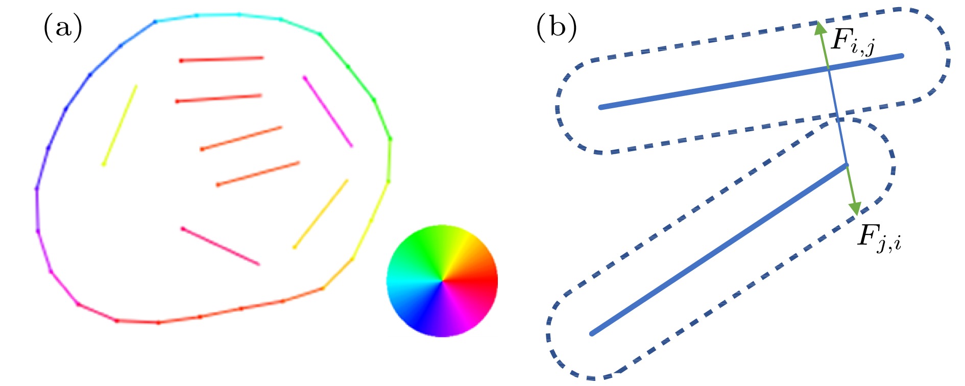 图 1 (a)系统组成的示意图, 颜色代表杆身的取向; (b)杆间碰撞受力示意图


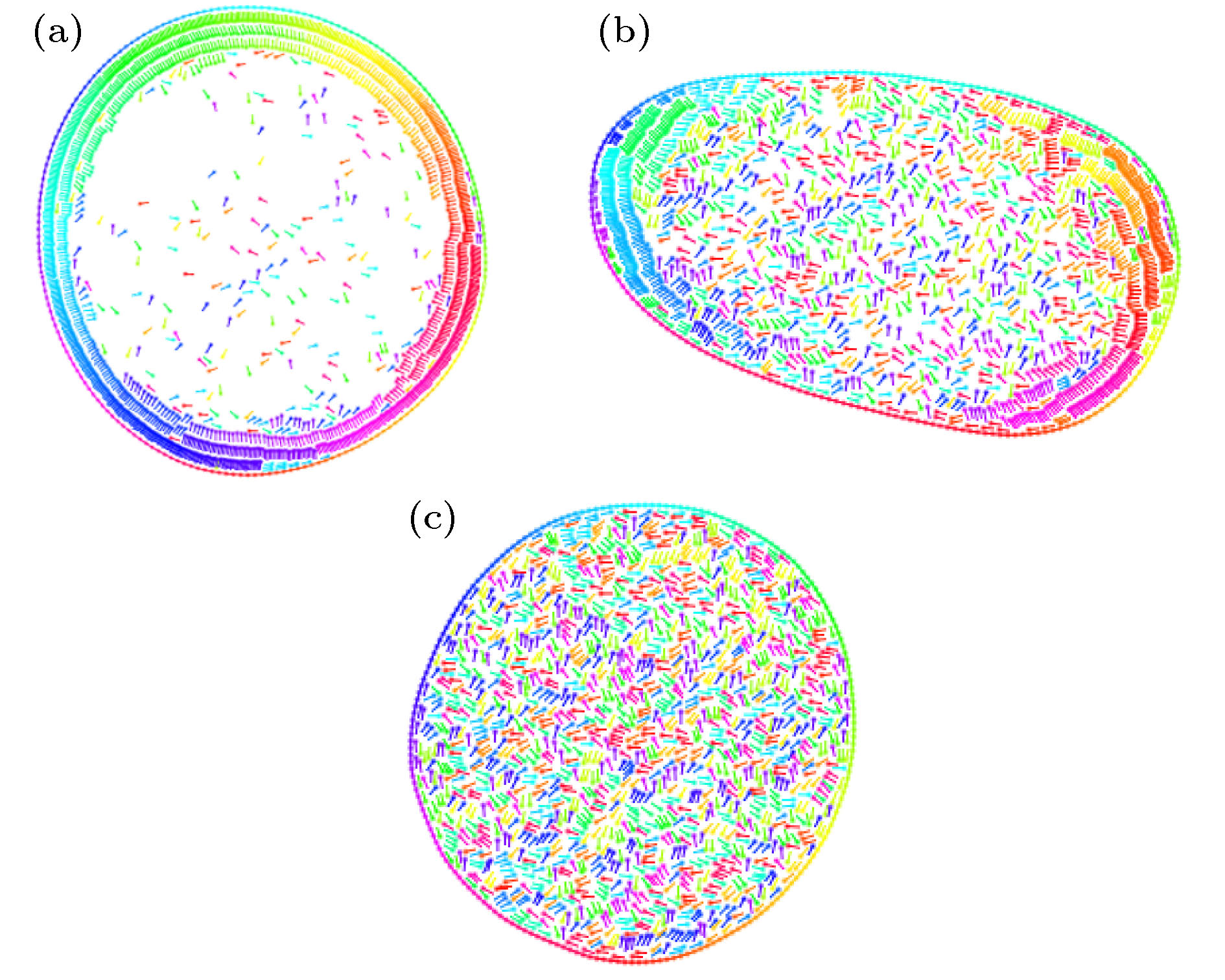 图 2 三种典型分布的快照, 自驱动杆粒子数


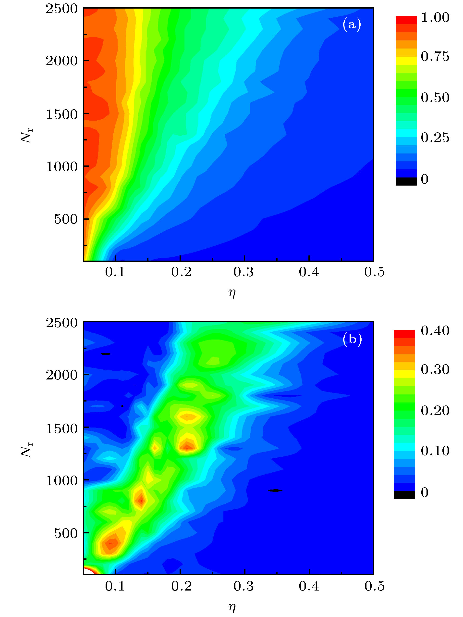 图 3 改变噪声强度


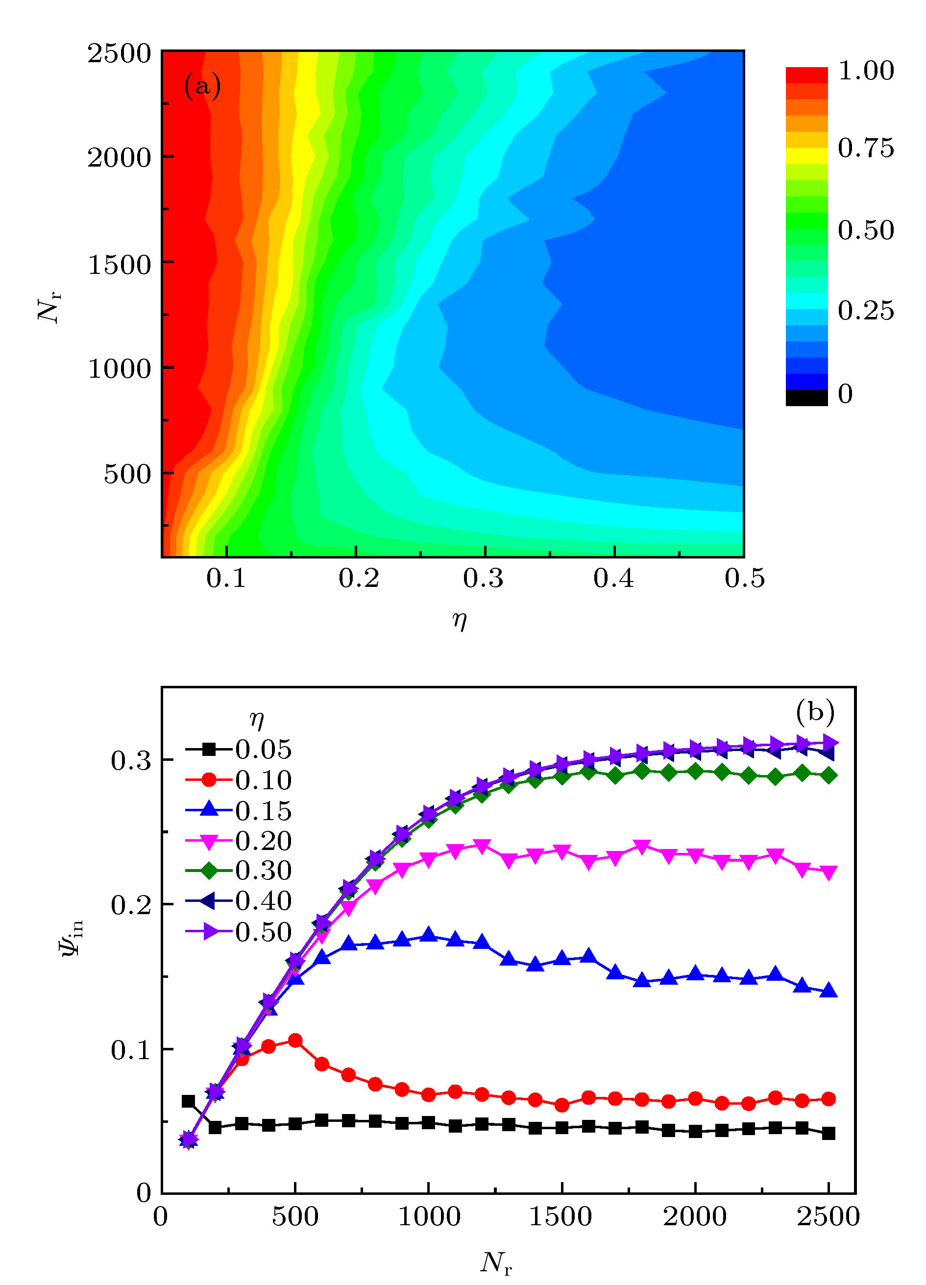 图 4 (a)改变噪声强度


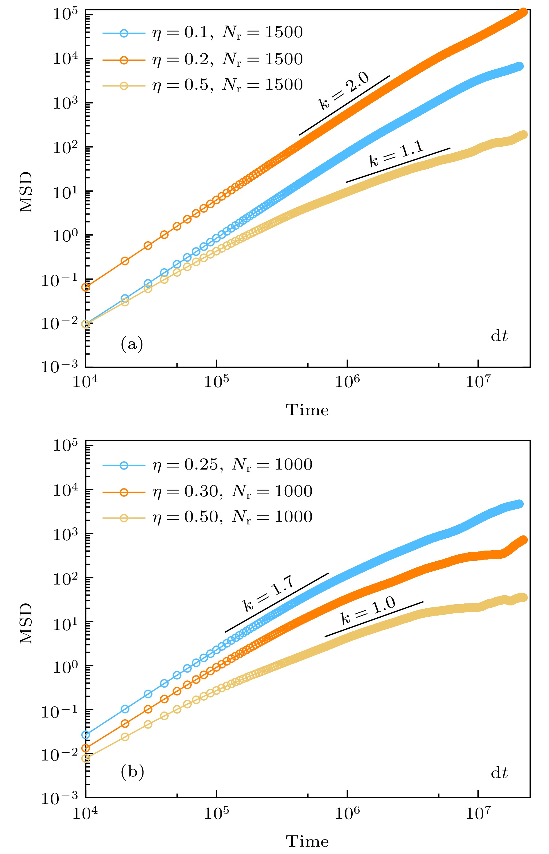 图 5 弹性环及杆状粒子质心均方位移随时间的变化 (a)粒子数


