Abstract:At present, numerical methods applied to the coupling analysis of transmission lines on the lossy dielectric layer excited by ambient wave are still rare in the literature. As a temptation to fill this gap, a novel time domain hybrid method is proposed, in which the modified transmission line (TL) equations, finite-difference time-domain (FDTD) method, and some interpolation schemes are organically combined together. It can overcome the difficulty in building the coupling model of ambient wave to transmission lines on the lossy dielectric layer greatly. In this method, the modified transmission line (TL) equations suitable for the coupling analysis of multi-conductor transmission lines (MTLs) on the lossy dielectric layer are derived from the traditional TL equations firstly. Compared with the traditional TL equations, the electromagnetic fields in the lossy dielectric layer are introduced into the equivalent distribution sources of modified TL equations. Generally, the precision of TL equations is dependent on the accuracy of equivalent distribution sources, which are obtained from the incident electric fields parallel and perpendicular to the MTLs. Therefore, the FDTD method is utilized to model the structure of lossy dielectric layer to calculate the electromagnetic field distribution surrounding the MTLs and in the dielectric layer. Since the heights and distances of MTLs can be arbitrary values, the electric fields parallel and perpendicular to the MTLs cannot be obtained from the electric fields on the edges of FDTD grids directly, which should be computed via some interpolation schemes. Then the modified TL equations are established, which should be solved by the central difference scheme of FDTD method to obtain the voltages and currents on the MTLs and terminal loads. The significant feature of this proposed method is that it can realize the synchronous calculations of electromagnetic field radiation and transient responses on the MTLs. Finally, numerical simulations of single and multiconductor transmission lines on the lossy dielectric layer excited by ambient wave at different incident angles are employed to exhibit the accuracy and efficiency of the proposed method by comparing with the simulation software CST. Because the structures of MTLs do not need to be meshed, the proposed method outperforms the simulation software CST in both memory usage and computation time. Keywords:transmission lines on the lossy dielectric layer/ modified transmission line equations/ interpolation schemes/ finite-difference time-domain method
$\frac{{\rm{d}}}{{{\rm{d}}y}}V\left( y \right) + LI\left( y \right) = - \frac{{\rm{d}}}{{{\rm{d}}y}}{E_{\rm{T}}}\left( y \right) + {E_{\rm{L}}}\left( y \right),$
其中,
${E_{\rm{T}}}\left( y \right) = \int_{\rm{0}}^{d + h} {E_z^{{\rm{inc}}}\left( y \right){\rm{d}}z},$
对(9)式右边的两项应用高斯定律可得${\rm{j}}\omega \displaystyle\mathop{{\int\!\!\!\!\!\int}\mkern-21mu \bigcirc}\nolimits_S {\varepsilon {{{E}}^{{\rm{inc}}}} \cdot {\rm{d}}{{S}}} = {\rm{0}}$和${\rm{j}}\omega \displaystyle\mathop{{\int\!\!\!\!\!\int}\mkern-21 mu \bigcirc}\nolimits_S {\varepsilon {{{E}}^{{\rm{sca}}}} \cdot {\rm{d}}{{S}}} = {\rm{j}}\omega q\left( y \right)$, 其中$q\left( y \right)$为传输线沿线的电荷密度. 电荷密度$q\left( y \right)$与散射电压${V^{{\rm{sca}}}}\left( y \right)$和传输线单位长度电容C之间满足关系: $q\left( y \right) = C{V^{{\rm{sca}}}}\left( y \right)$. 而散射电压可由总电压和入射电场表示为
${V^{{\rm{sca}}}}\left( y \right) = V\left( y \right) - {V^{{\rm{inc}}}}\left( y \right) = V\left( y \right) + \int_0^{d + h} {E_z^{{\rm{inc}}}\left( y \right)} {\rm{d}}z.$
3.数值仿真与分析采用时域混合算法对有耗介质层上单导体传输线和多导体传输线的电磁耦合进行数值模拟, 并与商业电磁仿真软件CST的计算结果进行对比, 来验证算法的正确性和高效性. 算例1 有耗介质层上单导线的电磁耦合模型如图5所示, 有耗介质层大小为0.2 m × 0.4 m, 厚度为0.01 m, 相对介电常数为10, 电导率为20 S/m. 单导线长度为20 cm, 高度为1.9 cm, 端接负载分别为50和100 Ω. 入射波为高斯脉冲垂直照射单导线, 幅度为1000 V/m, 脉宽为2 ns. 为了保证计算精度, 时域混合算法选用的网格大小为5 mm. 在计算空间电磁场分布时, 选用各向异性介质完全匹配层(UPML)截断边界, 入射波距离多导线的高度为4个空间网格大小. 图6给出了时域混合算法与CST微波工作室计算得到的负载R2上的电压响应对比曲线. 可以看出, 两种方法的计算结果振荡周期保持一致, 且幅值吻合度非常高. 表1列出了两种算法计算所需内存和时间的对比, 可以看出, 时域混合算法相较于CST, 节省了47%左右的计算时间, 是因为时域混合算法无需对单导线直接建模. 这里需要说明的是, CST软件虽然提供线缆工作室模拟传输线的电磁耦合, 但是只适用于接地面为金属体的情况. 图 5 有耗介质层上单导线的电磁耦合模型 Figure5. Coupling model of single transmission line on the lossy dielectric layer.
图 6 负载R2上的电压响应 Figure6. Voltages on the load R2 computed by the two methods
方法
内存/MB
计算时间/min
CST
63
19
时域混合算法
34
10
表1两种方法计算算例1时所需内存和时间对比 Table1.Memories and computation time needed by the two methods for the first example.
算例2 有耗介质层上多导体传输线的电磁耦合模型见图7, 有耗介质层的大小为0.4 m × 0.7 m, 厚度为0.01 m, 相对介电常数为10, 电导率为50 S/m. 5根导线平行放置在有耗介质层上, 长度为0.5 m, 高度为1.1 cm, 间距为4 mm, 半径为1 mm. 始端负载R1—R5均为50 Ω, 终端负载R6—R10均为100 Ω. 入射波类型和算法选用的网格大小与算例1的相同. 图 7 有耗介质层上多导体传输线的电磁耦合模型 Figure7. Coupling model of multi-conductor transmission lines on the lossy dielectric layer.
首先, 入射波角度设置为θ = 180°, ? = 90°和α = 180°, 即垂直照射多导线. 采用时域混合算法与电磁仿真软件CST计算得到负载R1和R7上的电压响应对比曲线, 如图8所示. 可以看出, 两种算法的计算结果基本保持一致. 图 8 入射波垂直照射下的多导线端接负载的电压响应 (a)负载R1上的电压; (b)负载R7上的电压 Figure8. Voltages on the terminal loads of multi-conductor transmission lines under the condition of ambient wave perpendicular to the multi-conductor transmission lines: (a) Voltages on R1; (b) voltages on R7.
表2两种方法计算算例2时所需内存和时间对比 Table2.Memories and computation time needed by the two methods for the second example.
图 9 入射波斜照射下的多导线端接负载的电压响应 (a)负载R1上的电压; (b)负载R7上的电压 Figure9. Voltages on the terminal loads of multi-conductor transmission lines under the condition of ambient wave oblique to the multi-conductor transmission lines: (a) Voltages on R1; (b) voltages on R7.

 图 1 闭合回路和闭合曲面的选取


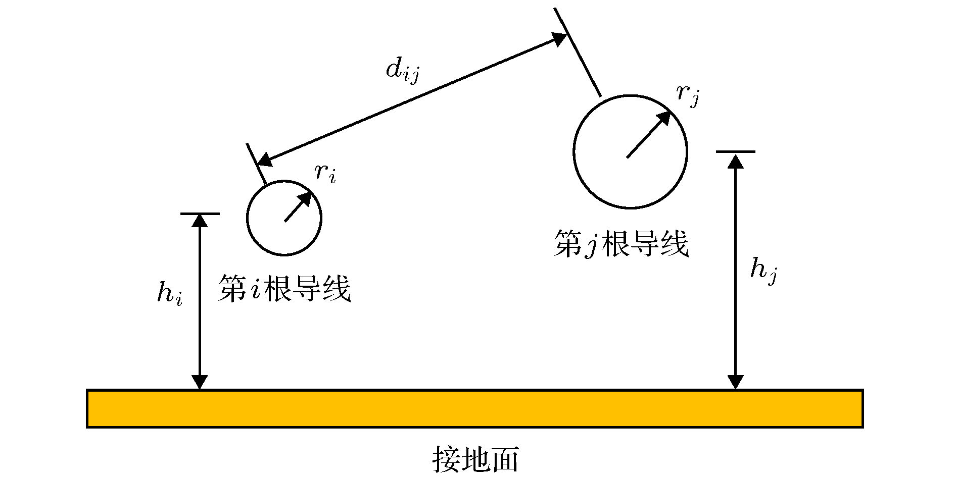 图 2 多导体传输线的横截面几何结构
 图 3 多导线沿线和垂直电场分量的插值示意图


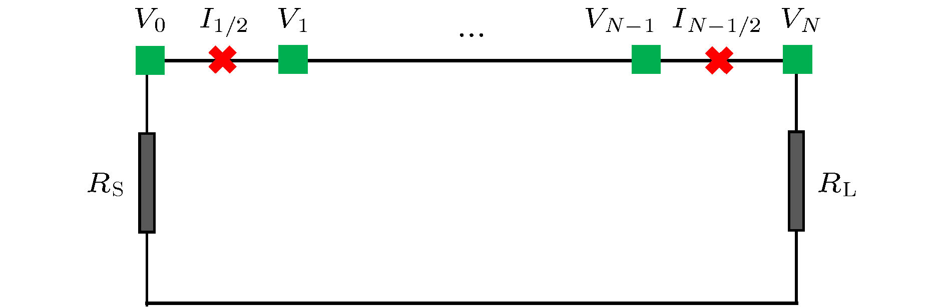 图 4 传输线的FDTD网格划分
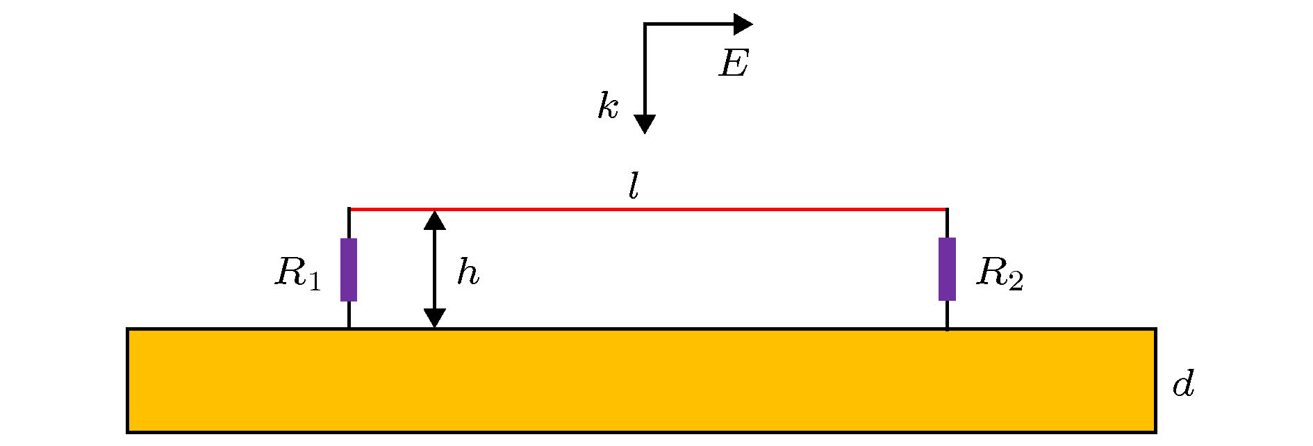 图 5 有耗介质层上单导线的电磁耦合模型
 图 6 负载R2上的电压响应
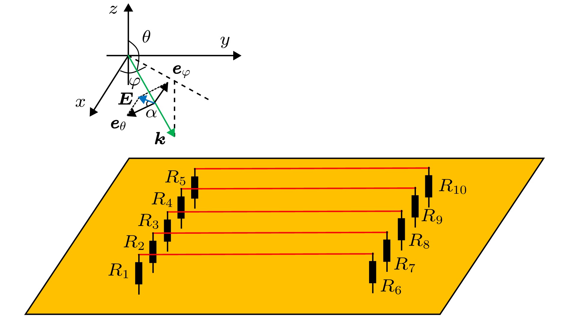 图 7 有耗介质层上多导体传输线的电磁耦合模型
 图 8 入射波垂直照射下的多导线端接负载的电压响应 (a)负载R1上的电压; (b)负载R7上的电压
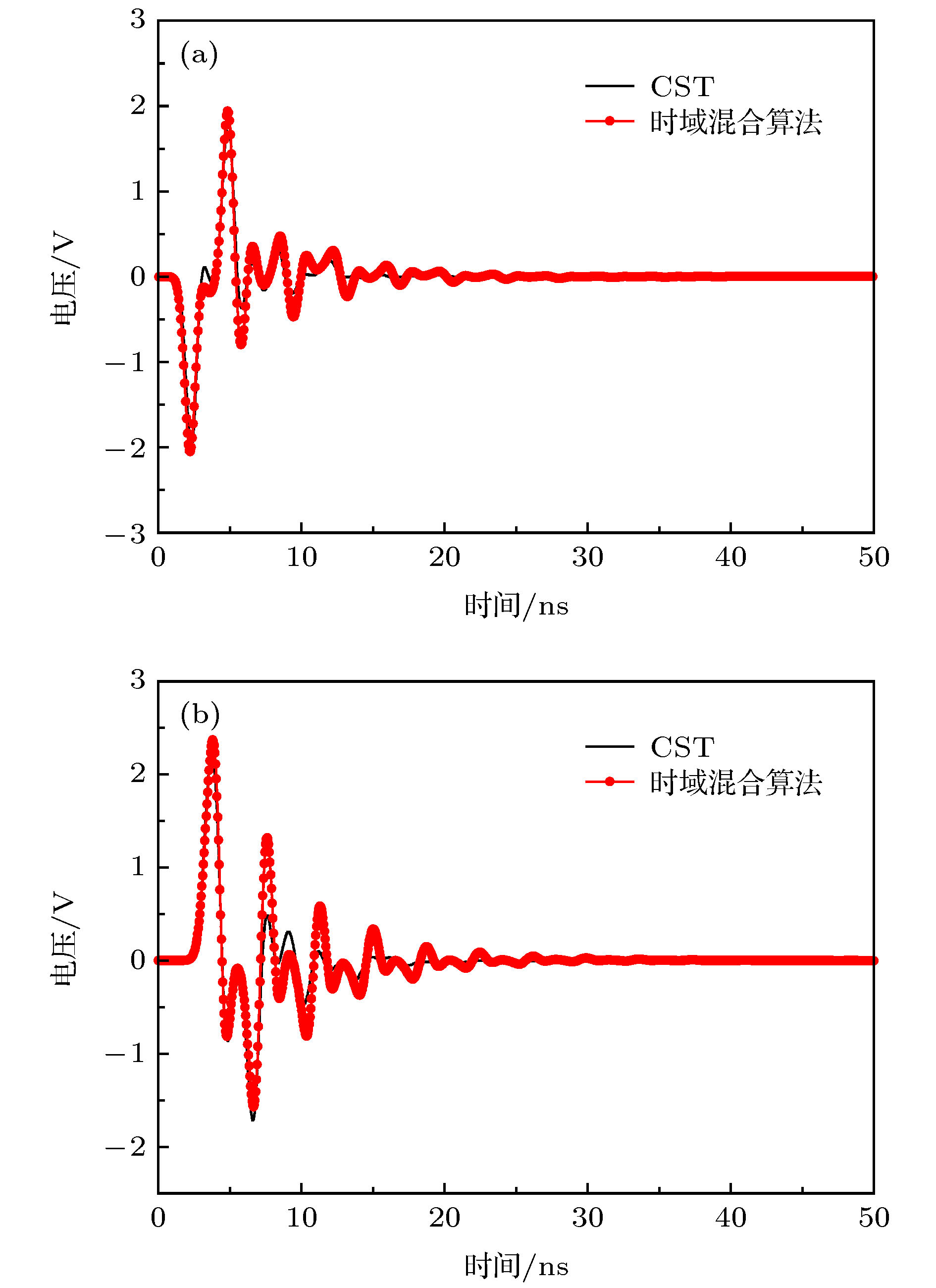 图 9 入射波斜照射下的多导线端接负载的电压响应 (a)负载R1上的电压; (b)负载R7上的电压