HTML
--> --> -->The BLH is difficult to be directly measured. However, at a well-mixed layer top, there are usually significant increases in potential temperature, depolarization ratio, and horizontal wind speed or decreases in relative humidity, aerosol concentration, and turbulence intensity (Li et al., 2017). Based on these characteristics, various BLH definitions and retrieval methods have been developed, such as ideal profile fitting (Steyn et al., 1999), maximum variance (Hooper and Eloranta, 1986), first gradient (Flamant et al., 1997), threshold (Melfi et al., 1985), wavelet transform (Cohn and Angevine, 2000), and the combination method of wavelet transform and image processing (Lewis et al., 2013).
Numerous instruments have been applied in detecting the BLH, including in situ instruments such as radiosondes mounted on masts or balloons (Guo et al., 2016) and remote sensing instruments such as microwave radiometers (Coen et al., 2014), wind profilers (Cohn and Angevine, 2000), sodars (Emeis et al., 2007), lidars (Yang et al., 2020), and satellites (Luo et al., 2016). The advantages and shortcomings of these instruments are summarized by Seibert et al. (2000). Among these, coherent Doppler wind lidar (CDWL) is widely applied in detecting wind and rain (Wei et al., 2019), turbulence (O’Connor et al., 2010; Banakh et al., 2017; Leung et al., 2018), and ABL classification (Manninen et al., 2018; Yuan et al., 2020). Its high spatial and temporal resolutions make the CDWL one of the most promising instruments in detecting BLH (Wang et al., 2018).
BLH can be detected by using one of the CDWL measurements as a tracer: for example, horizontal wind speed (Emeis et al., 2008), the aerosol-related parameter such as aerosol backscatter coefficient or carrier-to-noise ratio (CNR) (Pe?a et al., 2013), or the turbulence-related parameter such as vertical wind speed variance or turbulent kinetic energy dissipation rate (TKEDR) (Vakkari et al., 2015; Huang et al., 2017; Banakh et al., 2020). The aerosol-based BLH is found to be higher than the turbulence-based BLH with an overestimation of several hundred meters both in the morning and the late afternoon due to different BLH definitions (Schween et al., 2014). Besides, differences of up to one kilometer between the two kinds of BLHs are observed, which raises great concern. A reasonable assumption is that the CNR is distorted, leading to an incorrect BLH value. In theory, CNR is an indicator of aerosol concentration and thus can be used to retrieve BLH. In practice, CNR could be distorted by instrument instability. For a single CDWL, it is hard to prove whether the CNR change is a natural variation introduced by aerosol concentration variation or an abnormal deviation caused by instrument instability. Thus, an intercomparison experiment is designed with two identical CDWLs, where only one lidar is equipped with a stability control subsystem. The lidar with stability control can be used as a reference. Note that the instrument stability is difficult to be controlled in a harsh environment or for long-term observations. Even minor instrument instability will result in a BLH bias. Thus, a robust solution is expected to be found.
In this work, an intercomparison experiment is carried out to analyze the effect of instrument instability on BLH bias. A robust solution for detecting BLH with CDWL is provided. The experimental site, instruments, and data are introduced in section 2. Section 3 describes the BLH retrieval methods. Section 4 presents the lidar observation results and BLH retrieval results. A statistical comparison of the BLHs derived from the two lidars is also performed. Finally, a conclusion is given in section 5. If not specified, LST (Local Standard Time, LST = UTC + 8) is used.
Two all-fiber micro-pulse CDWLs are located as shown in Fig. 1. The lidars have full hemispheric scanning capability with a rotatable platform. As two D-shaped aspheric lenses are glued together with aligned optical axes, the overlap distance and the blind zone are 1 km and 30 m, respectively. Below 2.2 km, the vertical resolution is set to 26 m for studying the fine structure. Above 2.2 km, the aerosol concentration is usually low, and the vertical resolution is set to 52 m for improving the detection probability. The key parameters are listed in Table 1. The detailed specifications and the error analysis of radial velocity have been described by Wang et al. (2017). Only CDWL1 is equipped with a temperature stabilizing module. It is composed of two thermoelectric coolers (TEC) and a bottle of cryogen which is connected with the heat-conducting pipes wrapping around the telescope. A proportional-integral-differential algorithm is developed to control the TEC and the valve of the cryogen. A package made of a heat-insulating material is used to guarantee the temperature of telescope. The telescope temperature is controlled at 25°C with a fluctuation of 0.5°C.
 Figure1. The two CDWLs used in the experiment.
| Parameter | Value | |
| Laser | Wavelength (nm) | 1548 |
| Pulse energy (μJ) | 100 | |
| Repetition frequency (kHz) | 10 | |
| Telescope | Diameter (mm) | 80 |
| Scanner | Zenith scanning range (°) | 0?90 |
| Azimuth scanning range (°) | 0?360 | |
| Radial temporal resolution (s) | 2 |
Table1. Key parameters of the CDWLs.
The two lidars operate simultaneously for 12 days and separately for the remaining days of the observation period. During the experiment, CNR, wind vector, and TKEDR are simultaneously measured with a velocity azimuth display scanning mode, which is defined as conical scanning by a laser beam around the vertical axis with a fixed zenith angle of 30° (Sathe and Mann, 2013). The azimuth angle resolution is 5° and the period of one scan is about 144 s. For every radial measurement during one scan, the atmospheric backscatter signal received by the telescope is mixed with a local oscillator, resulting in a radio frequency beating signal. After Fourier transformation, the Doppler shift caused by the radial velocity can be retrieved. The ratio of the beating signal power to noise power over the entire spectral bandwidth is the radial CNR (Wang et al., 2017). The CNR is an average of radial CNRs over one scan. Then, the wind vector is determined from the sine dependence of radial velocity versus azimuth angle. After filtering out the invalid radial velocities, the vector is obtained by achieving the maximum of the filtered sine wave fitting function (Banakh et al., 2010). Finally, TKEDR can be estimated by fitting the azimuth structure function of radial velocity to a model prediction. The algorithm, including error analysis, is demonstrated by Smalikho and Banakh (2017). Note that the accuracy of wind and TKEDR mainly depends on CNR.
3.1. Retrieval of BLH from CNR
The aerosol concentration in the ABL is much higher than that in the free atmosphere, resulting in a decrease in aerosol backscatter signal at the boundary layer top. CNR can be used as a measure of aerosol backscatter. One method for retrieving the BLH from CNR is the Haar wavelet covariance transform (HWCT) method. The Haar function is defined as (Brooks, 2003):where


where


Firstly, the CNR profile is range-corrected via multiplying by the square of distance. Secondly, a 7-min block average and a 250-m spatial smoothing are applied to mitigate the interferences from noise and small-scale events, respectively. Figure 2a shows a nighttime range-corrected CNR profile, which is normalized in the range of 0 to 4 km. Figure 2b shows the profile’s HWCT result, in which two local maximum positions (LMP) are found. Multiple LMPs demonstrate the complex aerosol structure, consisting of a lower SBL formed by radiative cooling from the ground and a higher RL containing former mixed layer air. There are usually decreases in aerosol backscatter at the tops of these layers. Based on the positions of the two LMPs, the SBL height (SBLH) of 1.82 km and the RL height (RLH) of 2.86 km are obtained. In the daytime, as shown in Fig. 2f, there is usually a single LMP, by which the ML height (MLH) of 2.81 km is obtained. Thirdly, a Different Thermo-Dynamic Stabilities algorithm is applied to make the BLH results more uniform under the full range of atmospheric stability conditions, especially under SBL (RL) conditions. The physical basis of this algorithm is to check the temporal continuity and vertical coherence of the BLH (Su et al., 2020).
 Figure2. The 7-min average profiles centered at 0853 LST 27 September 2019 of CDWL1: (a) Range-corrected CNR after normalization and its (b) HWCT result, (c) original CNR, (d) lg(TKEDR). Centered at 1311 LST 27 September: (e)–(h). The black dots denote the BLHs retrieved by the HWCT method. The blue dots are the BLHs retrieved by the CNR threshold method. The red squares are the BLHs retrieved by the TKEDR threshold method.
The performance of the HWCT method could be affected by a poorly defined boundary layer top or multiple aerosol layers. For example, RLH could be misclassified as SBLH. Thus, the other CNR threshold method, which is fast and has low uncertainty, is adopted in this study. This method is applied to the original CNR. The values of the thresholds are determined by using the retrieval results of the HWCT method as references. It can be seen from Fig. 3 that the optimal thresholds for SBLH/MLH and RLH are –25 dB and –32 dB, respectively. By testing, the values are also found to be suitable for the other days during this observation period. If not specified, the CNR method discussed in the following sections denotes the CNR threshold method.
 Figure3. The linear regression of the BLH retrieved by using different CNR thresholds as a function of that by the HWCT method: (a) Determination coefficient (R2) (black dashed line) and root-mean-square error (RMSE) (red line) for SBLHCNR/MLHCNR. (b) Similar to (a) but for RLHCNR.
2
3.2. Retrieval of BLH from TKEDR
At a well-mixed layer top, there is an entrainment zone between the ML and the free atmosphere. In this zone, materials are not fully mixed, resulting from a decrease in turbulence intensity, which can be characterized by TKEDR. Thus, for a given averaging time and an appropriate threshold, the TKEDR above the ML top is less than the threshold and vice versa. A threshold of 10?4 m2 s?3 is applied here (Banakh et al., 2020). For example, Fig. 2d gives a TKEDR profile after a 7-min block average, and the MLH result is 0.31 km.As shown in Fig. 2h, the profile fluctuation from unexpected noise causes an outlier point, indicating that the retrieval suffers from occasional interference. To exclude the outlier point, a median algorithm is adopted. First, the median


4.1. Lidar observation results
The continuous observation results during 27–28 September are shown in Fig. 4, including CNR, horizontal wind speed and direction, vertical wind speed, and TKEDR. The left and right columns are the results of CDWL1 and CDWL2, respectively. The CNRs of the two lidars are quite different. To show the details, the radial profiles are plotted in Figs. 5a–j. The radial CNR of CDWL2 is much weaker than that of CDWL1 in the afternoon, and the worst case is found in Fig. 5e at 1400 LST. This phenomenon repeats each day, indicating association with diurnal atmospheric temperature variations. One reasonable explanation is that the optics of the telescope suffer aberrations due to the ambient temperature change, resulting in a loss in heterodyne efficiency (Chambers, 1997). In the CDWL, the atmospheric backscatter signal is coupled from free space into a polarization-maintaining fiber with a core diameter of 9 micrometers. The temperature variation may also change the focusing point due to the thermal expansion of the mechanical structures in the telescope.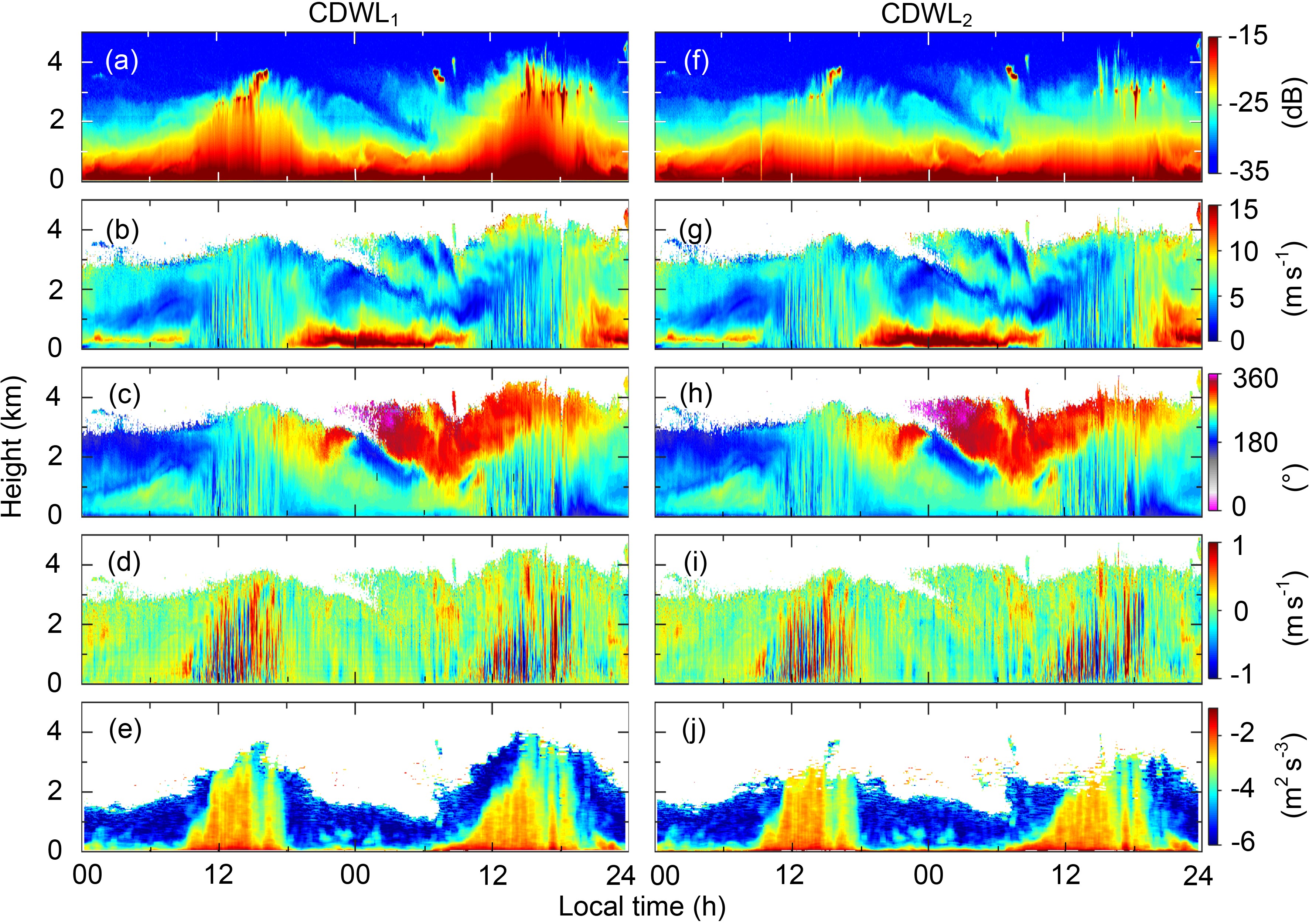 Figure4. Lidar observation results during 27–28 September 2019: (a) CNR, (b) horizontal wind speed, (c) horizontal wind direction, (d) vertical wind speed, (e) lg(TKEDR) of CDWL1. (f)–(j) Results of CDWL2. The horizontal wind direction is defined as 0° for northerly wind, rotating clockwise. Negative vertical wind speed denotes rising motion.
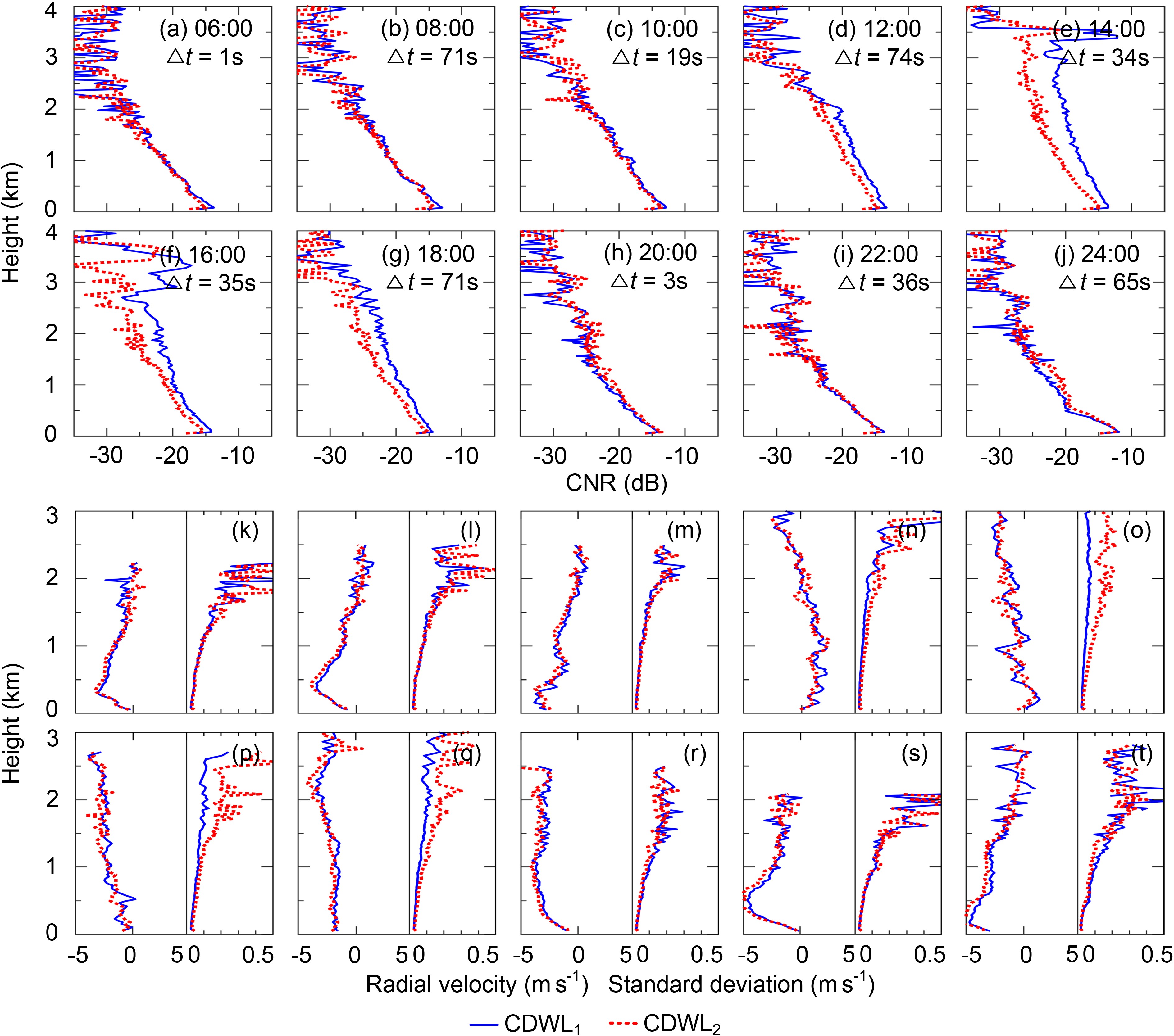 Figure5. (a)–(j) Radial CNR profiles at different measurement moments on 27 September. (k)–(t) The corresponding radial velocities and their standard deviation profiles. The △t values denote the moment difference between CDWL1 (blue line) and CDWL2 (red dashed line).
The corresponding radial velocities and their standard deviation profiles are plotted in Figs. 5k–t. Since the measurement moments of the two lidars are not the same (see Figs. 5a–j), small radial velocity differences are observed. As the standard deviation mainly depends on the radial CNR, to guarantee the accuracy of wind, the radial velocities with radial CNRs below –35 dB are abandoned (Wang et al., 2017). The accuracy of the wind measurements of CDWL1 has been validated by comparison with a radiosonde, and the mean differences in horizontal wind speed and direction are 0.3 m s?1 and 1.1°, respectively (Wei et al., 2019). Although the radial CNR of CDWL2 is weaker in the afternoon, most values are still valid for measuring the wind within the ABL. As shown in Fig. 6, the mean differences between the two lidars in horizontal wind speed, horizontal wind direction, and vertical wind speed are 0.08 m s?1, –0.16°, and –0.02 m s?1, respectively, indicating the accuracy of the wind measured by CDWL2.
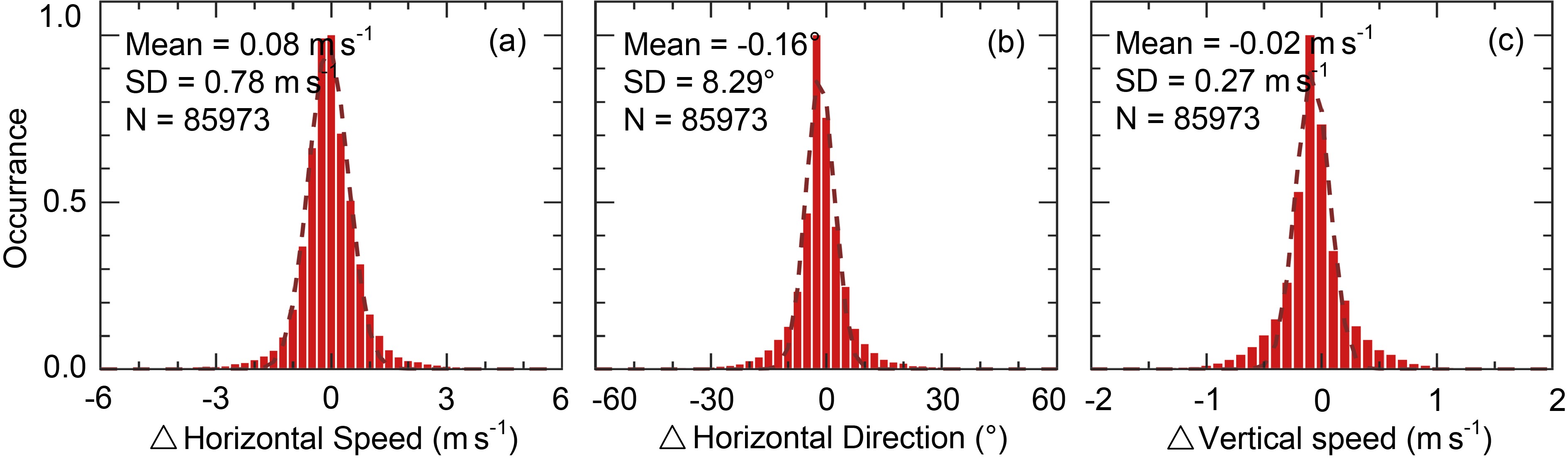 Figure6. Statistical analysis of the wind differences between the two lidars on 27 September: Histogram distributions of (a) horizontal wind speed difference, (b) horizontal wind direction difference, and (c) vertical wind speed difference. The dashed lines denote Gaussian fits.
2
4.2. BLH retrieval results
The BLH retrieval results during 27–28 September are shown in Fig. 7. The results are smoothed by finding the median with a 21-min window. The ABL can be classified by the gap between the SBLH from CNR and the MLH from TKEDR. In the morning, the ABL changes from the SBL (RL) into the ML when the gap is less than a specified value. In the late afternoon, the MLH departs from the SBLH, and the ML turns into the SBL (RL) again when the gap is larger than the value (Wang et al., 2019). For example, a specified value of 500 m is used on 27 September as the ML top is about 3 km. Figure7. BLH retrieval results during 27–28 September: (a) Results of CDWL1. (b) Results of CDWL2. SBLH/MLHCNR (blue dots) and RLHCNR (black open circles) are retrieved by the CNR method. MLHTKEDR (red squares) are retrieved by the TKEDR method.
The results of CDWL1 are plotted in Fig. 7a. The ABL experiences two obvious diurnal cycles, which evolve as illustrated in Coen et al. (2014). The sunrise and sunset times are marked by upward and downward arrows, respectively. Before sunrise on 27 September, the SBL is found to be capped by the RL. The SBLH and the RLH retrieved from CNR are around 1.5 km and 2.5 km, respectively. After sunrise, the ML develops gradually due to solar radiation and is well-mixed by turbulence. The SBL (RL) is finally merged into the developing ML at about 1200 LST. The MLH can be retrieved from both CNR and TKEDR. In principle, the MLH will keep steady if the temporal gradient of surface temperature is around zero in the afternoon. The fluctuation of the MLH from TKEDR is a result of the turbulence intensity variation related to the cloud-top radiative cooling. The ML departs from the SBL (RL) rapidly before sunset. After sunset, the SBL (RL) develops again. On 28 September, the BLH evolves as it did on 27 September, but the ML top is a little higher than on 27 September. This sequence of BLH evolution is typical for land surfaces in the midlatitudes (Kaimal and Finnigan, 1994). Note that at about 0200 LST 28 September, the sudden rise of the RLH from CNR is caused by an injection of aerosols, and a coinciding wind direction shear from the south to the northwest is observed (see Fig. 4c). This indicates that the retrieval of the BLH based on the vertical distribution of aerosols could be affected by multiple aerosol layers.
The accuracy of BLH detections of CDWL1 has been validated by comparison with a direct detection lidar (Wang et al., 2019). Thus, the results of CDWL1 are used as references in this study. Figure 7b plots the results of CDWL2. In the daytime on 27–28 September, the MLH from CNR of CDWL2 is much lower than that of CDWL1. This suggests that the performance of the CNR method is affected by the CNR deviation of CDWL2, resulting in the MLH bias. In contrast, since the wind measured by CDWL2 is accurate, as discussed in section 4.1, the accuracy of TKEDR estimated from wind is guaranteed. As a result, robust MLH from TKEDR of CDWL2 is observed.
2
4.3. Comparison of the BLHs derived from the two lidars
For quantitative analysis, a 12-day statistical comparison of the BLHs derived from the two lidars is performed.The scatter diagrams of the MLHs retrieved from CNR and TKEDR are shown in Figs. 8a–b. The results of CDWL2 are plotted versus those of CDWL1. The histogram distributions of the MLH bias are inserted in the bottom right corner of each panel. The negative bias means that the result of CDWL2 is lower than that of CDWL1. For the MLH from CNR, there are two gathering regions where normalized densities are larger than 0.5. The low gathering region that lies on the 1:1 line is a result of the calm days during this observation period, because weak convection leads to low ML tops; the high gathering region that deviates from the line results from the turbulent days. Table 2 presents the linear regression. The fit of these points to the 1:1 line shows the worst performance with the smallest determination coefficient (R2) of –2.50 and the largest root-mean-square error (RMSE) of 1.08 km. For the MLH from TKEDR, most points lie on the 1:1 line. Good performance with an R2 of 0.90 and an RMSE of 0.28 km is obtained, indicating the robustness of TKEDR in retrieving MLH.
 Figure8. Scatter diagrams of the BLHs derived from the two lidars: (a) MLHCNR and (b) MLHTKEDR in the ML, (c) SBLHCNR and (d) RLHCNR in the SBL (RL). The color-shaded dots denote normalized density. The dashed lines denote 1:1 lines. The y–x is inserted in the bottom right corner of each panel.
| BLH | R2 | RMSE (km) | |
| ML | MLHCNR | ?2.50 | 1.08 |
| MLHTKEDR | 0.90 | 0.28 | |
| SBL (RL) | SBLHCNR | 0.87 | 0.23 |
| RLHCNR | 0.95 | 0.24 | |
| R2: determination coefficient between dots and 1:1 line; RMSE: root-mean-square error. | |||
Table2. Linear regression of the BLH derived from CDWL2 as a function of that from CDWL1.
In the SBL (RL), since the CNR deviation of CDWL2 shows a diurnal cycle related to the atmospheric temperature variation, the performance of the CNR method should be less affected in the nighttime. Figures 8c–d show the scatter diagrams of the SBLH and RLH retrieved from CNR. A linear regression is also performed as presented in Table 2. As expected, the fit of SBLH to the 1:1 line shows good performance with an R2 of 0.87, while the value for RLH is 0.95. The corresponding RMSEs are 0.23 km and 0.24 km, which are both in the acceptable range.
