Eric P. CHASSIGNET^,,
Xiaobiao XU

Corresponding author: Eric P. CHASSIGNET,echassignet@fsu.edu;

Center for Ocean-Atmospheric Prediction Studies (COAPS), Florida State University, Tallahassee, FL, 32310, USA
Manuscript received: 2020-11-13
Manuscript revised: 2021-05-25
Manuscript accepted: 2021-05-27
Abstract:Eddying global ocean models are now routinely used for ocean prediction, and the value-added of a better representation of the observed ocean variability and western boundary currents at that resolution is currently being evaluated in climate models. This overview article begins with a brief summary of the impact on ocean model biases of resolving eddies in several global ocean–sea ice numerical simulations. Then, a series of North and Equatorial Atlantic configurations are used to show that an increase of the horizontal resolution from eddy-resolving to submesoscale-enabled together with the inclusion of high-resolution bathymetry and tides significantly improve the models’ abilities to represent the observed ocean variability and western boundary currents. However, the computational cost of these simulations is extremely large, and for these simulations to become routine, close collaborations with computer scientists are essential to ensure that numerical codes can take full advantage of the latest computing architecture.
Keywords: ocean modeling,
numerical models,
horizontal resolution,
boundary currents
摘要:涡分辨全球模式现已被广泛运用于海洋预报。模式在这一分辨率下能更好地模拟与观测一致的海洋变率与西边界流，而这些改进为气候模式带来的附加价值也正在评估之中。这篇概述文章首先简要地总结了分辨中尺度涡在几个全球海洋-海冰模式中对于减小模式偏差的作用，然后应用一系列赤道与北大西洋模型来展示其效果：（1）增加水平分辨率（从分辨中尺度涡到分辨次中尺度涡）加上高分辨率的海底地形，以及（2）在海洋模式中加入潮汐，显著改善模式模拟海洋变率和西边界流的能力。然而，这些高分辨率模式的计算成本极其高昂，广泛运行这类模式需要与计算机科学家进行紧密合作，以最大限度地利用最新的计算架构。
关键词:海洋模式,
数值模拟,
水平分辨率,
边界层流

HTML

--> --> -->

The ocean is a fundamental part of the climate system. Coupled ocean–atmosphere–land–ice modeling systems are routinely used for seasonal prediction and climate change projections and are now being evaluated for global prediction on short-range time scales (Hewitt et al., 2017). The horizontal resolution of the ocean models in these systems constantly increases, driven in large part by the need to better represent strong western boundary currents and their interactions with the atmosphere (Hewitt et al., 2020). Given the high computational cost associated with increased horizontal resolution (factor of 10 for each increase of the horizontal resolution by a factor of 2), the question then arises as to the exact benefits gained by increasing the ocean model resolution. In the late 1990s, Paiva et al. (1999) and Smith et al. (2000) showed that a minimum resolution of 1/10° was required for a reasonable representation of midlatitude western boundary currents and associated mesoscale eddies (~100 km horizontal scale; Chelton et al., 2011). However, it is now generally recognized that 1/10° is not sufficient to resolve the Rossby radius of deformation everywhere (Hallberg, 2013), and this does not allow for a proper representation of baroclinic instability and resulting mesoscale eddies throughout the domain. This class of models, which used to be referred to as eddy-resolving, is now referred to as eddying models. Furthermore, a model’s effective resolution, which depends on its inherent numerical dissipation, is on the order of 6Δx (Soufflet et al., 2016). This means that in order to be truly eddy-resolving everywhere, the horizontal resolution of an ocean model needs to be on the order of a few kilometers. Also, when the grid spacing becomes of O(1) km, one starts to resolve submesoscale motions at midlatitudes and low latitudes (horizontal scales from ~3 km at high latitudes to ~50 km at the equator; Dong et al., 2020). However, because of the computing cost at that resolution, only a few modeling studies have investigated the impact of resolved submesoscale features on the large scale oceanic circulation (Hurlburt and Hogan, 2000; Lévy et al., 2010; Chassignet and Xu, 2017). Submesoscale physics do play a significant role in the vertical fluxes of mass, buoyancy, and tracers (Capet et al., 2008; Fox-Kemper et al., 2008; Thomas et al., 2008; Klein et al., 2011; Roullet et al., 2012; Capet et al., 2016, Su et al., 2018), and Chassignet and Xu (2017) argue that the next threshold for a significant improvement in western boundary currents representation (i.e., the Gulf Stream in their paper) is an increase in the horizontal resolution from an eddying 1/10° to a submesoscale-enabled 1/50° grid spacing. They showed that as the resolution is increased to 1/50° (~1.5 km at midlatitudes) from 1/12° (~6 km at midlatitudes), the Gulf Stream penetration and associated recirculating gyres shift from unrealistic to realistic and the penetration of Eddy Kinetic Energy (EKE) into the deep ocean is drastically different and more closely resembles observations. The main goal of this overview paper is to summarize insights that were gained in a series of global and basin-scale simulations performed at coarse and fine horizontal resolution. After some background introductory statements (section 2), we first discuss the impact of mesoscale eddies in global ocean–sea ice numerical simulations by summarizing the recent comparison of coarse (~1o) and eddying (~0.1o) experiments performed by Chassignet et al. (2020a), all forced with the same atmospheric dataset (section 3). We then describe in section 4 the impact of further increasing the horizontal resolution and of resolving submesoscale features in a series of basin-scale North and Equatorial Atlantic regional configurations. We end in section 5 with an outlook to future developments of high-resolution ocean modeling.

As stated by Le Sommer et al. (2018), there is a wide range of uses and applications of ocean circulation models. Ocean circulation models are first and foremost used in idealized and realistic configurations to test hypotheses for any mechanisms underlying oceanic observations. When coupled to other components of the earth system (i.e., atmosphere, land, ice, etc.), they can be used to look at phenomena on seasonal to decadal time scales or to determine scenarios for the earth’s climate arising from changes in anthropogenic forcing. However, numerical models are only an approximation of reality since current computational power is not sufficient to model the ocean everywhere down to the turbulent scale (i.e., the Kolmogorov length scale), which is of O(1) cm (Smyth et al., 2001). Simulations that resolve turbulence are called Direct Numerical Simulations (DNS) and can only be integrated on scales of the order of tens of meters (Yeung et al., 2015). Therefore, we have to rely on a discretized version of the Navier-Stokes equations with a parameterization of the unresolved subgrid-scale processes. There is a wide range of subgrid-scale processes, and they all need to be fully understood in order to build a numerical model capable of accurately simulating ocean circulation. There are also limitations on how the ocean model interacts with other components of the climate system such as the atmosphere and sea ice.
The spatial and temporal scales that one can currently model depends on the application. On global and basin scales, high horizontal resolution (usually 1/10° to 1/25°, and rarely 1/50°) is mostly used in short integrations (years to decades) with an emphasis on oceanic variability and an accurate depiction of meandering fronts and eddies. Short-term operational oceanography ocean forecasts (see Chassignet et al., 2018, for a review) more often than not use models that are forced with prescribed atmospheric fields. Seasonal to interannual forecasts, on the other hand, require longer integrations and coupling of the ocean model to an active atmosphere and sea ice model in order to represent the variability resulting from large-scale air–sea interactions. Coarser resolution (1/4° to 1°) is mostly used in long integrations of fully coupled ocean–sea ice–atmosphere models for climate applications (Griffies et al., 2000), although multicentury simulations are now being performed at higher resolution (Haarsma et al., 2016; Chang et al., 2020). In this paper, we focus on the impact of horizontal resolution on the large-scale circulation in global and basin-scale numerical simulations when forced with a prescribed atmosphere. In a coupled system, an increase in resolution usually means an increase in resolution in both the ocean and the atmosphere, and one cannot easily differentiate between the respective roles of the ocean, of the atmosphere, or of the coupled response on the solution.

In theory, high-resolution simulations should provide results that are in better agreement with observations than low-resolution simulations since truncations errors are reduced (Fox-Kemper et al., 2019). Over the past decade, access to high-performance computing has made eddying-resolution (i.e., ~1/10°) in ocean–sea ice models routinely possible over most of the earth, therefore allowing for a better representation of western boundary currents and associated variability. There are a few global models that have been run at higher resolution, but only for a few years: for example, at 1/25° (Thoppil et al., 2011; Chassignet et al., 2014; Arbic et al., 2018) mostly in the context of ocean prediction, or more recently, at 1/48° (Qiu et al., 2018, 2020; Torres et al., 2018) for the study of unbalanced motions. A recent article by Su et al. (2018) shows that oceanic motions associated with the submesoscales (horizontal scales smaller than 50 km) are critical to the transport of heat between the ocean interior and the atmosphere. The question then arises as to what extent the spatial resolution of the ocean model impacts climate model simulations over centennial to millennial time scales. Chassignet et al. (2020a) made a first attempt to answer this question by assessing the improvements resulting from an increase in horizontal resolution from coarse (~1o) to eddying (~0.1o) in a suite of four numerical models^① all forced by the same atmospheric forcing dataset (JRA55-do; Tsujino et al., 2020). Parameters in the high-resolution simulations were chosen to be similar to that of their low-resolution counterparts to isolate the impact of the increase in resolution (see Chassignet et al. (2020a) for details). In the remainder of this section, we summarize the salient points of Chassignet et al. (2020a).
Overall, the broad patterns of the large-scale circulation are well simulated in all experiments. When the resolution is increased, the representation of the western boundary currents (Gulf Stream and Kuroshio) is significantly improved, and eddies form throughout the global domain via baroclinic instabilities since the grid spacing resolves the Rossby radius of deformation almost everywhere. A well-known feature present in many coarse resolution ocean models is an overshooting Gulf Stream and a zonal North Atlantic Current (NAC) at the Northwest Corner. This is indeed the case in three out of the four models (Fig. 1), where the modeled NAC is mostly zonal and does not turn north-northeastward along the continental rise of the Grand Banks past the Flemish Cap [see Rossby (1996) for a review]. This introduces a systematic air–sea heat flux bias in climate models (one that cannot necessarily be taken care of by an increase in horizontal resolution alone). An increase in the horizontal resolution does improve the Gulf Stream separation [see Chassignet and Marshall (2008) and Chassignet and Xu (2017) for a review] in all models, but it does not improve the NAC pathway at the Northwest Corner. Only one model (HYCOM) is able to have a good representation of the Northwest Corner circulation; the NAC remains quite zonal in the other three models as the resolution is increased (Fig. 1). Since the same atmospheric forcing dataset is used in all models, this seems to indicate that these differences between the models may be due to choices in model numerics, subgrid-scale parameterizations, and/or sea ice representation.
Figure1. Mean 1993–2018 SSH (units: m) fields for observations (Rio et al., 2014) (top panel), high-resolution experiments (middle panel), and low-resolution experiments (lower panel). [Reprinted from Chassignet et al. (2020b)].


As one would expect, the high-resolution experiments have much higher total kinetic energy than the low-resolution experiments (Chassignet et al., 2020a, b). In the high-resolution experiments, the range in globally averaged kinetic energy is between ~35 × 10^?4 m² s^?2 (HYCOM) and ~15 × 10^?4 m² s^?2 (LICOM). The fact that the kinetic energy is much higher in HYCOM may be due to the use of an absolute wind stress formulation in which the ocean current velocities are not taken into account. The other three models use relative winds in the wind stress formulation, which has an eddy-killing effect [see Renault et al. (2020) for a review] and can reduce the total kinetic energy by as much as 30%. The total kinetic energy in these high-resolution models is, however, still substantially lower than what can be estimated using observations and models (~50 × 10^?4 m² s^?2) (Chassignet and Xu, 2017). The total kinetic energy increases by a factor of three to four when the resolution is increased in the models, but the variable grid spacing of FESOM does not resolve the Rossby radius of deformation uniformly and shows an increase by a factor of only two.
Associated with the higher kinetic energy is a substantial increase in SSH variability in the high-resolution experiments. This variability is much closer to what can be observed from altimetry (Fig. 2, top right panel). It is, however, still lower than observed, especially in the three experiments that use relative winds (POP, FESOM, and LICOM). There are many reasons why one should take into account the vertical shear between atmospheric winds and ocean currents when computing the wind stress; first and foremost, it is more physical. It also allows for a better representation of western boundary current systems (Renault et al., 2016, 2020). This is especially true for the Agulhas Current retroflection and associated eddies (Renault et al., 2017). When using absolute winds as in HYCOM, the Agulhas eddies shed too regularly from the Agulhas Current and follow a similar pathway into and across the South Atlantic. This is alleviated in the three simulations with relative winds, which have an Agulhas eddies pathway closer to what is observed and where the location of the Agulhas retroflection and eddy formation is more realistic.
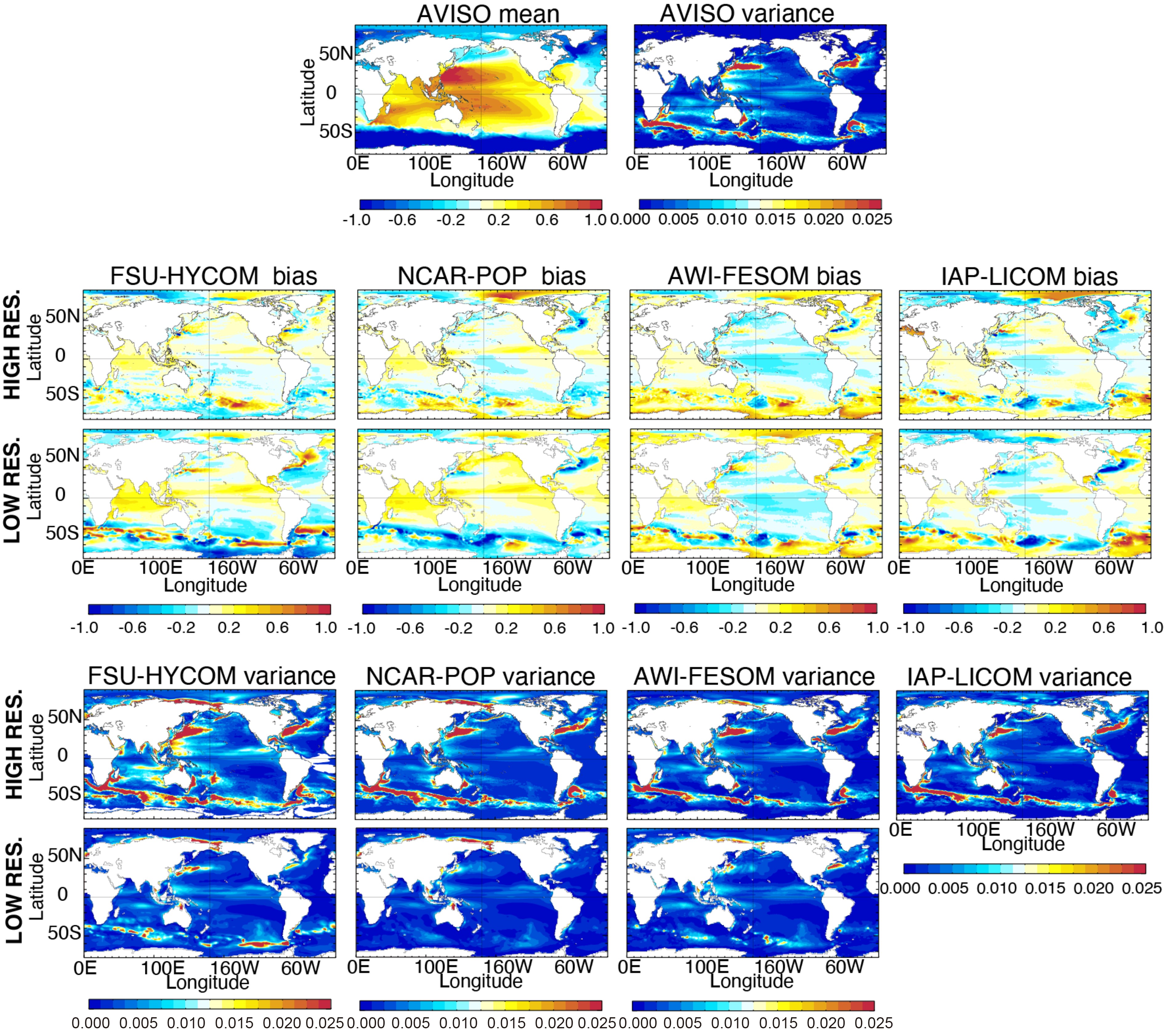Figure2. Top panel: Mean 1993–2018 SSH (units: m) and variance of AVISO. Middle panel: Difference between the mean modeled SSH and AVISO SSH. Bottom panel: Modeled variance derived from five-day average outputs. The low-resolution LICOM SSH variance was not provided. [Reprinted from Chassignet et al. (2020a)].


From a climate perspective, researchers are especially interested in the time evolution of ocean heat content, sea level, and sea ice. The high-resolution models have a tendency to warm up more rapidly at depths below 700 m than the coarse-resolution models. Griffies et al. (2015) did find that vertical heat transport differs depending on if the eddies are parameterized (coarse-resolution) or resolved (high-resolution), and errors in eddy subgrid-scale parameterizations could, therefore, be responsible for this tendency. Overall, despite a significant improvement in the position, strength, and variability of western boundary currents, equatorial currents, and the Antarctic Circumpolar Current, there is no consistent improvement in temperature and salinity drift among the models when the horizontal resolution is increased. Some regions even display increased biases [see Chassignet et al. (2020a) for details]. In summary, an increase in horizontal resolution does not always deliver clear bias improvement everywhere for all models.

A smaller model domain is more computationally affordable and, therefore, allows more in-depth investigation of the impact of horizontal resolution (e.g., Hurlburt and Hogan, 2000; Lévy et al., 2010; Chassignet and Xu, 2017; Schubert et al., 2019). Chassignet and Xu (2017), in a series of North and Equatorial Atlantic simulations, showed that as the resolution is increased to a submesoscale-resolving 1/50° (~1.5 km at midlatitudes) from an eddying 1/12°, the representation of the Gulf Stream penetration and associated recirculating gyres shifts from unrealistic to realistic (see legend of Fig. 3 for details), and the penetration of EKE into the deep ocean is drastically improved and more closely resembles observations [see Figs. 15 and 16 in Chassignet and Xu (2017) for details]. However, they noted several discrepancies between the high-resolution 1/50° numerical simulation and observations. The most notable discrepancies were 1) an area of high surface EKE and/or SSH root-mean-square (RMS) wider than observed near the New England seamounts chain (Figs. 4a, b) and 2) SSH surface power spectra in the 70–250 km mesoscale range independent of latitude (Fig. 8). In the remainder of this section, we will show that the inclusion of high-resolution bathymetry details and tidal forcing has a strong impact on the modeled fields and significantly improve the model’s ability to represent the observed ocean variability.
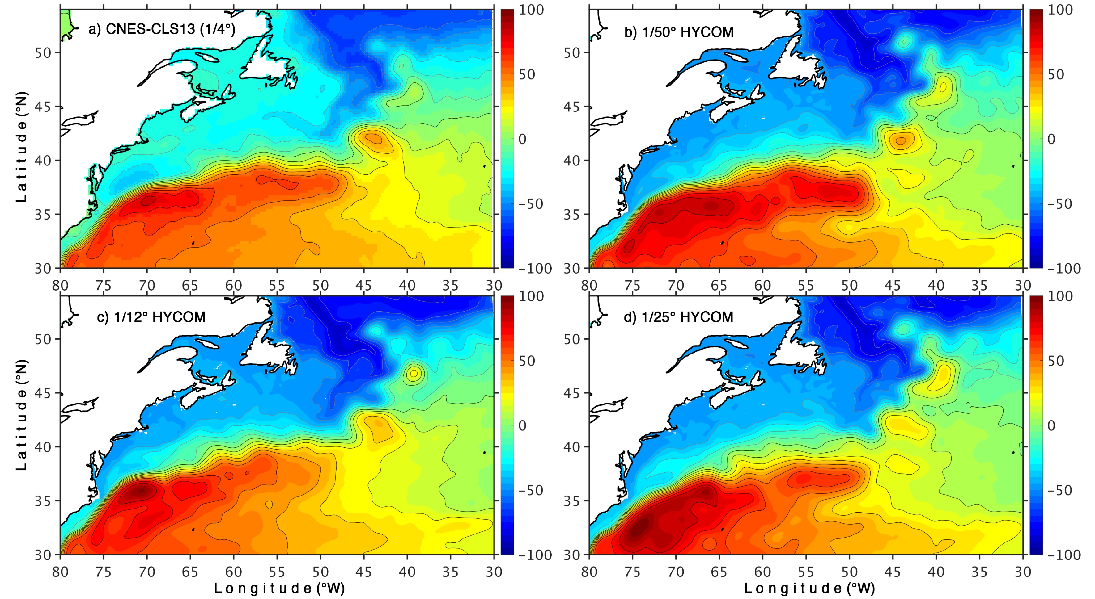Figure3. Mean SSH (units: cm) in the Gulf Stream region: (a) 1993–2012 observed mean from Rio et al. (2014), (b) 1/50°, (c) 1/25°, and (d) 1/12° HYCOM (years 16–20). [Adapted from Chassignet and Xu (2017)]. In the three simulations, the Gulf Stream separates at Cape Hatteras, but the extent of its eastward interior penetration varies greatly. At 1/12° (Fig. 3c), the modeled Gulf Stream does not extend far into the interior and the SSH variability (Fig. 4c) is concentrated west of the New England seamounts (60°W). There is no visible improvement when the resolution is doubled to 1/25° (Fig. 3d) simulation – on the contrary, there is an unrealistically strong recirculating gyre southeast of Cape Hatteras with excessive surface variability (Fig. 4d). On the other hand, when the resolution is increased to 1/50° (Fig. 3b), the Gulf Stream penetration, recirculating gyre, and extension become very realistic and compare extremely well to the latest mean dynamic topography derived from observations (top left panel).


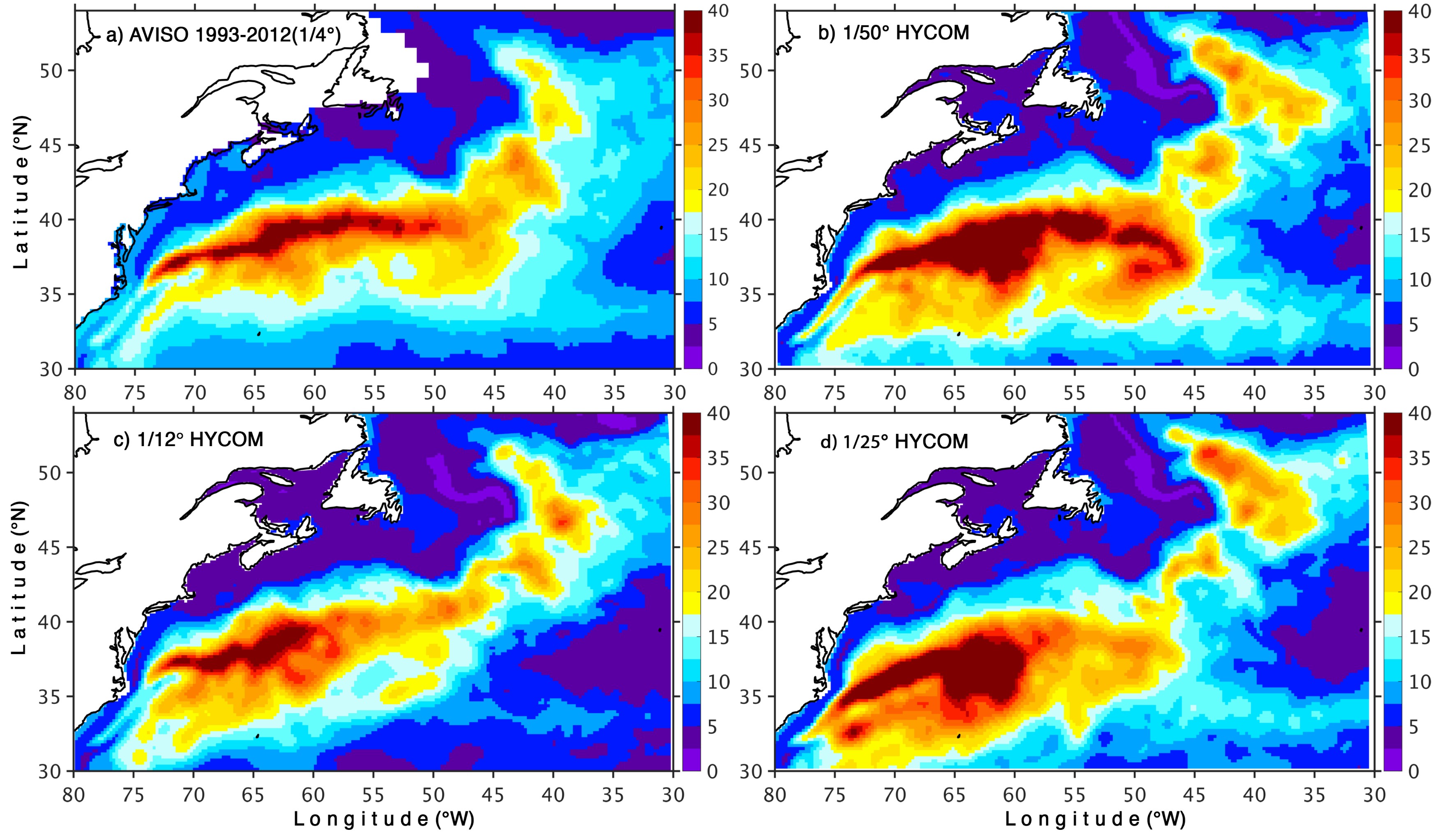Figure4. SSH variability (units: cm) in the Gulf Stream region, (a) based on AVISO (1993–2012) and (b–d) the 1/50°, 1/25°, and 1/12° HYCOM simulations, respectively (years 16–20). The model outputs were filtered to be representative of the AVISO gridded outputs by subsampling of the model outputs to the AVISO 1/4° grid, time averaging the outputs over 10 days, and applying a 150 km band pass filter.



2

-->

4.1. Impact of bathymetry

The fact that the modeled high SSH variability is wider than observed near the New England seamounts chain in the 1/50° experiment (Fig. 4b) suggests that interactions with the topography may be overemphasized in that specific configuration. In this section, we will show that the bathymetry has a much more profound impact on the Gulf Stream pathway than one would have a priori anticipated. In Chassignet and Xu (2017), the goal was to perform a convergence study where most parameters are not changed as the grid spacing is refined from 1/12° to 1/50° and the bathymetry used for the 1/50° configuration (hereafter referred to as NEATL) was linearly interpolated from the coarser 1/12° topography based on the 2’ Naval Research Laboratory (NRL) digital bathymetry database, which combines the global topography based on satellite altimetry of Smith and Sandwell (1997) with several high-resolution regional databases. To investigate the impact of a higher-resolution bathymetry, the last five years of NEATL were repeated (hereafter experiment NEATL-HB) with a new bathymetry derived from the latest 15 arc-seconds GEBCO 2019 bathymetry, which contains significantly higher resolution topographic features (see detailed difference in bathymetry displayed in Fig. 7); all other parameters are identical to those of NEATL (see Chassignet and Xu (2017) for a detailed description).
The five-year mean SSH for NEATL (coarse bathymetry) and NEATL-HB (fine bathymetry) are shown in Fig. 5 together with the latest observational estimate (Rio et al., 2014). Overall, both agree well with the observed mean (Fig. 5a), but there is a significant difference in the Gulf Stream mean pathway between the two simulations when the Gulf Stream crosses over the New England seamounts chain (area highlighted in the bottom two panels of Fig. 5). The SSH contours are much closer to each other and the Gulf Stream pathway is tighter in the high-resolution bathymetry experiment (NEATL-HB) than in the reference experiment (NEATL) with coarse linearly interpolated 1/12° bathymetry. The impact of the bathymetry is further illustrated by and is more striking in the plots of SSH variability for the last five years of both simulations (Fig. 6). Not only is the excess SSH variability near to the New England seamounts chain found in the experiment with coarse bathymetry (NEATL) gone, the shape of the variability and distribution of the variability in the experiment with high-resolution bathymetry is a very close match to the observations. This includes a deflection of the SSH variability to the north near 64°W when the Gulf Stream passes over the New England seamounts chain (see highlight in Figs. 5 and 6).
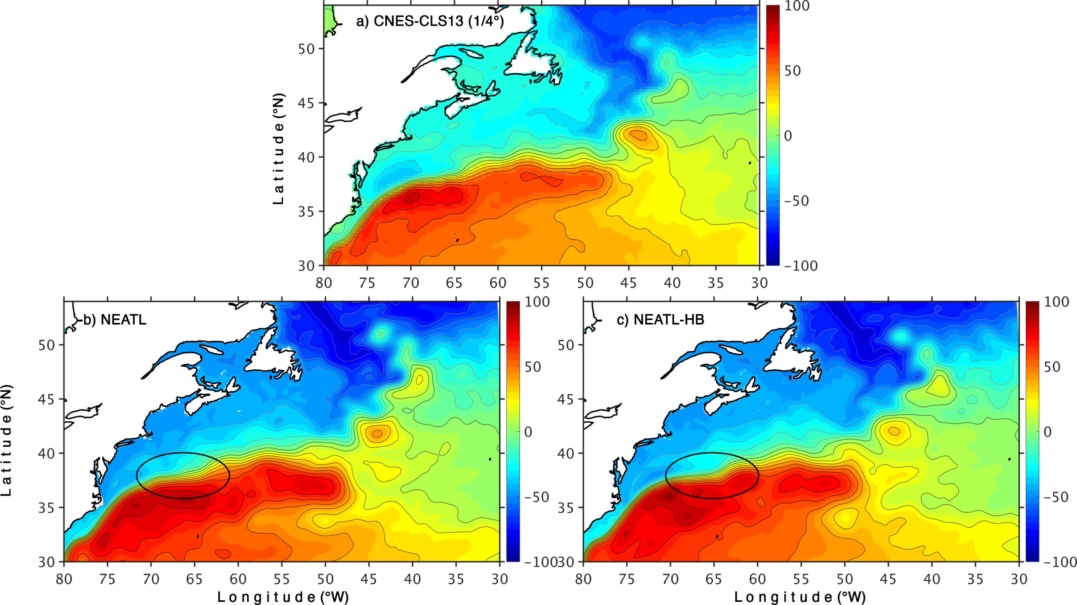Figure5. Mean SSH (units: cm) in the Gulf Stream region for (a) 1993–2012 observed mean from Rio et al. (2014), (b) NEATL, and (c) NEATL-HB (years 16–20).


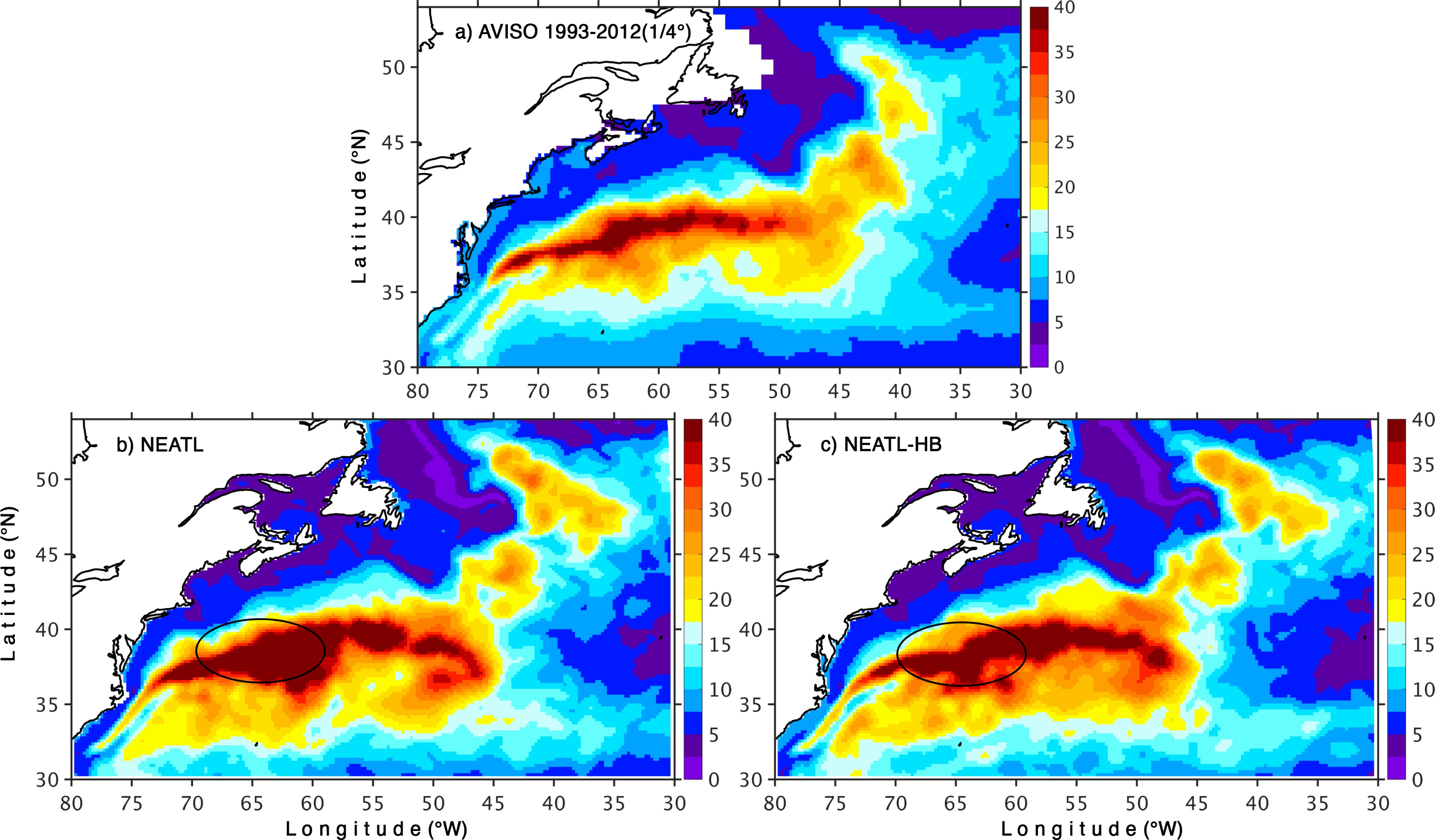Figure6. SSH (units: cm) in the Gulf Stream region for (a) AVISO (1993–2012), (b) NEATL, and (c) NEATL-HB (years 16–20). The model outputs were filtered as in Fig. 4.


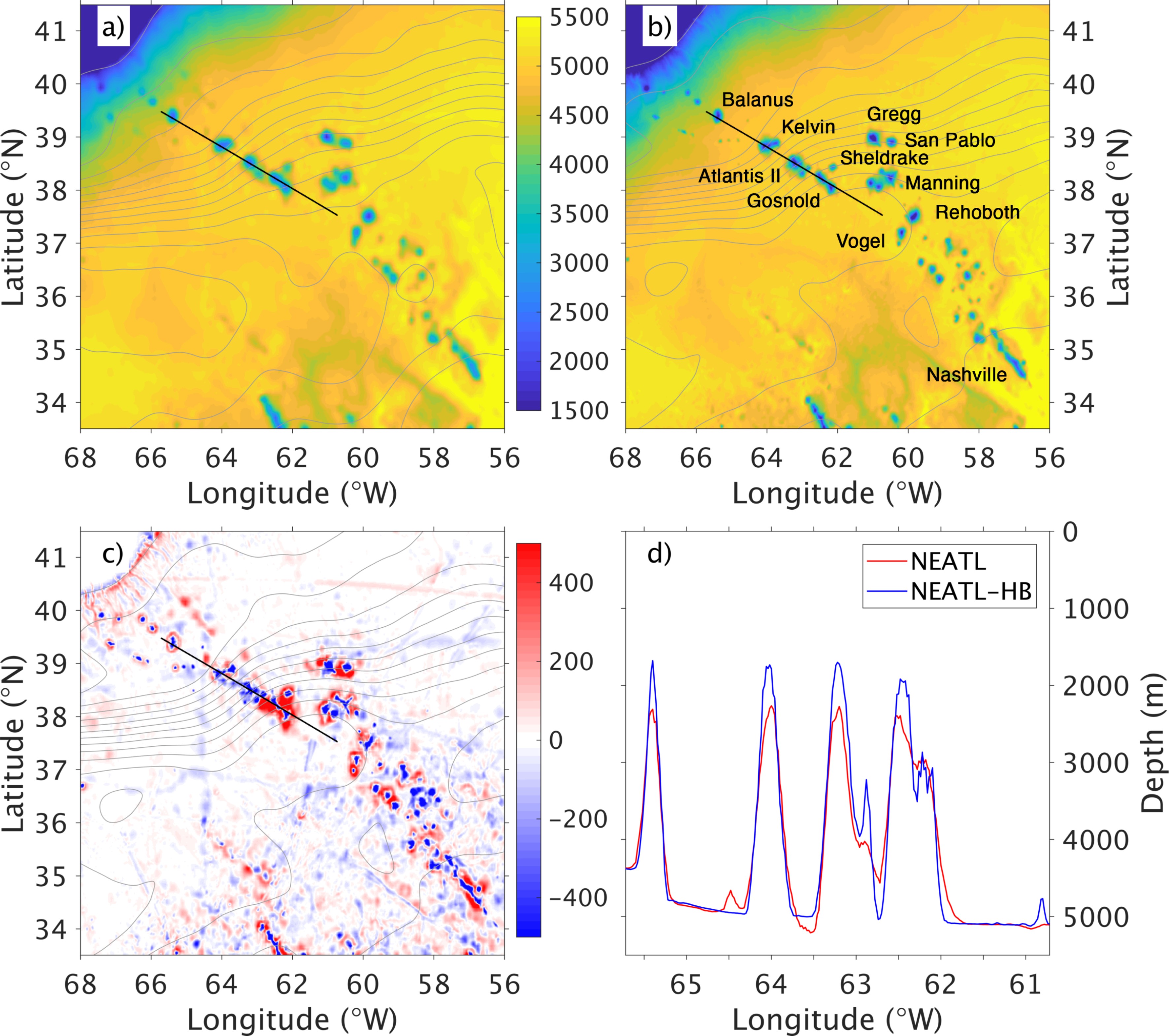Figure7. (a) NEATL bathymetry in meters; (b) NEATL-HB bathymetry in meters with the names of the major seamounts (Houghton et al., 1977); (c) difference in bathymetry in meters between NEATL-HB and NEATL, blue color indicates a shallower depth in NEATL-HB and vice versa. The gray contours are the modeled five-year mean SSH in NEATL-HB indicating the mean Gulf Stream pathway; and (d) bathymetry along the central portion of the New England seamount chain (black line in left panel) that encounters the Gulf Stream direcly. The four seamounts from west to east are Balanus, Kelvin, Atlantis II, and Gosnold.


The difference in bathymetry between the two experiments for the New England seamounts area is shown in Fig. 7c. In many respects, the differences are quite small (less than 100 m in most areas where the depth is close to 5000 m) with the biggest magnitude being around the seamounts. The bathymetry cross-section along the seamount chain (Fig. 7d) shows that the most striking difference is in the height of the seamounts (500 m higher in the water column), which are closer in NEATL-HB to the base of the permanent thermocline of 1000–1500 meters (Meinen and Luther, 2016). But the higher resolution bathymetry also better resolves the spatial extent of the New England seamounts (Figs. 7a and b), making them narrower and effectively increasing the separation distance between them, especially for the seamounts located between 62°W and 63.5°W (i.e., Atlantis II, Shelldrake, and Gosnold, Fig. 7b) and under the southern extent of the Gulf Stream. We interpret the difference in SSH variability between the two experiments, NEATL and NEATL-HB, as follows: In the coarse bathymetry experiment (NEATL), the three seamounts (Atlantis II, Shelldrake, and Gosnold) between 62°W and 63.5°W are not clearly separated from each other, and therefore, as discussed by Zhang and Boyer (1991), they can act as a single body and will appear as a large obstacle to the eastward flowing Gulf Stream. This in turn leads to larger meanders downstream of the seamounts via conservation of potential vorticity (Holton and Hakim, 2012) and consequently higher downstream eddy kinetic energy (Barthel et al., 2017). In the high-resolution bathymetry experiment, there is a larger separation distance between the seamounts, and the resulting flow field past the seamounts is determined by the interaction of the stream with relatively independent narrow obstacles, leading to less downstream variability (Zhang and Boyer, 1991). Thus, the instability processes induced by the Gulf Stream interacting with the New England seamounts are significantly diminished with better resolved topographic features and isolated seamounts. The reduced instabilities lead to a tighter Gulf Stream mean path that agrees better with the observed path and a narrower extent of high surface eddy kinetic energy that is in excellent agreement with the observations.

2 -->

4.2. Impact of tides on the SSH wavenumber spectra

SSH wavenumber spectra are commonly used in the literature to quantify the energy and variability associated with different temporal and spatial scales. In the reference experiment (NEATL), the slope of the surface power spectra in the 70–250 km mesoscale range is mostly independent of latitude and ranges between –5 and –4 (Fig. 8b); it is only slightly flattened near the equator and in the northern North Atlantic near 60°N. However, altimeter observations (Fig. 8a) show large spatial latitudinal variability in the distribution of the SSH wavenumber spectra with steep slopes closer to –5 at midlatitudes and flattened slopes near –1 in the tropics (Xu and Fu, 2011, 2012; Zhou et al., 2015; Dufau et al., 2016). A lack of latitudinal dependence in the 70–250 km band with slopes between –5 and –4 was also found in previous modeling studies (Paiva et al., 1999; Richman et al., 2012, Sasaki and Klein, 2012; Biri et al., 2016), and several explanations have been put forward to explain the differences with the altimeter observations. This includes aliasing and noise in the altimetry data (Biri et al., 2016) and underestimation of the impact of high frequency motions (i.e., internal waves and tides) when using daily averages to compute the wavenumber spectra (Richman et al., 2012; Rocha et al., 2016; Tchilibou et al., 2018). Previous studies (Rocha et al., 2016; Tchilibou et al., 2018) have shown that internal tides can have a significant impact on the wavenumber spectra, especially on small scales. Therefore, we further investigated the latitudinal dependence of the SSH power spectra on high-frequency motions by adding tidal forcing to the 1/50° North and Equatorial Atlantic HYCOM simulation in the last 1.5 years of NEATL (hereafter referred to as NEATL-T-HB). In NEATL-T-HB, eight tidal constituents (M2, S2, O1, K1, N2, P1, K2, and Q1) are added via body and lateral boundary forcing. At the northern and southern boundaries, the phase and amplitude are specified using the TPXO8-atlas global tidal solutions from Oregon State University. All other parameters are identical to that of NEATL (see Chassignet and Xu (2017) for a detailed description).
Figure 8 shows the slope of the SSH wavenumber spectra in the 70–250 km mesoscale range in 10° × 10° boxes over the North Atlantic domain from both NEATL and NEATL-T-HB. The latitudinal dependence is drastically different in NEATL-T-HB from that of the reference experiment with slopes that are close to –1 in the tropics as in the observations (Fig. 8a). This is due to tidal forcing and the generation of internal tides since the addition of high-resolution bathymetry alone was found to have only a very small impact on the slope of SSH power spectra in the 70–250 km mesoscale range (sensitivity experiment not shown). The tidal forcing in NEATL-T-HB generates internal tides that have a strong SSH signature (Fig. 9, bottom panel) that is not present in the absence of tidal forcing (Fig. 9, top panel). These internal tides are generated in areas of strong topography around the Azores, the Cape Verde islands, off the North Brazil coast near the Amazon estuary, as well on the northern side of the Georges Bank past the New England seamounts. The surface signal associated with the internal tides significantly modifies the power spectra in the equatorial region (Fig. 10) with two peaks, one in the 110–130 km range and another one at near 70 km, which flatten the slope in the equatorial region (Fig. 8c). This leads to a modeled spectral slope in the equatorial region that is in excellent agreement with the filtered observational estimate of Zhou et al. (2015) (Figs. 8 and 10). The impact of the internal tides on the power spectra is not as large in the midlatitudes (Fig. 8) because the magnitude of the SSH variability is lower in the equatorial region than in the midlatitudes [see Fig. 26 of Chassignet and Xu (2017) for details].
Figure9. Root-mean-square (RMS) of the high-frequency steric SSH variability (units: cm) for (a) NEATL and (b) NEATL-T-HB. The RMS is calculated daily from 24 hourly snapshots of the steric SSH and is averaged over a month (December) – the results do not change if a longer time average is used.


Figure8. Slope of the SSH power spectra in the 70–250 km mesoscale range in 10° × 10° boxes: (a) observational estimate of Zhou et al. (2015); (b) NEATL, and (c) NEATL-T-HB. Note that the sign of the slope was reversed.


Figure10. SSH power spectra calculated along altimeter tracks and computed as a four 10° × 10° boxes average across the equator (35°–15°W, 10°S–10°N). Red and blue lines are results for year 20 of NEATL and NEATL-T-HB; the black lines are observations (unfiltered and filtered for noise) (Zhou et al. 2015); and the gray line are unfiltered observations (Dufau et al. 2016).

As stated in Chassignet and Xu (2017) and further supported by the additional experiments reported here, it is clear there is substantial improvement in the models’ ability to represent the observed ocean variability and western boundary currents when the horizontal resolution is increased from the eddying 1/10° to submesoscale-enabled 1/50° grid spacing. As stated in Stewart et al. (2017), it is also important to resolve the vertical structure of the ocean currents in accordance to the baroclinic modal decomposition that can be resolved by the horizontal grid. In other words, the finer the grid spacing, the higher the number of vertical modes one can resolve, and consequently, the vertical grid spacing needs to be chosen accordingly in order to properly capture the baroclinic dynamics of a given mode. For the HYCOM experiments reported here, the vertical resolution is lower than what is recommended by Stewart et al. (2017) for z-coordinate models, but the statistics of the eddy scales and the vertical structure of the resolved eddy motions are well captured by the HYCOM layer discretization when compared to a z-coordinate kilometric model with 300 levels (Ajayi et al., 2020, 2021). When trying to isolate the effects of horizontal resolution, one should always strive to only change the horizontal resolution and associated physics.
The considerable differences in surface EKE in the global high-resolution models of Chassignet et al. (2020a) were associated with the use of relative winds versus absolute winds. Chassignet and Xu (2017) showed that the level of EKE in the 1/50° simulation was comparable to the observations when one takes into account the aliasing associated with the altimeter sampling. However, this was obtained by using absolute wind stresses at the ocean surface which do not allow any oceanic feedback to the atmosphere via SST (Small et al., 2008; Ma et al., 2016) or ocean current/wind shear (Renault et al., 2020). The use of relative winds in the wind stress can lead to a significant reduction of the surface EKE (on the order of 30%; Renault et al., 2020). This implies that the next generation of numerical simulations will need to either further increase the horizontal resolution or use less dissipative numerical operators in order be able to reach a level of EKE comparable to observations when using relative winds. In addition, the bulk formulae used in this class of models do not take into account any partial re-energization of the ocean by a changing atmosphere. A parameterization of this effect was recently proposed by Renault et al. (2020), but another approach, short of coupling the ocean model to an active atmosphere (HighResMIP, Haarsma et al., 2016), is to use an intermediate complexity marine atmospheric boundary layer model as in Lemarié et al. (2020) to represent the key processes associated with air–sea interactions on characteristic oceanic scales in the ocean-only numerical simulations.
The computational cost of simulations at 1/50° is extremely large, and while currently available computer resources do not allow for decadal global simulations at that resolution, we will soon have the ability to do so in the future. Ocean/climate modelers are one of the biggest groups of users of computer resources, and as resolution is further refined, they will always require the latest generation of supercomputers. This means that further progress will only take place when the numerical codes used in ocean models take full advantage of the latest computing architecture, and this implies close collaborations with computer scientists. Presently, supercomputer development is closely linked to the performance of commodity chips (i.e., GPUs), and because of their reduced memory access, these are not well-adapted to ocean applications. The main limitation is, therefore, not just the computational speed of the processors but also, as stated by Le Sommer et al. (2018), access to memory and latency in reading/writing on disk drives (see Wang et al. (2020) for an application of a GPU-based version of LICOM3).
Acknowledgements. EPC would like to thank Dr. Hailong LIU and his colleagues for their warm welcome during EPC’s visit in summer 2019 to the State Key Laboratory of Numerical Modeling for Atmospheric Sciences and Geophysical Fluid Dynamics, Institute of Atmospheric Physics, Chinese Academy of Sciences, Beijing, China. Support for this visit was made possible by the Chinese Academy of Sciences (CAS) President's International Fellowship Initiative (PIFI). This overview article is heavily influenced by and reiterates many of the key points found in articles, chapters, and review papers written by the authors. Appropriate references were made, but there are many similarities in content and style to these publications throughout this article.
Open Access This article is distributed under the terms of the Creative Commons Attribution 4.0 International License (http://creativecommons.org/licenses/by/4.0/), which permits unrestricted use, distribution, and reproduction in any medium, provided you give appropriate credit to the original author(s) and the source, provide a link to the Creative Commons license, and indicate if changes were made.