Chao ZHANG¹,
Hailong LIU^2,3,,,
Jinbo XIE²,
Chongyin LI^1,2,
Pengfei LIN^2,3

Corresponding author: Hailong LIU,lhl@lasg.iap.ac.cn;

1.College of Meteorology and Oceanography, National University of Defense Technology, Nanjing 211101, China
2.State Key Laboratory of Numerical Modeling for Atmospheric Sciences and Geophysical Fluid Dynamics, Institute of Atmospheric Physics, Chinese Academy of Sciences, Beijing 100029, China
3.College of Earth and Planetary Sciences, University of Chinese Academy of Sciences, Beijing 100049, China
Manuscript received: 2020-03-24
Manuscript revised: 2020-07-03
Manuscript accepted: 2020-07-17
Abstract:This study examines the artificial influence of increasing the SST resolution on the storm track over the North Pacific in ERA-Interim. Along with the mesoscale oceanic eddies and fronts resolved during the high-resolution-SST period, the low-level storm track strengthens northward, reaching more than 30% of the maximum values in the low-resolution-SST period after removing the influence of ENSO. The mesoscale structure firstly imprints on the marine atmospheric boundary layer, which then leads to changes in turbulent heat flux and near-surface convergence, forcing a secondary circulation into the free atmosphere, strengthening the vertical eddy heat, momentum and specific humidity fluxes, and contributing to the enhancement of the storm track. Results from a high-resolution atmospheric model further indicate the changes in the storm track due to the mesoscale SST and their relationship.
Keywords: storm track,
mesoscale SST,
air?sea interaction,
ERA-Interim,
CAM4
摘要:本文研究了ERA-Interim资料中海温分辨率的提高对北太平洋风暴轴的人为影响。在海温高分辨率时期, 海洋中尺度涡旋和海洋锋能够被更好地识别出来。风暴轴的差异主要表现为向北增强, 相对于低分辨率时期去除ENSO影响后的风暴轴的最大值, 增强了约30%。提高海温分辨率影响风暴轴的机制可以概括为: 在高分辨率时期, 海洋的中尺度结构会影响海气边界层, 导致湍流热通量的改变以及近表层风场的辐合, 从而激发出次级环流。异常的垂直运动不仅仅局限在边界层内, 还会突破边界层影响到自由大气, 并增强了垂直方向上天气尺度涡旋热量、动量及水汽通量。大气中水汽和热量增加, 使得黑潮-亲潮延伸体区域内大气斜压性增强, 有利于通过斜压能量转换过程增强涡旋动能, 从而使得局地风暴轴的强度增强。此外, 本文利用高分辨率模式的试验结果也进一步暗示了中尺度海温可能是引起风暴轴改变的重要原因。
关键词:风暴轴,
中尺度海温,
海气相互作用,
ERA-Interim,
CAM4

HTML

--> --> -->

The European Centre for Medium-Range Weather Forecasts (ECMWF) interim reanalysis (ERA-Interim) dataset is typically applied to detect climate change (Chang and Yau, 2016), assess interannual or decadal variability (O’Reilly and Czaja, 2015; Wills and Thompson, 2018), or evaluate against model results (Piazza et al., 2016; Ma et al., 2017; Lee et al., 2018). However, the prescribed sea surface temperature (SST) resolution for the ERA-Interim analysis system has been increased twice since 1979, resulting in a significant impact on the marine atmospheric boundary layer (MABL) (Masunaga et al., 2015, 2016; Parfitt et al., 2017). Masunaga et al. (2015) noted that mesoscale features, such as surface wind convergence and cloudiness, can only be seen during the period with high-resolution SST. Parfitt et al. (2017) showed the sensitivity to the SST resolution of the frontal air?sea interaction in the Gulf Stream region. The authors found that the occurrence of atmospheric cold fronts and precipitation increased up to 30% during the high-resolution period, along with strengthening of the surface storm track.
The increased spatial resolution of the prescribed SST translates to better resolved mesoscale features of the ocean, especially in some eddy-rich regions such as the Kuroshio Extension area or Gulf Stream area. Different from the large-scale air?sea interaction, the atmosphere is forced by the ocean at the meso scale (Bishop et al., 2017). Recent studies have further suggested the important role of oceanic mesoscale eddies (Ma et al., 2015b, 2017) and fronts (Nakamura et al., 2008; Small et al., 2008; Kuwano-Yoshida and Minobe, 2017) on the storm track. Comparing twin experiments in a regional atmospheric model, one with realistic SST and another with spatial smoothing SST, Ma et al. (2017) showed that removing the mesoscale SST not only led to a reduction in the local storm track intensity, but also forced a significant southward shift in the storm track over the eastern North Pacific. Similar results were also found over the North Atlantic (Piazza et al., 2016). In addition, Woollings et al. (2010) showed that the storm track intensity in the model was overestimated along the coast of North America when the SST resolution was low, which was later confirmed by Small et al. (2014). A recent study by Small et al. (2019b) also pointed out that the storm track location improved in the coupled model with an eddy-resolving ocean model.
According to the aforementioned studies, the mesoscale SST signals resolved by high-resolution SST could play an important role in the intensity and location of the storm track. Therefore, the increases in SST resolution in ERA-Interim may be able to change the storm track characteristics and introduce artificial signals. Meanwhile, the storm track, which is known to serve as a bridge of air?sea interaction at midlatitudes, could greatly influence weather and climate processes. Such an artificial effect would be very likely to introduce uncertainties and mislead us into reaching inaccurate or wrong conclusions. For example, if we ignore this effect, the long-term trend may be overestimated or underestimated, especially considering global warming.
In the present study, we attempt to identify and quantify the signals of the storm track due to the increase in the prescribed SST resolution in ERA-Interim. How does its pattern change due to the increased SST resolution? The results will help us to clarify the uncertainties of the ERA-Interim dataset in terms of both the spatial pattern and temporal variability of the storm track in the North Pacific, as well as benefit studies of climate change.

ERA-Interim is available on a 0.75° grid for the period January 1979 to December 2018 (Dee et al., 2011). We mainly use the daily fields, such as SST, sea level pressure (SLP), horizontal wind, specific humidity, and air temperature. In addition, the surface heat fluxes are taken from the forecasting system. The prescribed SST resolution in ERA-Interim has increased twice, from 1.0° to 0.5° on 1 January 2002, and from 0.5° to 0.05° on 1 February 2009. The SST dataset with a resolution of 0.5° was from NCEP Real-Time Global SST, and then the Operational Sea Surface Temperature and Sea-Ice Analysis (OSTIA) from February 2009 (Dee et al., 2011). Despite the oversampling of the OSTIA product, all of these SST datasets were interpolated to the same model grid, which was the same as the atmospheric model. The latter has remained at the same resolution from 1979 to the present day (ECMWF, 2019). It is also important to note that, except for the SST datasets, the atmospheric physical processes do not change. Here, the period of January 1979 to December 2001 is referred to as the low-resolution (LR) period, while the period of February 2009 to December 2018 is the high-resolution (HR) period. Although the prescribed horizontal resolution of ERA-Interim is 0.75°, Masunaga et al. (2015) suggested that mesoscale features were well represented during the ERA-Interim HR period, and were overall consistent with high-resolution satellite observations (see their Fig. 1).
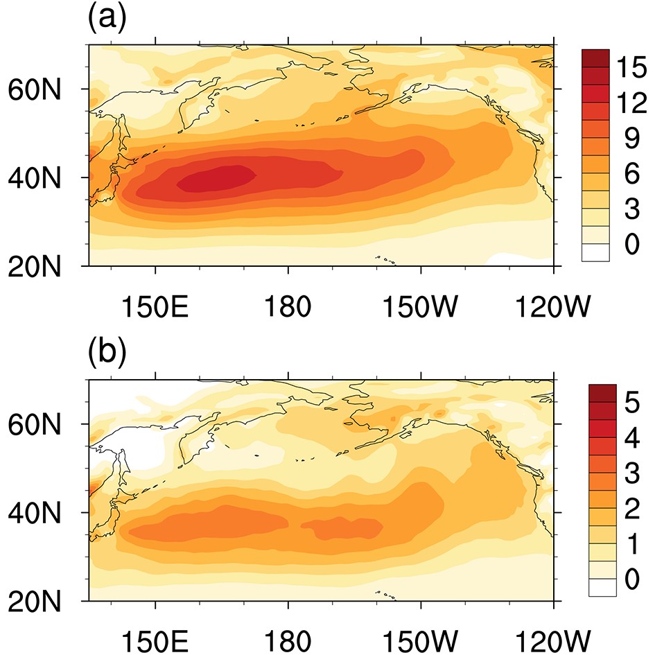Figure1. (a) Winter-mean storm track measured by the meridional eddy heat flux (v′T′; units: m s^?1 K) in the LR period. (b) As in (a) but for the storm track with the influence of ENSO linearly removed.


To separate the mesoscale signals, a 5° × 5° spatial boxcar filter was employed (Small et al., 2019a; Zhang et al., 2019). First, we calculated the area average in the 5° × 5° box for the original field (X) at every grid point. Then, the smoothed field was obtained, referred to as <X>. Next, the mesoscale anomalies (X^*) were defined as the original field minus the smoothed one. This procedure is denoted as a high-pass boxcar filter and can be expressed as X^* = X ? <X>, where < > represents the low-pass spatial filter. We examined our boxcar filter carefully and compared it with other methods, such as the Loess spatial filter used in Ma et al. (2017). The results demonstrated that the mesoscale signals with wavelength less than 500 km could be well separated by this boxcar filter (not shown).
The storm track in the present study is represented by the meridional eddy heat flux ($v'T'$; Nakamura et al., 2002; Taguchi et al., 2009; Yao et al., 2018), the synoptic-scale variance in meridional wind ($v^\prime v^\prime $; Hoskins and Hodges, 2002), and eddy kinetic energy at 850 hPa. The prime here denotes the synoptic-scale eddies, which were derived by a 2?8-day Lanczos bandpass filter (Duchon, 1979). The focus of this paper is on midlatitude air?sea interaction, and so the influence of ENSO on the storm track was reduced by the removal of the linear regression on the Ni?o3.4 index (Qiu et al., 2014; Small et al., 2019b). This process can be expressed as follows:
where $X(t)$ is the atmospheric variable, ${X_{\rm{e}}}(t)$ is the ENSO signal, and ${X_{\rm{n}}}(t)$ stands for the part not influenced by ENSO. N, α, and b are the Ni?o3.4 series, regression coefficient, and residual, respectively. Czaja and Frankignoul (2002) showed that the covariance between the atmosphere and SST anomalies reached a maximum after two months in the observation, indicating that the atmospheric response may take a few months to fully develop (Ferreira and Frankignoul, 2005). Following previous studies (Frankignoul et al., 2011; Gan and Wu, 2013; Révelard et al., 2016), two-month lagged regression was applied (τ = 2). Figure 1 shows an example of the storm track before and after linearly removing the ENSO impacts.
To identify the response to the increase in SST resolution in ERA-Interim, we directly computed the difference in the climatological winter mean variables between the HR and LR periods (HR minus LR). To avoid the influences of interannual variabilities in the LR period, the differences were further computed following the method of Parfitt et al. (2017), in which the winter means of the randomly selected eight years during the LR period were also used, denoted as “LRi”, where “i” is the identifier of the different samples. Here, 1000 random samples during the LR period were selected to compute the differences. The average (AVE) and standard deviation (STD) of these differences can be used to measure the effects of the SST resolution and the interannual variability, respectively.
Two simulations using the high-resolution Community Atmosphere Model, version 4 (CAM4; Neale et al., 2013) were conducted to further confirm the impact of mesoscale SST on the storm track: one with the eddy-resolving prescribed SST, and the other with the smoothed SST, referred to as the control run (CTRL) and mesoscale-SST-filtered run (MSFR), respectively. In MSFR, the mesoscale SST was filtered out by the low-pass spatial boxcar filter with scales of 5° × 5°. CAM4 was configured on the finite-volume dynamical core with an approximately 25-km horizontal resolution and 26 vertical levels. A five-year integration with the “present-day” greenhouse gas conditions and the monthly climatological SST boundary condition (climatological mean around 2000) was first conducted as a spin-up run. The results of the final day of the spin-up integration were then used as the initial condition of CTRL and MSFR. Meanwhile, the SST boundary condition was taken from a high-resolution coupled model output with a horizontal resolution of 0.1° × 0.1° (Lin et al., 2019). As the horizontal resolution of the daily SST is higher than that of CAM4, it was then interpolated to the CAM4 grid based on the areal conservative remapping method. Next, the remapped daily SST was used to force the atmospheric model. The two simulations were run for six model-years.

2

-->

3.1. Changes in SST and its impact on the storm track

Figure 2a shows the differences in the climatological winter mean SST between the HR and LR periods, which shows significant positive and negative anomalies across the Kuroshio and Oyashio confluence region (KOCR; 33°?45°N, 142°?175°E), where the oceanic mesoscale eddies are active (Chelton et al., 2011). The maximum and minimum of the differences over KOCR are 1.96°C and ?1.93°C, respectively, while the positive and negative anomalies over the eastern North Pacific between 180°E and 130°W can only reach values of about 0.91°C and ?0.66°C.
Figure2. (a) Differences (colors; unit: °C) in the wintertime climatology of the SST between the HR and LR periods (HR minus LR) and the climatological SST (CI = 3°C, CI means contour interval.) during the HR period. (b) Average (colors; unit: °C) and STD (CI = 0.05°C) of the differences between the HR and LRi periods. (c) Climatological mesoscale SST (unit: °C) during the HR period. (d) As in (c) but for the LR period. The red box defines the KOCR.


The average of the differences between the HR and each LRi period is shown in Fig. 2b, which is similar to that in Fig. 1a, with the pattern correlation coefficient reaching 0.99 for the whole region. In addition, the maximum and minimum of the mean values (shaded) over KOCR are 2.01°C and ?1.93°C, which are also very close to those in Fig. 2a. This result indicates that the pattern of SST differences is barely affected by the period we selected during LR, and the effects of interannual variability in the LR period are negligible.
The contours in Fig. 2b show the STD of the differences between the HR and LRi periods. The large values occur in KOCR, indicating a relatively strong natural variability there. Moreover, the value of the maximum STD is only 0.32°C, which is less than the values of the differences in Fig. 2a (maximum of 1.96°C). This result confirms the robustness of the differences against interannual variability. The results of more random samples also show a similar pattern (not shown).
To separate the mesoscale SST, we applied the high-pass 5° × 5° spatial boxcar filter mentioned above to the SST field in both the LR and HR periods, the results of which are shown in Figs. 2c and d, respectively. The high-pass-filtered SST anomalies are confined within KOCR, while anomalies of SST over the eastern North Pacific disappear. The pattern of SST differences in KOCR in Fig. 2a is similar to the mesoscale SST during the HR period (Fig. 2c), with the pattern correlation coefficient reaching 0.71. The maximum and minimum of mesoscale SST during the HR period are 1.90°C and ?1.83°C, respectively—only slightly less than the SST differences between the HR and LR period. However, there is almost no mesoscale signal in the high-pass-filtered SST during the LR period (Fig. 2d), with the positive and negative values reaching 0.58°C and ?0.67°C in KOCR, respectively. Therefore, we speculate that the SST differences between the HR and LR period over KOCR arose from the increase in the SST horizontal resolution and are mainly dominated by mesoscale SST, while the anomalies in the eastern North Pacific are at a large scale and probably induced by the climate variabilities between the HR and LR periods, such as the Pacific Decadal Oscillation and global warming.
Compared to that of the LR period, the pattern of the storm track during the HR period, measured by the meridional eddy heat flux ($v^\prime T^\prime $) at 850 hPa, shows a northward strengthening. The differences of the storm track show an enhancement over KOCR and extend northeast to the Aleutian Islands (Fig. 3a), while it decreases over the northwestern North Pacific as well as the Gulf of Alaska. The maximum and minimum of the differences in the meridional eddy heat flux are 1.16 m s^?1 K and ?1.12 m s^?1 K, respectively, while the maximum of the climatological mean storm track (ENSO influence linearly removed) is 2.95 m s^?1 K, nearly 30%?40% of the maximum climatology. In addition, the maximum and minimum of the AVE values (shaded) over the North Pacific are 1.15 m s^?1 K and ?1.12 m s^?1 K, which are very close to those in Fig. 3a. However, the value of the maximum STD is 0.93 m s^?1 K, which is comparable to the AVE maximum. This result suggests a subtle influence of the increased SST resolution on the low-level storm track.
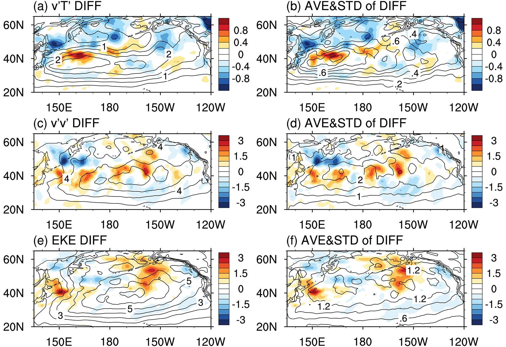Figure3. (a) Differences (colors; units: m s^?1 K) of the wintertime climatology of the storm track represented by the meridional eddy heat flux ($v^\prime T^\prime $) at 850 hPa between the HR and LR periods; the contours represent the climatology of the storm track during the LR period (CI = 0.5 m s^?1 K). (b) Average (colors; units: m s^?1 K) and STD (contours; CI = 0.1 m s^?1 K) of the differences between the HR and LRi periods. (c, d) As in (a, b) but for synoptic-scale variance of meridional wind ($v^\prime v^\prime $) at 850 hPa [colors; units: m² s^?2; CI = 2 m² s^?2 in (c) and CI = 0.5 m² s^?2 in (d)]. (e, f) As in (a, b) but for EKE at 850 hPa [colors; units: m² s^?2; CI = 1 m² s^?2 in (e) and CI = 0.3 m² s^?2 in (f)].


The differences of other storm-track metrics, such as the variance of meridional eddy wind ($v^\prime v^\prime $) and eddy kinetic energy [EKE=$(u^{\prime 2} + v^{\prime 2})/2$], between the HR and LR periods were also investigated (Figs. 3c-f). The changes of $v^\prime v^\prime $ resemble the pattern of $v^\prime T^\prime $ in Fig. 3a, but with a broader positive-anomaly band showing the storm track strengthening across KOCR and in the downstream region. The pattern of the differences barely changes in the AVE (Fig. 3d), indicating a robustness of the difference in the storm track between the HR and LR periods. Although the pattern of EKE differences seems to differ little with that in Figs. 3a and c, it also shows an enhancement near Japan and a positive anomaly to the north of the climatology of EKE near the Gulf of Alaska in the LR period. Besides, we examined the response of the high-level storm track, which was measured by the variance of meridional eddy wind at 300 hPa (not shown). It showed a similar pattern as that at 850 hPa, indicating a deep and significant effect of SST anomalies in the troposphere. These results agree with previous studies revealed by Chen et al. (2019) and Tao et al. (2019). Therefore, the response of the storm track can be independent from the metrics. Particularly, it should be noted that the method used to calculate the difference could not fully remove the influence of decadal climate variability.

2 -->

3.2. Local response

Masunaga et al. (2015) suggested that the mesoscale SST anomalies could imprint on the MABL. Figure 4 shows the mesoscale SST and surface heat flux differences between the HR and LR periods. The turbulent heat flux anomalies (Fig. 4c), defined as the sum of latent heat flux and sensible heat flux, are in phase with the mesoscale SST anomalies, with the pattern correlation coefficient reaching 0.89 over KOCR. Indeed, the changes of turbulent heat flux are dominated by the latent heat flux, accounting for more than 50% over KOCR (Fig. 4). This result suggests that more (less) heat fluxes out of the ocean over the warm (cold) mesoscale SST anomalies. Small et al. (2019a) revealed that, in midlatitude ocean frontal zones, the variability of surface heat fluxes is driven by small-scale SST on monthly time scales. The ocean forcing of heat flux further leads to the changes in the MABL thermal structure, represented by the in-phase variation of the meridional SST gradient and surface temperature gradient, with the pattern correlation coefficient reaching 0.88 (Fig. 4d). Changes can then be found in near-surface convergence/divergence, as described below.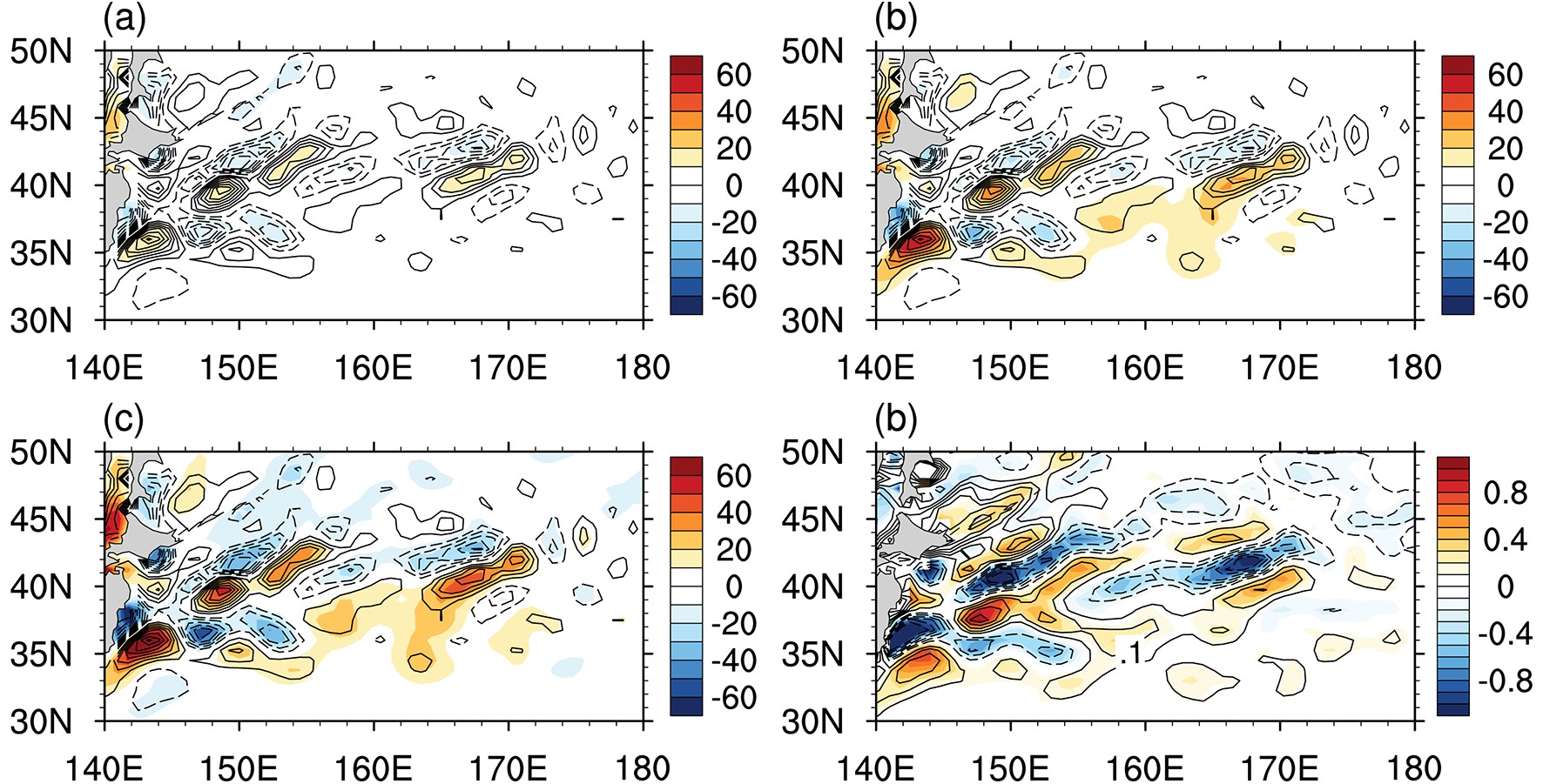
Figure4. Differences (colors) between the HR and LR periods for (a) sensible heat flux (units: W m^?2), (b) latent heat flux (units: W m^?2), (c) turbulent heat flux (units: W m^?2), and (d) meridional SST gradient [colors; units: °C (100 km)^?1]. Contours represent mesoscale SST (CI = 0.2°C) in (a?c) and the meridional air temperature gradient [CI = 0.05°C (100 km)^?1] in (d). For clarity, the zero contour is omitted in all plots.


Two mechanisms are usually applied to explain the local atmospheric response to frontal-scale or mesoscale SST. One is the “pressure adjustment mechanism” (PAM; Lindzen and Nigam, 1987), which suggests in-phase spatial coherence among the sign-reversed SST Laplacian, the Laplacian of SLP, and near-surface wind convergence. Minobe et al. (2008) showed that the wind speed convergence is proportional to the SLP Laplacian as follows:
where ${\rho _0}$, u, v, P and f are the air density, zonal wind, meridional wind, SLP, and Coriolis parameters, respectively. $\varepsilon $ is the constant damping coefficient, and its value is 2.0 × 10^?4 s^?1 (Takatama et al., 2012; Piazza et al., 2016). Across KOCR, the spatial pattern of the SLP Laplacian difference between the HR and LR periods is close to that of the SST Laplacian, with the pattern correlation coefficient reaching ?0.62 (Fig. 5a). Meanwhile, there is a high resemblance between the SLP Laplacian and wind convergence (correlation coefficient of 0.67; Fig. 5b). The significant correlation among them indicates that the PAM is operative.
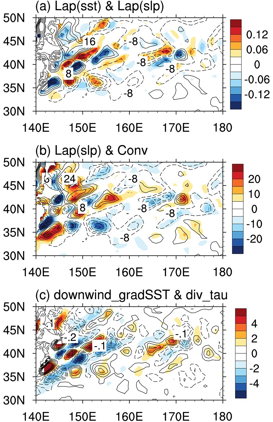Figure5. Differences (colors) between the HR and LR periods for (a) the Laplacian of SST (units: 10^?7 K m^?2), (b) near-surface convergence (units: 10^?7 s^?1), and (c) the downwind SST gradient [units: 10^?6°C (100 km)^?1]. The contours represent the Laplacian of SLP (CI = 8 × 10^?7 Pa m^?2) in (a, b) and wind stress divergence (CI = 0.1 N m^?3) in (c). For clarity, the zero contour is omitted in all plots.


The other mechanism is vertical momentum mixing (VMM; Wallace et al., 1989), which attributes the changes of surface wind speed to atmospheric instability. The strength can be measured by the linear relationship between wind stress divergence and downwind SST gradients (Ma et al., 2015a; Piazza et al., 2016). Figure 5c shows the differences of downwind SST gradients and wind stress divergence. Here, the downwind SST gradient is calculated by ${{k}} \cdot \nabla {\rm{SST}} = ({{V}}/\left| { {{V}} } \right|) \cdot \nabla {\rm{SST}}$, where V is the 10-m wind vector and k the wind direction. As shown, the shape of the downwind SST gradient is very similar to the wind stress divergence, with a correlation coefficient of 0.79, which demonstrates the VMM. In fact, the relative contributions of the two mechanisms has long been debated (Small et al., 2008). Using a high-resolution atmospheric general circulation model, Koseki and Watanabe (2010) suggested that these two mechanisms make almost equal contributions in the Kuroshio Extension in January. In contrast, the results reported by Chen et al. (2017) showed VMM to be dominant, occupying 60% in the winter Kuroshio Extension region. On the other hand, considering the different atmospheric background wind direction, Schneider and Qiu (2015) and Bai et al. (2019) indicated that the response to SST in the MABL is quietly different, suggesting that the relative importance of PAM and VMM should be studied under different wind conditions.
The imprints on the MABL suggest that the improved prescribed SST resolution does exert a significant influence on the near-surface atmosphere. But how does the impact penetrate into the free atmosphere and force the storm track in the troposphere? Figure 6a plots the cross-section of vertical motion and convergence at pressure levels along 42°N, and Fig. 6c shows the profiles of the SLP Laplacian and mesoscale SST at the same latitude. It is clear that an upward (downward) motion is induced over the convergence (divergence), forcing a secondary circulation above the oceanic eddies. Moreover, the vertical velocity anomalies are not confined within the MABL and could penetrate into the free atmosphere (above 700 hPa). Also, Fig. 6a implies that the VMM can be operative since the convergence and divergence patches straddle the peaks of high-pass-filtered SST.
Figure6. (a) Longitude?pressure section along 42°N of differences in vertical velocity (colors; positive upward; units: 10^?2 Pa s^?1) and convergence (CI = 5 × 10^?7 s^?1) at pressure levels. The magenta and green lines denote the boundary layer height during the HR and LR periods, respectively. (b) As in (a) but for differences in vertical eddy heat flux ($\omega ^\prime T^\prime $; colors; units: 10^?2 Pa K s^?1), vertical eddy momentum flux ($\omega ^\prime v^\prime $; gray contours; CI = 2 × 10^?2 Pa m s^?2) and vertical eddy specific humidity flux ($\omega ^\prime q^\prime $; purple contours; CI = 4 × 10^?6 Pa s^?1 kg kg^?1). (c) The black and red lines denote the mesoscale SST anomalies (unit: °C) and Laplacian SLP (units: 10^?7 Pa m^?2) along 42°N, respectively. (d) Differences in the baroclinic energy conversion of the eddy available potential energy to EKE (colors; units: W m^?2) and the storm track measured by EKE (CI = 0.5 m² s^?1) at 850 hPa between the HR and LR periods. For clarity, the zero contour is omitted in (a, d).


As a consequence, the vertical eddy fluxes strengthen over KOCR (Fig. 6b). Cai et al. (2007) suggested that the vertical eddy heat flux is closely related with the baroclinic conversion (BC) between the eddy available potential energy and EKE, which is expressed as follows:
where ω is vertical velocity and ${C_1} = {({P_0}/P)^{{C_v}/{C_p}}}(R/g)$. R and C_p (C_v) represent the gas constant for dry air and the specific heat capacity of dry air at constant pressure (volume), respectively. Figure 6d shows the difference in BC at 850 hPa between the HR and LR periods. The positive anomaly east of Japan further indicates the strengthening of the storm track during the HR period. Besides, the enhancement of vertical eddy specific humidity flux over KOCR, which is associated with latent heat fluxes, can also significantly wetten the atmosphere. As shown in Ma et al. (2017), the moist atmosphere could reduce the static stability and strengthen the baroclinicity in the atmosphere, ultimately leading to the enhanced storm track.

2 -->

3.3. Response of the storm track in model results

Due to the method for calculating the differences in the storm track, changes may be induced by both the influence of the increase in SST resolution and/or the long-term climate variability between the HR and LR periods, most likely on the decadal time scale. As shown in Fig. 2, increasing the SST resolution results in the differences dominating at the meso scale over KOCR. To investigate the role of mesoscale SST in the storm track and to exclude the effects of the climate variability on the decadal time scale, we conducted two experiments using a high-resolution model, CAM4. One was forced by the eddy-resolving prescribed SST and the other by the smoothed SST, denoted as CTRL and MSFR, respectively. The potential differences between the two simulations suggest the influence of mesoscale SST without the long-term climate variability. However, these mesoscale SSTs may be induced by oceanic eddies and fronts. To determine the components of these mesoscale SSTs, the meridional SST gradient was then calculated to represent the oceanic fronts. The climatological mean SST gradient magnitudes for the two simulations were averaged within KOCR to provide a single representative value. The magnitude of the oceanic front decreased only 4% in MSFR compared to that in CTRL. We suspect that the mesoscale structure of the differences in the SST in our case may be mainly induced by the oceanic eddies, rather than the SST front. The influence of SST fronts is beyond the scope of this paper, but is worthy of further investigation in the future.
Therefore, the response of the storm track to mesoscale SST was examined. Similarly, the influence of ENSO on the storm track was removed. Here, the ENSO signal is defined by the first principal component of monthly SST anomalies in the tropical Pacific between 12.5°N and 12.5°S. Figure 7e shows the differences of winter mean SST in CTRL and MSFR. Across KOCR, the mesoscale SST anomalies dominate, which agrees with the situation during the HR period in ERA-Interim (Fig. 2c). The differences of meridional eddy heat flux between CTRL and MSFR show that the storm track is significantly enhanced across KOCR (Fig. 7f). Moreover, the positive anomalies extend northeast from KOCR to the Gulf of Alaska, while the negative anomalies occur over the eastern and northwestern North Pacific, which shows a similar pattern to the differences in Figs. 3a and c. These results further indicate that the differences in the storm track between the HR and LR periods can be induced by the increase in the prescribed SST resolution in ERA-Interim. However, it should be noted that the specific location and value of the response are not closely consistent with the observation. This may be explained by the fact that the climatology of the storm track in the model is not identical to that in the observation. Also, the shorter period of model results may be another contributory factor for the inconsistency.
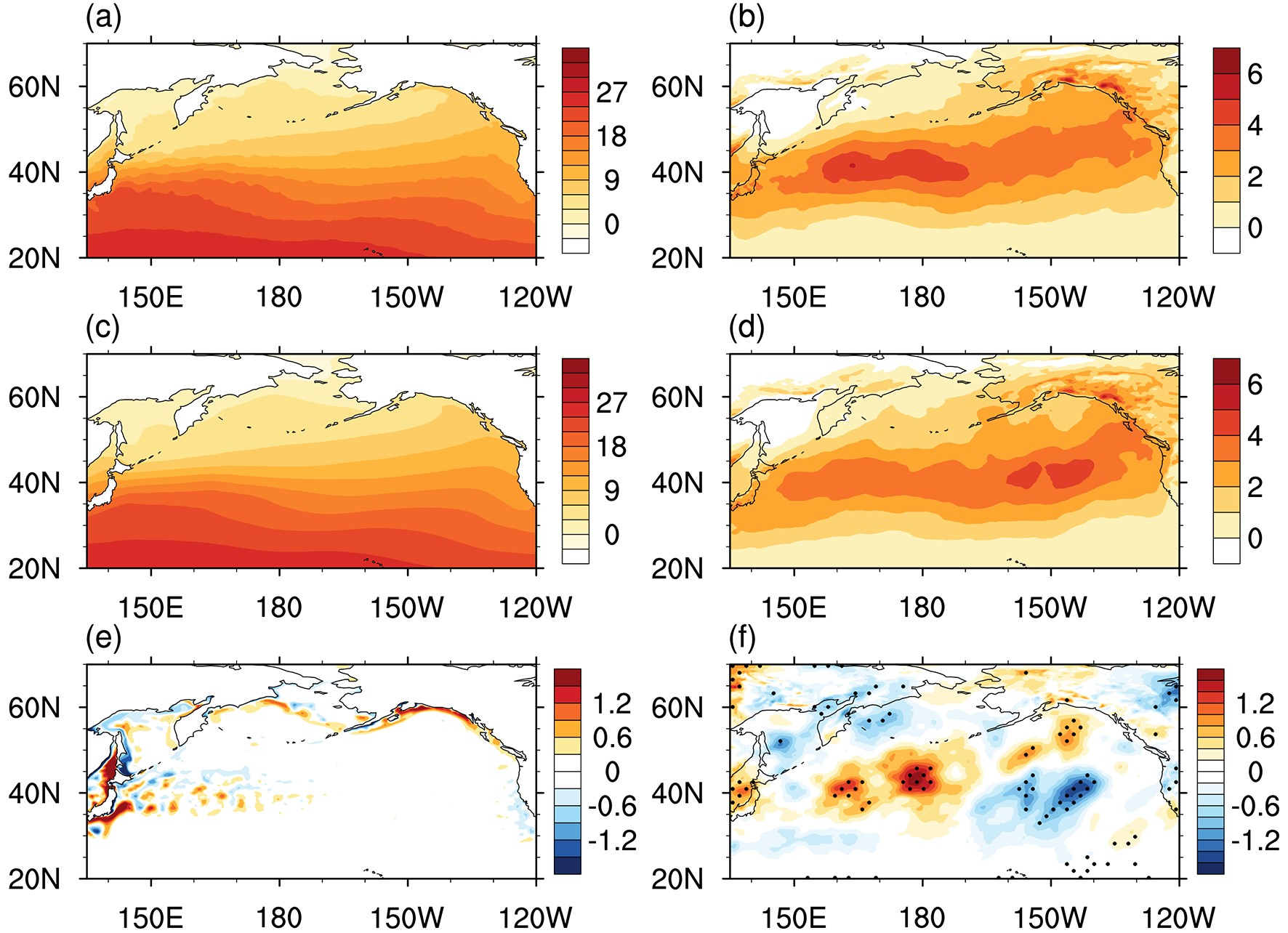Figure7. (a) Winter mean SST (unit: °C) in CTRL. (c) Winter mean SST (units: °C) in MSFR. (e) Differences (colors) of SST between CTRL and MSFR, with the winter mean of SST in MSFR overlaid. (b, d, f) As in (a, c, e) but for the storm track represented by the transient eddy heat flux at 850 hPa (units: m s^?1 K). Statistically significant differences at the 95% confidence level according to the bootstrapping test are stippled.


To quantify the magnitude of the changes in storm track, a metric following Small et al. (2014) is introduced, $M = \max |\overline {{S_{{\rm{HR}}}} - {S_{{\rm{LR}}}}} |/\max (\overline {{S_{{\rm{LR}}}}}) \times 100$ (unit: %), which is expressed as the percentage of the maximum absolute difference between the HR and LR periods to the maximum value of the storm track during the LR period. The S and (ˉ) stand for the variables representing the storm track and the temporal mean during winter. The M is calculated over the domain of the North Pacific (30°?60°N, 140°?240°E). The M value of the meridional eddy heat flux and the variance of the synoptic-scale meridional wind is 39% and 32%, respectively. Then, we calculated the value of M for CAM4, which was roughly 42% of the maximum value in MSFR.

This study investigated the artificial changes of storm track induced by the increase in the SST resolution in the ERA-Interim dataset over the North Pacific. Along with the signals of resolved mesoscale oceanic eddies and fronts, the storm track strengthens northward across KOCR during the HR period. The positive anomalies of meridional eddy heat flux or meridional momentum flux extend from east of Japan to the northeastern North Pacific. The differences of storm track between the HR and LR periods reach more than 30%?40% of the maximum values during the LR period after removing the influence of ENSO. In addition, a set of experiments using a high-resolution atmospheric model were used to further examine whether the changes of the North Pacific storm track can be due to the resolved mesoscale SST. The results also indicated that the changes in SST horizontal resolution possibly affect the long-term variability amplitude of the storm track. Therefore, the artificial influence induced by the changes in SST resolution should be considered when analyzing the long-term variability using the ERA-Interim dataset.
The mechanism by which the mesoscale SST impacts the storm track can be summarized as follows. The mesoscale imprints were first found in the turbulent heat flux with more (less) heat fluxed out of the ocean over the warm (cold) SST. That will further change the thermal structure in the MABL, and lead to anomalous convergence/divergence at the surface, forcing a secondary circulation above the mesoscale SST anomalies over KOCR. The PAM and VMM are both operative to the response of near-surface convergence. However, our results from reanalysis data could not fully separate the respective contributions of the PAM and VMM. The impact can penetrate into the free atmosphere, enhance the vertical eddy heat, momentum and specific humidity fluxes, and finally strengthen the storm track intensity in the free atmosphere both locally and remotely.
Note also there is a large-scale positive anomaly of SST in the subtropical North Pacific. Wang et al. (2017) showed that when there is a North Pacific Gyre Oscillation–like positive SST anomaly in the subtropical North Pacific, the intensity of the subarctic frontal zone (SAFZ) gets stronger. This stronger SAFZ tends to lead a northward shift of the baroclinic zone and westerly jet, which also indicates the northward strengthening of the storm track. Recently, studies have also revealed that an intensified subtropical frontal zone (STFZ) would lead to stronger transient eddy activity (Wang et al., 2017, 2019; Chen et al., 2019; Wen et al., 2020). The impact of the STFZ on the intensity of the storm track seems comparable with that to the SAFZ (Yao et al., 2016; Wang et al., 2019). Hence, the relative contribution of the STFZ to the storm track should also be studied in the future. Indeed, based on our model experiments, we have confirmed that only the mesoscale SST anomalies can lead to a similar pattern of changes in the storm track, which indicates that the influences of large-scale SST anomalies may not be as important as the mesoscale SST in this case. Besides, the numerical experiments of Sun et al. (2018) also illustrated that oceanic stochastic forcing due to small-scale SST variability is crucial to the atmospheric circulation above, which can organize well the atmospheric transient eddies and improve the simulated storm track.
In addition, the differences shown in the model experiments might be due to internal climate variability. Furthermore, the atmosphere is highly chaotic and variable in the midlatitudes, and our limited samples may not be sufficient to capture the internal climate variability. However, previous studies have highlighted oceanic mesoscale structures other than internal climate variability that result in changes of the storm track. Ma et al. (2017) conducted twin ensemble simulations using a regional model, each of which contained 10 members. Their results also showed a similar result to ours. They found a significant weakening of the storm track across KOCR after removing the mesoscale SST, indicating a robust influence of mesoscale SST on the atmosphere rather than the climate variability (see their Fig. 5a). In addition, more ensemble simulations using an atmospheric model coupled with a slab-ocean model indicated the ocean mesoscale feedback to the enhancement of the storm track (Jia et al., 2019). Small et al. (2019b) also demonstrated the important role of ocean mesoscale structures on the extratropical storm track using a global coupled model. Based on these valuable works, we focused mainly on the impact of mesoscale SST. Nevertheless, we are planning to investigate the effect of model internal variability in our future work.
Overall, our analysis and experiments, to some extent, show evidence and an indication that the changes in storm track can be due to the resolved mesoscale SST. However, more experiments are needed to prove that part of the changes in the period mean pattern and the climate variability in the ERA-Interim dataset between LR and HR can be attributed to the resolved ocean mesoscale eddies.
Acknowledgements. This study was supported by National Key R&D Program for Developing Basic Sciences (2018YFA0605703, 2016YFC1401401), the National Natural Science Foundation of China (Grant Nos. 41490642, 41776030, 41806034, 4160501) and the research project of the National University of Defense Technology (ZK20-45 and ZK17-02-010). HL and PL acknowledge the technical support from the National Key Scientific and Technological Infrastructure project “Earth System Science Numerical Simulator Facility” (EarthLab). The ERA-Interim data were obtained from the ECMWF at http://apps.ecmwf.int/datasets/data/interim-full-daily/.