HTML
--> --> -->Due to the natural limitations of the Arctic environment, in-situ observations of melt ponds have always been lacking. The melt pond area fraction (MPF) and albedo are the key variables that require observation. During the Surface Heat Budget of the Arctic Ocean Project (SHEBA), the albedo of melt ponds was measured for seven months from April through October and was found to change rapidly in the range of 0.1?0.65 over this time span (Perovich et al., 2002). This variation is closely related to the temporal evolution of melt ponds. Based on observations, Eicken et al. (2004) pointed out that there are generally four stages in melt pond evolution: 1) stage of melt pond formation, 2) stage of meltwater drainage, 3) stage of melt pond stable expansion, 4) stage of melt pond refreezing. These stages are characterized by different mechanisms. Remote sensing provides a new method to collect data for melt pond observation. In 2012, R?sel et al. (2012) used the Moderate Resolution Imaging Spectroradiometer (MODIS) reflectance data to retrieve MPF and provided a data source from May to September 2000?11. Ding et al. (2020) developed a new MPF dataset from 2000 to 2019 based on a deep neural network using MODIS surface reflectance. This new dataset showed great potential for future applications in model parameter estimation and data assimilation for its higher accuracy compared with previously published data. In recent years, microwave remote sensing has been used to observe melt ponds (Scharien et al., 2014; Han et al., 2016; Tanaka et al., 2016), these works demonstrated the potential to produce high-resolution melt pond observations but there are no available products yet. Both field and satellite observations show that the melt pond processes have an obvious spatio-temporal variability. This characteristic needs to be considered in the melt pond parameterization schemes in sea ice models.
The parameterization of melt ponds in sea ice models is a very important research topic. Due to the variations of melt ponds in time and space, directly specifying a fixed albedo for certain types of ice surfaces may cause large simulation errors (Perovich et al., 2002). To calculate a more realistic albedo in sea ice models, it is necessary to develop a melt pond scheme and incorporate it into the sea ice models. Melt pond observation is the foundation for the development of melt pond schemes. There are several melt pond schemes of different complexity. Early-stage melt pond schemes consist of one-dimensional models or two-dimensional models (Taylor and Feltham, 2004; Lüthje et al., 2006; Scott and Feltham, 2010). However, these early schemes fail to align with the sea ice models in use and cannot be incorporated into them.
Holland et al. (2012) proposed a simple melt pond scheme. This scheme can calculate melt pond volume, melt pond fraction, and depth based on a given pond aspect ratio parameter, which is defined as the ratio between average melt pond depth and melt pond area fraction of a model grid cell. The scheme is adopted in the Los Alamos sea ice model (CICE) as the CESM (Community Earth System Model) parameterization scheme. A more complex melt pond scheme was developed directly based on an ice thickness distribution function (ITD) in sea ice models (Flocco and Feltham, 2007; Flocco et al., 2010). The ice surface topography is determined according to ice thickness. The influence of the ice surface topography on the horizontal transport of meltwater is also considered along with the percolation drainage through the permeable ice. This scheme was incorporated into the CICE model as the topography scheme. Hunke et al. (2013) developed the level ice scheme. Based on level ice tracers in CICE, melt ponds are only allowed to exist on level ice. The change of melt pond volume is separated into area and depth, similar to the CESM scheme.
However, these melt pond parameterization schemes are based on several assumptions and include parameters with large uncertainty. Using inappropriate parameters can potentially downgrade the accuracy and reliability of the sea ice models (Polashenski et al., 2012). Generally, sensitivity analysis is often used to study and reduce the uncertainty of these parameters, but in the case of a large number of interdependent parameters, the computational cost of this method is huge and can be prohibitive. The adjoint model provides another possibility for parameter estimation (Kim et al., 2006; Fenty et al., 2017). The adjoint model is the adjoint of the tangent linear model of the original forward model. The derivative of the model output with respect to all model input, including boundary conditions, initial conditions, and model parameters could be obtained through an integration of the adjoint model. Thus, the parameters are estimated quantitatively and efficiently. Adjoint models have been widely used in model parameter estimation and initial condition estimation. For instance, Liu and Zhang (2018) used the MITgcm (Massachusetts Institute of Technology general circulation model) sea ice-ocean coupled model and its adjoint model to study the optimization of the initial condition of sea ice fraction in the sea ice model. The estimated sea ice concentration is closer to the observation than the simulation using the unadjusted initial condition. This result indicates that the adjoint model can be used in the adjustment of the initial field of sea ice models. Fenty et al. (2017) used the MITgcm model and its adjoint model to estimate the coupled sea ice-ocean state for 2004, by assimilating ocean hydrological data and sea ice concentration data. Both the ocean and ice state estimations are more accurate compared to the estimations without assimilation. Kim et al. (2006) used the CICE model and its adjoint model to make a sensitivity analysis of 21 thermodynamic and dynamic parameters in the model. The sensitivities are later used to carry out an estimation of the parameters. This work explores the application of the adjoint model in sea ice model parameter estimation and optimization. The aforementioned research indicates that the adjoint model is useful in parameter estimation of sea ice models, yet melt pond parameters are not considered in these studies. Due to the importance of melt pond to sea ice modeling and existing parameter uncertainty in melt pond schemes, it is interesting to use the adjoint model to estimate and optimize the key melt pond parameters. Implementation of this method should reduce the simulation errors of melt ponds in sea ice models.
In this study, an adjoint model for a melt pond scheme in the CICE6.0 is developed, and the parameters in the melt pond scheme are estimated. The CESM scheme is chosen because of its simplicity in terms of the physical process which is well-suited for adjoint model development. In section 2, the CICE6.0 sea ice model, CESM melt pond parameterization scheme, the adjoint model is developed, and the L-BFGS (Limited-memory Broyden-Fletcher-Goldfard-Shanno) minimization algorithm (Liu and Nocedal, 1989), and datasets are described. Section 3 introduces the verification of the melt pond parameter estimation algorithm and analyzes the parameter estimation results of Arctic sea ice. Section 4 presents the main conclusions and discusses the limitations of our research.
2.1. Observation of melt pond fraction, sea ice concentration, and sea ice thickness
The MODIS MPF data (R?sel et al., 2012) is used as an observational constraint for the parameter estimation, which is provided by the Integrated Climate Data Center, University of Hamburg. The time range spans the warm season, 9 May to 6 September, from 2000 to 2011, with an interval of eight days. The spatial range is 180°W?180°E, 60°?90°N, with a spatial resolution of 12.5 km. The root mean square error (RMSE) of MODIS MPF is in the range of 3.8% to 11.2% compared to the in-situ validation data. MODIS is an optical sensor and could be affected by clouds. There are missing values north of 80°N in 2000, 2001, 2002, and 2007. Missing areas smaller than 12.5 km2 have been interpolated before the release of the data, but areas larger than 12.5 km2 have not been interpolated (R?sel and Kaleschke, 2012). The years with many missing values are avoided and 2005 is chosen for our parameter estimation using an adjoint model.The sea ice concentration data used here is HadISST1 from the Met Office Hadley Centre (Rayner et al., 2003) for its accessibility and the convenience of data processing. HadISST1 integrates sea ice data from historical and satellite observations, providing global monthly sea ice concentrations with a spatial resolution of 1° × 1° since 1871. The sea ice thickness data used is based on upward-looking sonar observations collected by U.S. Navy submarines (Rothrock et al., 2008).
2
2.2. Atmospheric forcing
The JRA55-do data in 2005 derived from Japan Meteorological Agency (JMA) reanalysis JRA-55 is used as the atmospheric forcing data (Tsujino et al., 2018). This dataset is one of the default forcing datasets of CICE6.0. The data includes 10-m air temperature, 10-m specific humidity, 10-m wind velocity, downwelling shortwave flux, downwelling longwave flux, and precipitation with a temporal resolution of three hours. The variables are interpolated to a one-hour time step when used to force CICE6.0.2
2.3. Sea ice model CICE6.0 and melt pond parameterization scheme
In this study, the current version of the Los Alamos sea ice model, CICE6.0 is applied to simulate sea ice conditions at one point (Craig et al., 2018). CICE6.0 is a large-scale thermodynamic-dynamic model based on an ice thickness distribution function (Thorndike et al., 1975). It incorporates the parameterization of sub-grid mechanisms like sea ice ridging (Rothrock, 1975). The North Pole is displaced to land to avoid the singularity problem in computation. As a submodule of CICE6.0, the ICEPACK calculates the vertical sea ice physical and biogeochemical processes (Hunke et al., 2018). The ICEPACK updates the ice temperature by calculating the energy budget of the atmosphere-ice boundary layer and the ice-ocean boundary layer, and then determines the rate of ice growth or melting. CICE6.0 provides a separate driver routine to run the ICEPACK alone to simulate the sea ice state and its change at a single point. In this research, ICEPACK is used in estimating the melt pond parameter for both MYI and FYI.3
2.3.1. CESM melt pond parameterization scheme
The CESM melt pond scheme is one of the three parameterization schemes in CICE6.0, which is slightly different from the one developed in Holland et al. (2012). It calculates the area fraction and depth of melt ponds. The key point of this scheme is an assumed linear relationship between the pond depth and pond fraction,Here,


where


Here


Here


Once

Here

This is physically reasonable because the melt pond on such thin sea ice will be lost to the ocean immediately.
The pond fraction and pond depth calculated here are later used in the calculation of albedo in the shortwave radiation scheme of the sea ice model, thus affecting the absorption of the radiation in the model and playing an important role in the sea ice simulation.
2
2.4. Melt pond adjoint model and its verification
An adjoint model of the melt pond scheme is developed to estimate the pond aspect ratio as a parameter. To develop an adjoint model for an existing model, the first method is to find the analytic equations of the forward model and then derive the corresponding adjoint equations. An adjoint model is the discretization of these adjoint equations. The second method is more straightforward. It is to translate the source code of the forecast model to its adjoint code under the guidance of several rules. This process can be aided by automatic differential software tools (Utke et al., 2008). Automatic differential tools are designed to generate the adjoint model code automatically and are suitable for models developed with the concept of the adjoint in mind, such as the MITgcm. Because forward models are often too complex to isolate their analytic equations, the second method is more commonly used, with or without the aid of automatic differential tools. We adopt the second method, i.e., straightforward line-by-line code transformation to develop the adjoint code without using automatic differential tools. This is because CICE6.0 is complex and is not optimized in code structure for the automatic generation of the adjoint model.The default value of the pond aspect ratio parameter in the CESM scheme is based on an empirical relation derived from the SHEBA observation for FYI. However, the Arctic sea ice is a mixture of MYI and FYI. Melt ponds on rough MYI tend to grow in the vertical direction rather than only in the horizontal direction. This is significantly different from the shallow and wide-spread ponds on flat FYI. Observations show that the MPF is closely related to the type of sea ice (Polashenski et al., 2012; Wang et al., 2017). Typically, the MPF on MYI is lower than that on FYI. The MPF on level FYI can be greater than 0.7, while the MPF on MYI is often lower than 0.4 (Perovich and Polashenski, 2012). Consequently, the pond aspect ratio parameter should be different for MYI and FYI. Therefore, it is necessary to develop an adjoint model of the melt pond scheme to estimate the aspect ratio parameter with the intent of finding a more suitable value.
The steps of developing the adjoint model are as follows. First, the input and output variables of the melt pond scheme are determined. The pond aspect ratio parameter


The correctness of the tangent linear model and adjoint model must be checked before their application. When a perturbation is sufficiently small, the perturbation of the model output from the tangent linear model integration should be very close to that calculated from the forward model integration. Accordingly, the following equation is used to check the correctness of the tangent linear model code:
where Q represents the forward model, z is the input variable vector of Q, and h is a perturbation added to the input variable. P is the tangent linear model,


where P represents the tangent linear model. The


The tangent linear model is checked following Eq. (8). The settings of the scale factor


| Case | $\alpha $ | h |
| 1 | 1.0 | 0.2 |
| 2 | 0.9 | 0.2 |
| 3 | 0.8 | 0.2 |
| 4 | 0.7 | 0.2 |
| 5 | 0.6 | 0.2 |
| 6 | 0.5 | 0.2 |
| 7 | 0.4 | 0.2 |
| 8 | 0.3 | 0.2 |
| 9 | 0.2 | 0.2 |
| 10 | 0.1 | 0.2 |
Table1. The setup of the correctness check of the tangent linear model and adjoint model.

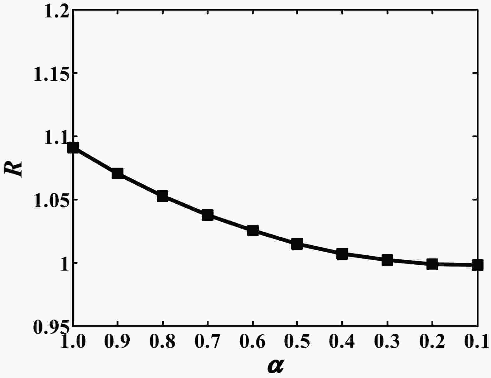 Figure1. Correctness check of CESM melt pond scheme tangent linear model.
The adjoint model is checked following Eq. (9). Here


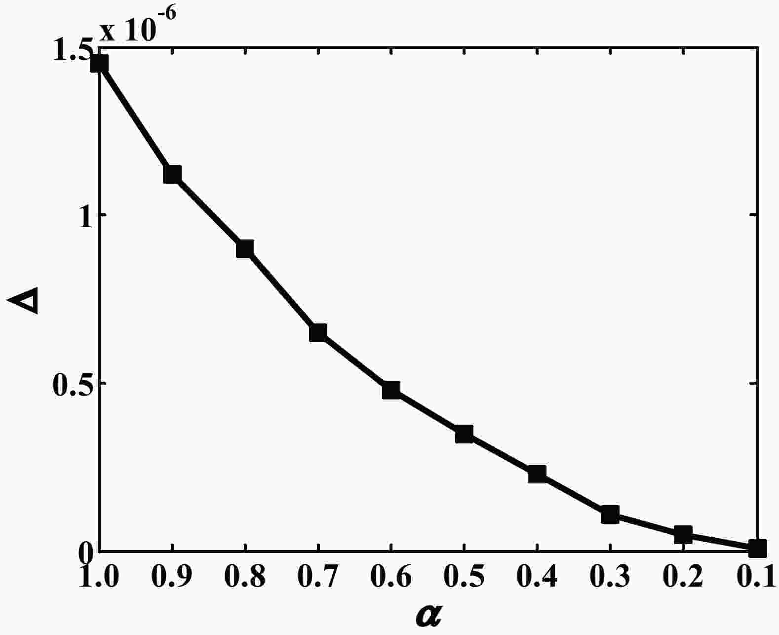 Figure2. Correctness check of CESM melt pond scheme adjoint model.
2
2.5. Parameter estimation and L-BFGS scheme
32.5.1. Parameter estimation algorithm
To estimate the melt pond scheme parameter, an effective algorithm is constructed. The framework of the algorithm is designed as follows. The workflow of the parameter estimation algorithm is shown in Fig. 3. Step 1, a first-guess value of the parameter is set. Step 2, the forward model is integrated to acquire and save the basic state of the pond. At the same time, the melt pond intermediate forcing is saved to drive the melt pond adjoint model at a later time. Step 3, the cost function is calculated according to Eq. (11) using the MPF from the model and observations. Step 4, the adjoint model is integrated under the intermediate melt pond forcing data to acquire the trajectory of the adjoint state variable. Step 5, the gradient of the cost function is calculated. Step 6, the calculated cost function and gradient are sent to the L-BFGS minimization algorithm. The minimization algorithm then automatically adjusts the step size, updates the estimated value of the parameter, and determines whether the specified termination conditions of the iteration are satisfied. If the termination conditions are satisfied, the program will be terminated and return the final estimation of the parameter. Otherwise, the latest estimated value of the parameter will be used as input for step 2 to start a new iteration cycle. When the difference of the estimated parameters from two consecutive iterations is less than a tolerance constant of 10?16 or the norm of cost function gradient


 Figure3. Flow chart of the melt pond parameter estimation algorithm.
3
2.5.2. L-BFGS minimalization algorithm
The parameter estimation could be accomplished by combing the forward model, the adjoint model, and a minimization algorithm. The L-BFGS minimization algorithm is used in our melt pond scheme parameter estimation. It is a quasi-Newtonian method and is widely used in large-scale optimization problems (Liu and Nocedal, 1989). The algorithm updates the parameters according to the following formula:where


Since we aim to estimate the melt pond aspect ratio, the cost function is set as:
Here J is the cost function,


3.1. Melt pond parameter estimation algorithm verification
To verify the parameter estimation algorithm, an ideal experiment method is adopted similarly to previous work (Cao et al., 2011). In the ideal experiment, a forward model integration is carried out using a given parameter and the output of MPF from the forward model is saved as “observation” data. Then the “observation” data is used as the observational constraint of the parameter estimation algorithm. The given pond aspect ratio parameter δp value of 0.8 is the default value used in CICE6.0. The first-guess of the parameter is set to be 0.6. The verification is aimed to examine whether the parameter estimation algorithm can obtain a value of 0.8.The program terminates after seven iterations. The estimated value of the parameter is 0.8. As shown in Fig. 4a, after five iterations, the estimated value of the parameter is already very close to the given value of 0.8. Figure 4b shows the change of cost function J in iterations. The cost function quickly descends to zero after 3 iterations. Figure 4c is the change of norm of the cost function gradient


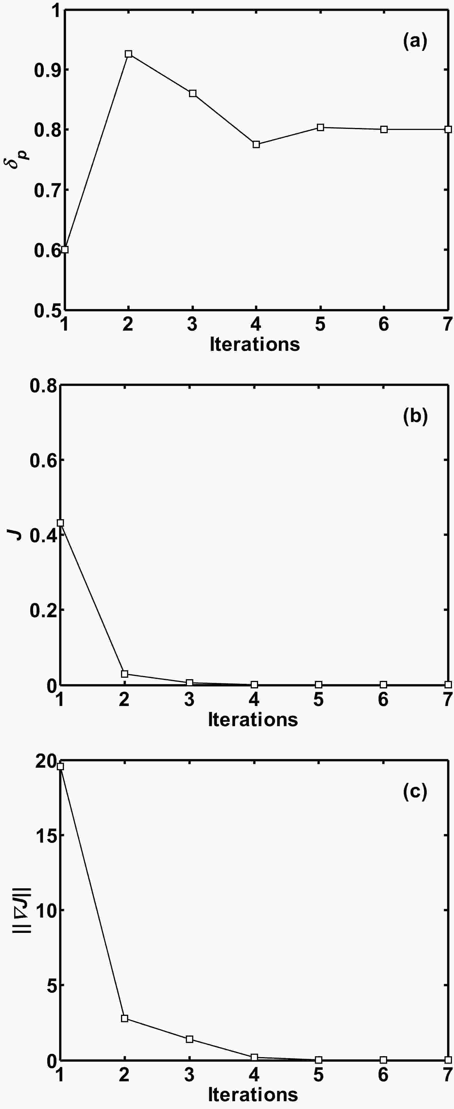 Figure4. Evolution of the (a) the pond aspect ratio parameter, (b) cost function, and (c) norm of cost function gradient with iteration number in the parameter estimation process.
A series of numeric experiments are carried out to examine the influence of the first-guess on parameter estimation results. The result is shown in Table 2, indicating that under different first-guess values, the “correct” parameter estimation of 0.8 can be obtained by the parameter estimation algorithm. Meanwhile, the iteration number in each experiment is less than 10. This shows that the algorithm has high computational efficiency. The above calculation verifies the melt pond adjoint model and parameter estimation algorithm. The results show that they are both correct and effective.
| Case | Given ${\delta _{\rm{p}}}$ | First-guess ${\delta _{\rm{p}}}$ | Estimated ${\delta _{\rm{p}}}$ | Iteration number |
| 1 | 0.8 | 0.1 | 0.8 | 8 |
| 2 | 0.8 | 0.2 | 0.8 | 7 |
| 3 | 0.8 | 0.3 | 0.8 | 9 |
| 4 | 0.8 | 0.4 | 0.8 | 8 |
| 5 | 0.8 | 0.5 | 0.8 | 6 |
| 6 | 0.8 | 0.6 | 0.8 | 7 |
| 7 | 0.8 | 0.7 | 0.8 | 5 |
| 8 | 0.8 | 0.9 | 0.8 | 7 |
| 9 | 0.8 | 1.0 | 0.8 | 7 |
Table2. Results of melt pond parameter estimation under different first-guess values.
2
3.2. Parameter estimation in Arctic regions
33.2.1. Regions
In this section, the parameter estimation is conducted in representative regions of MYI and FYI, respectively. Based on the HadISST1 sea ice concentration data, the MYI region is identified as the region that is covered by sea ice from March to September, while FYI is the region that is covered by sea ice in March and becomes ice-free in September. Figure 5 is the spatial distribution of monthly sea ice concentration in March and September of 2005. The loss of sea ice is most serious in September in the Arctic marginal sea with little to no ice left north of Russia. MODIS data has missing values due to cloud and fog. So, we choose to analyze regions that have fewer missing values to avoid this disadvantage. For the parameter estimation in the later section, the MYI region is chosen to be north of the Canadian Arctic Archipelago (120°W, 80°N). The FYI region is chosen to be in the Kara Sea (90°E, 78°N). The MYI region has one missing time point out of 16 time points while the FYI region has three missing time points out of 16 time points.3
3.2.2. Parameter estimation periods
During the evolution of melt ponds, the change of pond area fraction and pond depth are not synchronous (Eicken et al., 2002). In the first stage of the melt pond evolution, pond fraction increases quickly and the pond aspect ratio remains small; in the second stage, the loss of meltwater from the bottom of sea ice increases and results in a greater pond aspect ratio. In the third stage, the moderately rising pond coverage and stable pond depth reduce the pond aspect ratio. Therefore, for different stages of pond evolution, different pond aspect ratio parameters should be used in the melt pond scheme.Starting from 9 May and ending 6 September, the summertime MODIS observations are divided into 15 periods with each period containing eight days. The parameter is estimated in each period. The MODIS observations are interpolated to a 1-hour interval before parameter estimation for comparison with model output. After interpolation, no missing value is left in the 1-hour MODIS MPF data. The cost function is then defined as the discrepancy between the 1-hour simulation and observations. In the model integration, for each period, we first estimate the melt pond parameter and use it in simulation. Then the simulation outputs at the end of current period are used as the initial condition for the forward model integration of next period. The process of parameter estimation is introduced in section 2.5 and Fig. 3. The MODIS observation is used to constrain the optimization.
3
3.2.3. Model configuration
The integration time of the model is from 1 January 2005 to 1 January 2016 with a time step of 3600 seconds. The Bitz-Lipscomb scheme (Bitz and Lipscomb, 1999), Delta-Eddington scheme (Briegleb and Light, 2007), and CESM scheme are selected as the parameterization schemes for the thermodynamic, short-wave radiation, and melt ponds. Other parameters are set to the default values in the CICE6.0 model. CICE6.0 adopts an ice thickness distribution function to describe the sub-grid scale variation of sea ice thickness. The ice thickness distribution used here has five thickness categories shown in Table 3. HadISST1 sea ice concentration data and US army submarine ice thickness data are used to establish initial conditions. The initial sea ice concentration of MYI is set to 100% according to the nearest HadISST1 data and the initial average ice thickness is set to 2.79 m according to the nearest submarine data, while they are 100% and 1.80 m for FYI. The initial MPF and melt pond depth for both MYI and FYI are 0% and 0 m, respectively.| Category | Lower bound (m) | Upper bound (m) |
| 1 | 0.00 | 0.60 |
| 2 | 0.60 | 1.40 |
| 3 | 1.40 | 2.40 |
| 4 | 2.40 | 3.60 |
| 5 | 3.60 | 5.00 |
Table3. Setup of the ice thickness distribution in experiments.
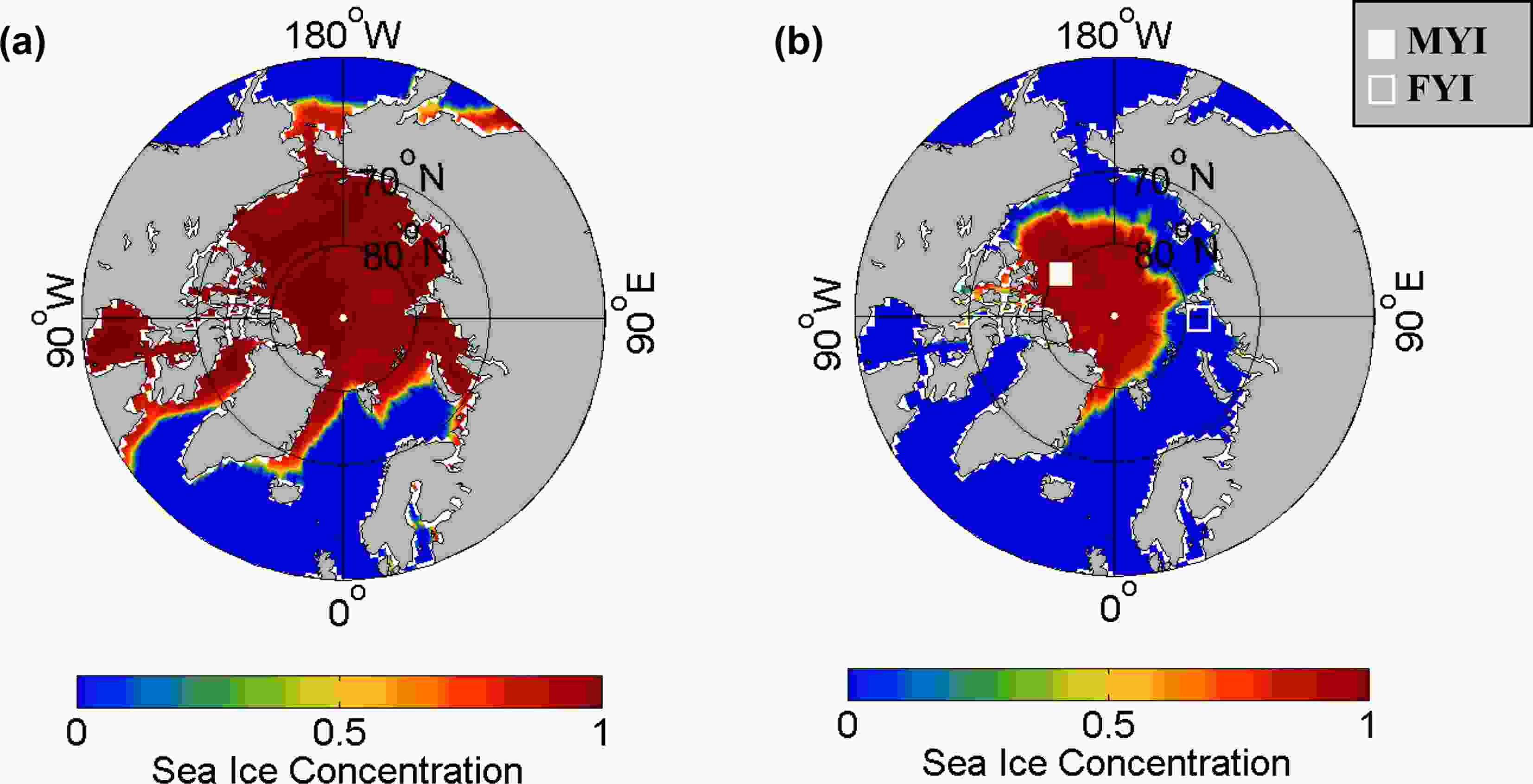 Figure5. Sea ice concentration of (a) March 2005 and (b) September 2005. The white-filled square in (b) represents the MYI study region and the white hollow square represents the FYI study region.
3
3.2.4. Parameter estimation for multi-year ice region
Figure 6a presents the estimated values of the pond aspect ratio parameter for the MYI region. This estimated parameter has a large temporal variation. At the early stage of the melting season, from 9 May to 2 June, the parameter value is relatively large. From 2 June to 26 June, the parameter value drops to around 1. From 26 June to 29 August, the parameter value further, and profoundly, drops to below 0.05. From 29 August to 6 September, the parameter value rises to the default value of 0.8. Overall, the estimated parameter on the MYI region has a descending trend during the melting season. At the early stage of melt pond development, i.e., from 9 May to 26 June, even though there is a large difference in the estimated and default aspect ratio, the simulations of MPF and depth have only minor differences (Figs. 6b and 6c). At this stage, the melt pond volume is small and the simulation difference is also minor. In contrast, from 26 June to 13 August, the simulation of MPF using the default parameter is smaller compared with MODIS observation especially from 30 June to 20 July (blue and black line in Fig. 6b). During these 20 days, the observed MPF (black line in Fig. 6b) is higher than 20%, however, the simulated pond fraction is nearly zero. The increase of pond fraction in the observations is not captured by the simulation. Overall, the RMSE (Root Mean Square Error) of the simulation using the default parameter is 16.69% compared with the observations.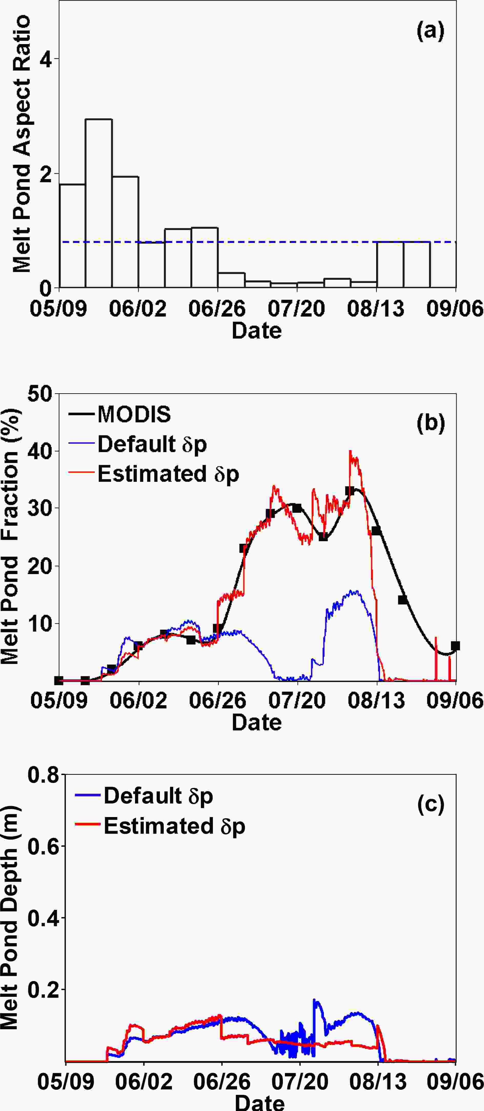 Figure6. (a) The estimated and default aspect ratio for the multi-year ice region. (b) Comparison of MODIS observed melt pond fraction (black solid line; units: %) and the simulation using the estimated (red solid line; units: %) and default aspect ratio (blue solid line; units: %). (c) Comparison of melt pond depth using the estimated (red solid line; units: m) and default aspect ratio (blue solid line; units: m).
The parameter estimation algorithm adjusts the pond aspect ratio parameter continuously to reduce the error of the simulation. In July and August, the simulated MPF using the default parameter is much lower than the observations, and the estimated pond aspect ratio is much smaller than the default value. By using a reduced aspect ratio, the simulated MPF (red line in Fig. 6b) is enhanced and much closer to MODIS observation. This may be explained in the framework of the CESM melt pond scheme. Assuming the meltwater volume remains the same for both the default parameter and the estimated parameter simulation, any reduction of aspect ratio would reduce the depth of the melt pond and enhance the MPF according to Eq. (5). Comparing the simulated melt pond depth with the estimated and default parameter shown in Fig. 6c, it is clear that during the period from 26 June to 13 August when the estimated parameter is reduced, the melt pond depth simulation is enhanced. It is obvious that using the estimated parameter reduces the simulation error of the MPF, whose RMSE is reduced to 7.19%. However, not all the simulations in each period can be improved. For instance, after 13 August, there is no improvement using the estimated parameter. It might indicate that other parameters can have a greater impact on the melt pond evolution at this time. For example, extremely low air temperature would cause the melt pond volume to shrink. In this case, it is not enough to adjust only the pond aspect ratio parameter.
3
3.2.5. Parameter estimation for first-year ice region
For the first-year ice region, the estimated parameter can also improve the MPF simulation. Figure 7a presents the estimated values of the pond aspect ratio parameter on the FYI region. The estimated parameter has a large temporal variation. From 9 May to 18 June, the parameter value is relatively small. From 18 June to 6 September, the estimated parameter value is larger than 10 and remains relatively stable. The large estimated parameter on FYI is probably due to the higher simulated MPF using the default parameter (blue line in Fig. 7b). Compared with MODIS observations, the simulation using the default parameter is quite different and much larger than the observation. After 20 June, while the observed MPF is nearly 0%, the simulated pond fraction using the default value is higher than 15%. The duration of melt ponds is too long given that the MPF is still higher than 20% in early September. The RMSE of the MPF simulation is 6.31%. The simulated MPF using the estimated parameter is decreased and is closer to the MODIS observations. The RMSE is reduced to 4.60%. Using the estimated parameter can reduce the simulation error of MPF. Note that not all the simulation results at each period can be improved. For instance, after June 18, the observed pond fraction drops to zero. The simulated pond fraction fails to capture this observational feature. This indicates that FYI in this region may melt away completely. Although the estimated melt pond parameters are used, this simulation error cannot be eliminated, which shows the limitation of adjusting only one parameter in the melt pond scheme.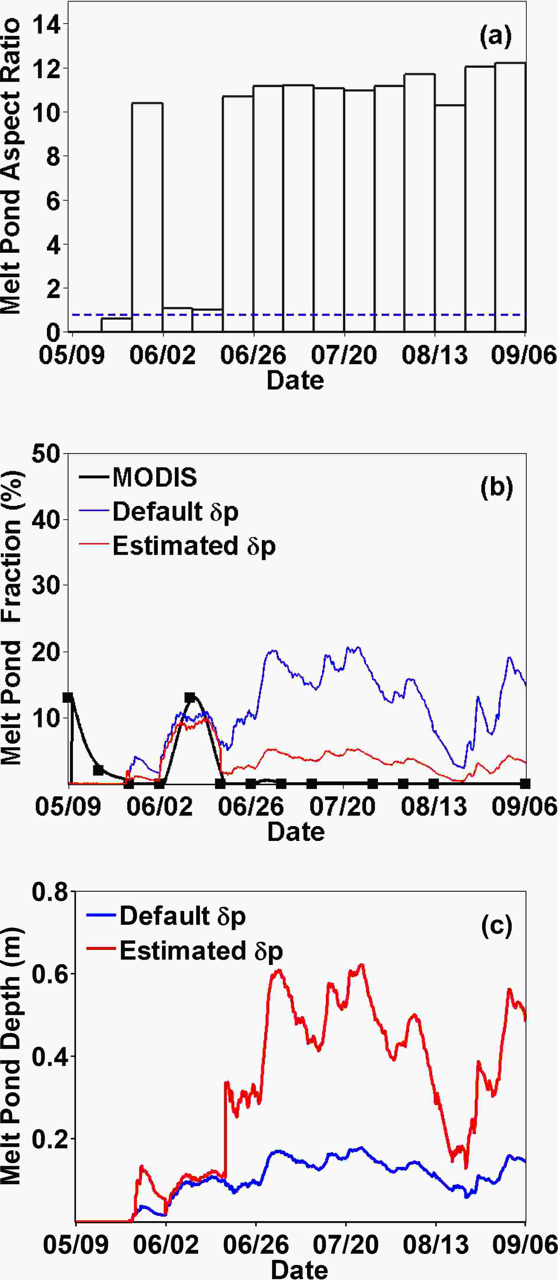 Figure7. (a) The estimated and default aspect ratio for the first-year ice region. (b) Comparison of MODIS observed melt pond fraction (black solid line; units: %) and the simulation using the estimated (red solid line; units: %) and default aspect ratio (blue solid line; units: %). (c) Comparison of melt pond depth using the estimated (red solid line; units: m) and default aspect ratio (blue solid line; units: m).
The adjustment of aspect ratio also causes a change in the melt pond depth simulation consistent with the framework of the CESM melt pond scheme. Figure 7c shows a comparison between the simulated melt pond depth using the estimated parameter and the simulated melt pond depth using the default parameter. Large adjustments of aspect ratio occur from mid-June to the beginning of September. The adjustment of aspect ratio results in reducing the MPF compared to that which is predicted by the simulation which uses the default aspect ratio. By increasing the aspect ratio, the MPF is reduced and much closer to MODIS observation (Fig. 7b). The simulated depth of melt ponds is increased compared with the case using the default aspect ratio since the melt pond volume remains the same for both cases.
3
3.2.6. Discussion of MYI and FYI results
The estimated parameter of FYI is quite different from that of MYI. Previous work has found that the spatio-temporal variable parameters estimated by the adjoint method are more suitable to the simulation of marine ecological models, in contrast to the constant parameters or parameters that only change in space or time (Li et al., 2014). For the melt pond aspect ratio parameter, due to the strong variability of the melt pond process, the spatio-temporal variable parameter may be more reasonable.In general, one would expect that the melt pond aspect ratio for FYI should be lower than that of the MYI, opposite from the result in Fig. 6 and Fig. 7. This may point to the questionable representativeness of the MYI and FYI region selected in our study and the limitation of adjusting only one model parameter. Since only pond aspect ratio is adjusted by the adjoint model, when the simulation using the default parameter is different from the observation, the adjoint model will provide an estimated aspect ratio such that the new simulation is closer to observation. If the other parameter, such as

For both the MYI and FYI region, the parameter estimation algorithm presented in section 2.5 can derive an estimated aspect ratio that can improve the MPF simulation as expected. The adjustment of aspect ratio and the simulation of MPF and depth are consistent in the framework of CESM scheme. However, for both the MYI and FYI regions, there are periods that the adjustment of aspect ratio does not improve the MPF simulation significantly. This may be explained by the fact that the development and temporal evolution of melt ponds are influenced by many factors. Adjusting the aspect ratio has its limitations in improving melt pond simulations.
(1) The direct code transformation method adopted here can correctly obtain the tangent linear model and adjoint model of the melt pond parameterization scheme. The cost function gradient is calculated correctly using the adjoint model. The parameter estimation algorithm composed of the forward model, the adjoint model, and the minimization algorithm is effective in parameter estimation of the CESM melt pond scheme in CICE6.0.
(2) The estimated parameter varies with time and space. This is different from the default fixed parameter in CICE6.0. The estimated parameter values on the MYI and FYI regions during different periods of Arctic summer are quite different. This could be closely related to the strong variability of melt ponds on sea ice.
(3) When used in the simulation, the estimated parameter reduces the simulation error of MPF significantly. In the case study, compared with the experiments using the default parameter, the experiments using the estimated parameter have less RMSE compared with MODIS observations in terms of MPF.
The melt pond behavior involves a complex mechanism that is affected by multiple variables such as radiation, air temperature, precipitation, and sea ice surface topography, etc. In this paper, an adjoint model of the CESM melt pond scheme is developed to estimate the pond aspect ratio parameter. The results prove the feasibility of applying the adjoint model in melt pond parameter estimation. This work provides a foundation for future applications of the adjoint model concerning the estimation of other parameters in melt pond schemes. The melt pond aspect ratio determines the partitioning of meltwater volume between melt pond area and depth. Although this is an important parameter, other parameters cannot be ignored. For instance, the meltwater retaining fraction can directly affect the melt pond volume. Due to complex interactions between physical processes, the adjoint model should be further improved to include more parameters. Multiple parameters should be estimated simultaneously to achieve optimization of the model. Besides, the CESM scheme is relatively simple. Developing an adjoint model for melt pond schemes that have a more complete physical basis and using it to provide parameter estimation would improve the description of melt ponds in sea ice models and ultimately improve their performance. Furthermore, when using an adjoint model to estimate model parameters, the framework of the forward model is accepted as a precondition. This is a limitation of the adjoint model method. More physical consideration should be included to help improve the framework of numeric models and schemes.
Acknowledgments. This research was funded by the National Key R&D Program of China (Grant No. 2018YFA0605904). We thank the CliSAP-Integrated Climate Data Center, University of Hamburg for their online publication of MODIS melt pond data. The comments and suggestions from reviewers and editors helped us greatly in improving the manuscript.
