HTML
--> --> -->The accurate retrieval of land surface characteristic parameters is essential for further estimation of turbulent heat fluxes. Of the land surface characteristic parameters, the land surface broadband albedo and land surface temperature (LST) are vitally important (Han et al., 2016). From the satellite data, the narrowband albedos can be easily obtained, while the conversion from narrowband albedos to broadband albedo remains to be solved for the further calculation of upwelling shortwave radiation flux (SWU). Generally, the broadband albedo can be derived from the narrowband albedos via statistical methods (Zou et al., 2018b). On the one hand, however, the feasibility of this method needs to be further validated against in-situ measurements; whilst on the other hand, such in-situ measurements are also useful for calibration of the empirical coefficients for better applicability over a specific study area. The LST retrieval methods mainly include single-channel algorithms, multi-channel algorithms, and atmospheric correction methods. Of the multi-channel algorithms, the split-window algorithm has been widely used for LST retrieval with numerous successful applications based on AVHRR, MODIS, and FY-2C (Tang et al., 2008; Zhong et al., 2010; Jiang and Liu, 2014; Hu et al., 2018). However, the retrieval methods of surface broadband albedo and LST independently based on the up-to-date FY-4A data have not been established, which may lead to an even wider range of applications.
Land surface turbulent heat fluxes can be monitored via in-situ measurements or remote sensing approaches from polar-orbiting and geostationary satellites. In-situ measurements of meteorological parameters have been used for estimations of land surface heat fluxes. Zou et al. (2018a) applied the combinatory method to estimations of land surface heat fluxes and evapotranspiration using CAMP/Tibet [Coordinated Enhanced Observing Period (CEOP) Asia–Australia Monsoon Project on the Tibetan Plateau] in-situ measurements. Li et al. (2019) used the maximum entropy production model to estimate surface heat fluxes over the central TP based on the observation data of the Third Tibetan Plateau Atmospheric Scientific Experiment. However, in-situ estimations of land surface heat fluxes are limited to the point scale. Thus, data from polar-orbiting and geostationary meteorological satellites are more suitable to derive regional distributions of land surface heat fluxes. In previous studies, compared with geostationary satellites, polar-orbiting satellites have been more widely applied for estimations of land surface turbulent heat fluxes over the TP (Ma et al., 2006, 2009, 2011, 2014; Han et al., 2016; Tang and Li, 2017a, b; Ge et al., 2019). Tang and Li (2017a) first established the constant decoupling factor method for the daily upscaling of evapotranspiration (ET) based on MODIS data. The new method presented definite superiority in accuracy over the widely used constant evaporative fraction method by significantly reducing the underestimation of the daily latent heat flux (LE) via the latter method. Tang and Li (2017b) further developed five methods for converting remotely sensed instantaneous ET to daily values. Results demonstrated that the constant decoupling factor method, the constant surface resistance method, and the constant ratio of surface resistance to aerodynamic resistance method, produced more accurate daily LE estimation than the constant evaporative fraction method and the constant Priestley–Taylor parameter method. Ma et al. (2006) used Landsat-7 ETM data to estimate land surface variables and land surface heat fluxes over the central TP. Ma et al. (2009) applied ASTER imagery to estimate surface fluxes over the northern TP with their absolute percent differences of less than 10%. Ma et al. (2014) used AVHRR and MODIS data for estimation of the surface heating field and LE over the TP, which revealed the estimations of AVHRR were basically consistent with those of MODIS, with the latter generally displaying higher accuracy. Han et al. (2016) applied ASTER data to estimate land surface heat fluxes in the Mt. Everest region over the TP with the topographical effects considered for better applicability to mountainous regions. However, several shortcomings exist in previous studies based on polar-orbiting satellites (Ma et al., 2006, 2009, 2014; Han et al., 2016; Ge et al., 2019). First, the observations via polar-orbiting satellites are mostly between daily to semi-monthly scales, which is relatively much shorter than those based on geostationary satellites and generally leads to data scarcity in ground validation. Second, due to the time discontinuity of polar-orbiting observations, intensive observations of land–atmosphere heat fluxes are still lacking, which are significant for the understanding of the drastic diurnal cycles of physical processes in the atmospheric boundary layer. Third, it is impossible for the overpass time of one polar-orbiting satellite over a specific region to represent the condition of a whole day.
Compared with polar-orbiting satellites, geostationary satellites are more suitable for observation with high temporal continuity. At present, though, applications of geostationary satellites to estimations of land surface turbulent heat fluxes over the TP are much rarer than those of polar-orbiting satellites (Oku et al., 2007; Zhong et al., 2019). Oku et al. (2007) used GMS-5 data to estimate land surface heat fluxes over the TP, while the satellite zenith angle of GMS-5 from the TP is more than 60°, thus the actual field of view over the TP is between 7 and 10 km, and this relatively low spatial resolution over the TP restricts the accuracy in heat flux estimation. Besides, the above study did not cover the entire TP. Zhong et al. (2019) applied FY-2C/SVISSR data to retrieve hourly land surface heat fluxes over the entire TP, while due to the vacancy of shortwave infrared (SWIR) channels of FY-2C/SVISSR, polar-orbiting satellite data were also used for retrieval of land surface characteristic parameters such as Normalized Difference Vegetation Index (NDVI), surface broadband albedo, and surface emissivity, but the input of another satellite data source may introduce some uncertainties into the heat flux estimation. Compared with FY-2C/SVISSR, the up-to-date FY-4A/AGRI covers observations from the visible (VIS) to near-infrared (NIR), the SWIR, the medium-wave infrared (MWIR), and the longwave infrared (LWIR) bands, plus the water vapor bands with channels expanded from 5 to 14 and corresponding spatial resolutions improved from 1.25–5 km to 0.5–4 km. In this study, the FY-4A/AGRI data were used to estimate heat fluxes without the aid of polar-orbiting satellites. Moreover, previous studies on estimations of land surface turbulent heat fluxes over the TP were more focused on their seasonal variations, while a main scarcity lies in the satellite illustrations of their hourly variations with high spatiotemporal continuity.
In order to derive the hourly land surface turbulent heat fluxes over the entire TP independently based on the up-to-date FY-4A/AGRI, a set of algorithms based upon FY-4A/AGRI for retrievals of land surface characteristic parameters and turbulent heat fluxes is presented in this study. The paper is organized as follows. Section 2 introduces the in-situ measurements, satellite data, and meteorological forcing dataset used in this study. Section 3 elaborates on the principles of the algorithms for retrievals of land surface characteristic parameters and turbulent heat fluxes based on FY-4A. The results are displayed and discussed in section 4, the main conclusions are drawn in section 5, and the detailed retrieval methods for surface broadband albedo and LST are explained in the Appendix.
2.1. Tibetan Observation and Research Platform in-situ data
The Tibetan Observation and Research Platform (TORP) is a project aimed at research on the land surface process over the TP, which comprises various comprehensive observation and research stations and other additional observational sites (Ma et al., 2008). The locations of the comprehensive observation and research stations used in this study are marked in Fig. 1, and their detailed information is listed in Table 1. The TORP in-situ measurements, with a temporal resolution of 30 minutes, were used to develop the retrieval algorithms and carry out the cross validation.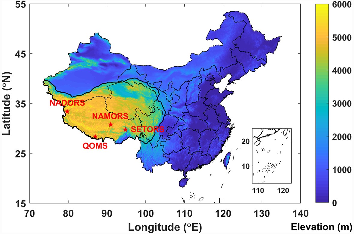 Figure1. Locations of the Tibetan Plateau (black thick line) and in-situ meteorological stations (red stars) from TORP.
| Station | Longitude (°E) | Latitude (°N) | Altitude (m) | Heat fluxes measurements for ground validation |
| NADORS | 79.7035 | 33.39056 | 4270 | SWD, SWU, LWD, LWU, Rn |
| NAMORS | 90.9636 | 30.7699 | 4730 | H, LE |
| QOMS | 86.949638 | 28.358209 | 4276 | SWD, SWU, LWD, LWU, Rn, H |
| SETORS | 94.7417 | 29.7622 | 3326 | SWD, SWU, LWD |
| Notes: SWD, downwelling shortwave radiation flux; SWU, upwelling shortwave radiation flux; LWD, downwelling longwave radiation flux; LWU, upwelling longwave radiation flux; Rn, net radiation flux; H, sensible heat flux; LE, latent heat flux. | ||||
Table1. Information on the TORP stations for ground validation.
2
2.2. FY-4A geostationary satellite data
The Fengyun-4 geostationary satellite system, the successor of Fengyun-2, is the second generation of the Chinese geostationary meteorological satellite system. Launched on 11 December 2016, Fengyun-4A (FY-4A) is the first test satellite of the Fengyun-4 system. The Level 1 data of FY-4A started on 12 March 2018. FY-4A provides two modes of data telemetering: the China region mode, and the full disk mode, which covers the Asia and Oceania region. The temporal resolution of FY-4A Level 1 data can reach 15 minutes (Min et al., 2017). The meteorological instruments onboard FY-4A include the Advanced Geostationary Radiation Imager (AGRI), the Geostationary Interferometric Infrared Sounder (GIIRS), the Lightning Mapping Imager (LMI), and the Space Environment Monitoring Instrument Package (SEP) (Yang et al., 2017). The band list of FY-4A/AGRI is displayed in Table 2. Compared with FY-2/VISSR, the imaging observation bands of multichannel scan imagery radiometer FY-4A/AGRI have been expanded from 5 channels to 14 channels. Of the total 14 spectral bands of FY-4A/AGRI, channels 1–3 cover the VIS to NIR bands, channels 4–6 cover the SWIR bands, channels 7–8 cover the MWIR bands, channels 9–10 are the water vapor bands, and channels 11–14 cover the LWIR bands. The spatial resolutions of the VIS to NIR, SWIR, MWIR and LWIR bands are 0.5–1 km, 2 km, 2–4 km and 4 km, respectively. In this study, channels 2–3 were used to calculate the NDVI, channels 1–6 were used for broadband albedo retrieval, and channels 12–13 were applied for estimation of LST (Fig. 2). For the spatial resolution differences of FY-4A/AGRI bands, in order to reduce the errors due to resolution mismatch, the finer spatial resolution bands should be upscaled to the same resolution as those bands with coarser resolution, i.e., from 0.5–2 km to 4 km resolution. Fortunately, for each band of FY-4A/AGRI, data with coarser resolution of 4 km were already provided on the official website. Therefore, the 4 km resolution data for all bands were uniformly used for subsequent surface characteristic parameter retrieval and turbulent heat flux estimation in this study.| Band | Wavelength range (μm) | Central wavelength (μm) | Spatial resolution (km) |
| 1 | 0.45–0.49 | 0.47 | 1 |
| 2 | 0.55–0.75 | 0.65 | 0.5 |
| 3 | 0.75–0.90 | 0.83 | 1 |
| 4 | 1.36–1.39 | 1.37 | 2 |
| 5 | 1.58–1.64 | 1.61 | 2 |
| 6 | 2.10–2.35 | 2.22 | 2 |
| 7 | 3.50–4.00 | 3.72 | 2 |
| 8 | 3.50–4.00 | 3.72 | 4 |
| 9 | 5.80–6.70 | 6.25 | 4 |
| 10 | 6.90–7.30 | 7.10 | 4 |
| 11 | 8.00–9.00 | 8.50 | 4 |
| 12 | 10.3–11.3 | 10.8 | 4 |
| 13 | 11.5–12.5 | 12.0 | 4 |
| 14 | 13.2–13.8 | 13.5 | 4 |
Table2. Band list of FY-4A/AGRI.
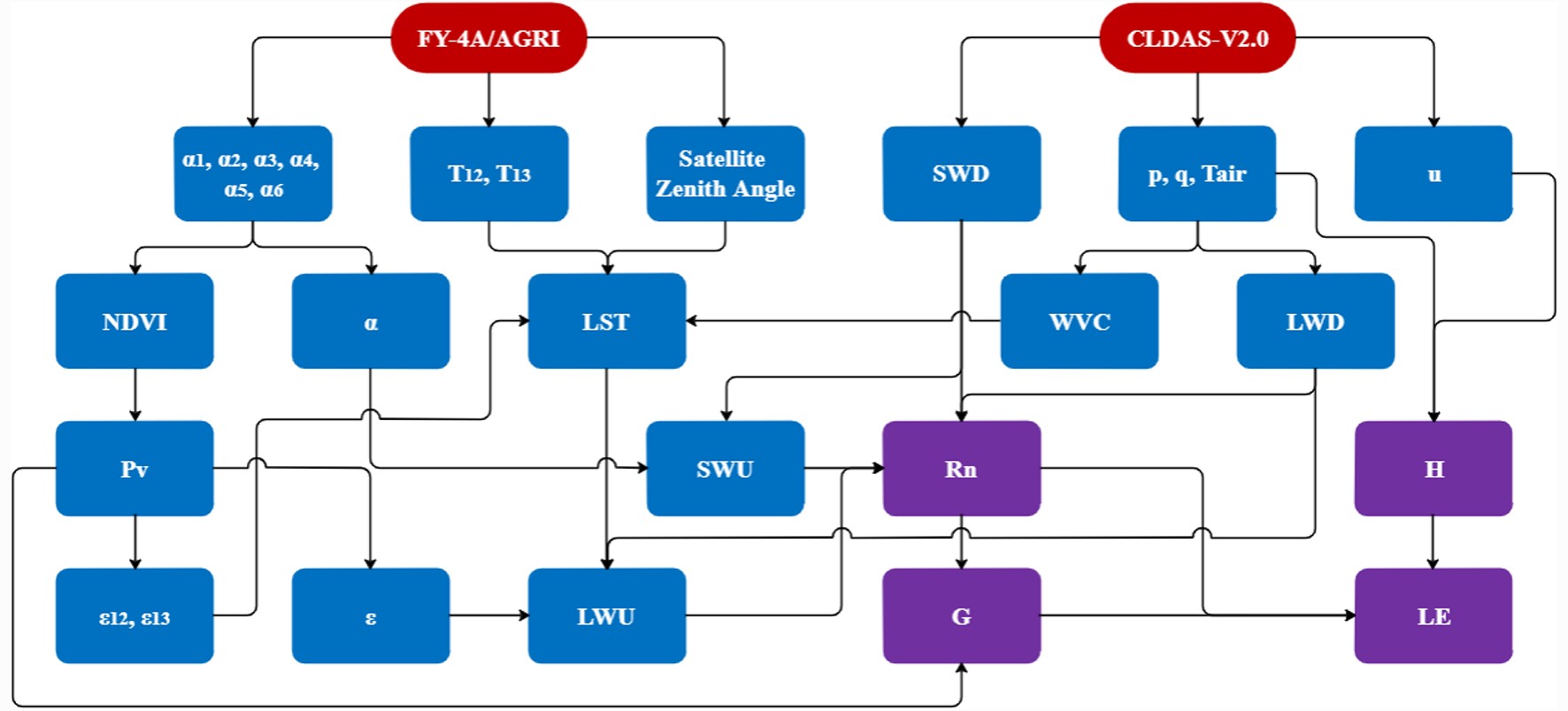 Figure2. Flowchart of the retrieval method of the land surface characteristic parameters and heat fluxes by combining FY-4A/AGRI and CLDAS-V2.0 data (α1–α6, narrowband albedos of FY-4A/AGRI spectral bands 01–06; T12 and T13, brightness temperatures monitored in band 12 and 13 of FY-4A/AGRI, respectively; SWD, downwelling shortwave radiation flux; p, near-surface air pressure; q, specific humidity at 2 m, Tair, air temperature at 2 m; u, wind speed at 10 m; NDVI, Normalized Difference Vegetation Index; α, surface broadband albedo; LST, land surface temperature; WVC, atmospheric water vapor content; LWD, downwelling longwave radiation flux; Pv, proportion of vegetation; SWU, upwelling shortwave radiation flux; Rn, net radiation flux; H, sensible heat flux; ε12 and ε13, narrowband emissivities of band 12 and 13 of FY-4A/AGRI, respectively; ε, land surface broadband emissivity; LWU, upwelling longwave radiation flux; G, soil heat flux; LE, latent heat flux).
For the clear detection on FY-4A/AGRI, the threshold method (Oku et al., 2007) was used in this study. For bands 12–13, brightness temperature values below 250 K were not used in the LST retrieval. The threshold of 250 K was determined based on TORP in-situ measurements to acclimate the general climatic condition over the TP in spring. Due to the presence of cloud, the cloud-top temperature instead of the surface temperature will be detected, which yields an underestimation in brightness temperature and thus a lower LST. The underestimation in LST will further induce underestimation in LWU (upwelling longwave radiation flux) and H (sensible heat flux). Additionally, areas covered by clouds will also exhibit higher surface broadband albedo than those under clear-sky conditions. The overestimation in surface broadband albedo will result in overestimation in SWU. Therefore, the abnormal low brightness temperature data points were considered as cloudy and then eliminated based on this threshold. However, several defects also exist in the threshold method. First, the selection of the threshold is difficult to determine, for this one-size-fits-all approach may induce some uncertain missing reports and false alarms. Second, due to the land cover heterogeneity over the TP, the threshold method is not sufficient to meet the unique hydrometeorological conditions over the whole TP. It should be noted that the FY-4A Level-2 CLM (cloud mask) product is also available for clear detection. However, the areal proportion of the clear region over the whole TP detected via the FY-4A CLM product is too small (< 20%) for most observation times, from which it is difficult to derive the spatial distributions of the surface characteristic parameters. Thus, the threshold method was used for the clear detection in this study.
2
2.3. China Land Data Assimilation System meteorological forcing dataset
For estimation of the radiation flux components and turbulent heat fluxes, meteorological forcing data are needed as inputs. In this study, the CLDAS (China Land Data Assimilation System) meteorological forcing dataset, CLDAS-V2.0, was used in combination with FY-4A satellite data for flux estimation. CLDAS-V2.0 has a spatial resolution of 0.0625° × 0.0625° and a temporal resolution of 1 h, and covers the whole East Asia region (0°–65°N, 60°–160°E) from 19 January 2017. The near-surface air pressure p, specific humidity q measured at 2 m, air temperature Tair measured at 2 m, horizontal wind speed u measured at 10 m, and surface downwelling shortwave radiation flux (SWD) were used as the input data. For integration of the CLDAS-V2.0 with FY-4A satellite data, the FY-4A data were upscaled from the original 4 km × 4 km normalized projection grid to the 0.0625° × 0.0625° equal latitude and longitude grid of CLDAS-V2.0 using bilinear spatial interpolation.3.1. Retrieval of land surface broadband albedo
Since the TORP in-situ measurements already covered the observation for the radiation flux components, the in-situ albedo αobs was directly calculated aswhere SWDobs and SWUobs are the ground observed downwelling shortwave radiation flux and upwelling shortwave radiation flux, respectively.
Of the total 14 spectral bands of FY-4A, the VIS to SWIR bands 1–6 are suitable for broadband albedo retrieval. Based on the linear regression method discussed in the Appendix, a linear relationship between αobs and the narrowband albedos of these six spectral bands α1–α6 can be established to work out the linear fitting coefficients k0–k6:
where e is the error between the observed broadband albedo αobs and the fitted value of the broadband albedo α, and α was computed through the derived k0–k6:
Note that the time series of αobs were divided into two halves: the first half for solving the linear fitting coefficients k0–k6 [Eq. (2) and Eq. (A13)] and then the calculation of α [Eq. (3)], and the second half for the validation of α against αobs. The validation result is discussed in section 4.1.
2
3.2. Retrieval of LST
The in-situ land surface temperature, LSTobs, was directly computed as (Chen et al., 2017; Hu et al., 2018)where LWDobs and LWUobs are the ground observed downwelling longwave radiation flux and upwelling longwave radiation flux, respectively, σ is the Stefan–Boltzmann constant (5.67 × 10?8 W m?2 K?4), and ε is the land surface broadband emissivity. The latter was calculated via (Valor and Caselles, 1996; Ma et al., 2003)
where εv = 0.985 and εs = 0.960 are the land surface emissivity for full vegetation and bare soil, respectively (Valor and Caselles, 1996), <dε> = 0.015 represents the cavity effect of rough surfaces, and Pv is the proportion of vegetation, which was derived as (Zou et al., 2018b)
where the NDVI was obtained from (Carlson and Ripley, 1997)
in which α2 and α3 are the narrowband albedos of band 2 and band 3 of FY-4A/AGRI (Table 2), respectively, and the NDVImin and NDVImax in Eq. (6) are NDVI values for bare soil and full vegetation, respectively. In this study, we set NDVImin = 0 and NDVImax = 0.8.
In order to retrieve the LST from satellite remote sensing, the Split-Window Algorithm (SWA) of Becker and Li (1995) was used in this study:
where LST is the satellite-retrieved land surface temperature (K); T12 and T13 are the brightness temperatures (K) monitored in band 12 and band 13 of FY-4A/AGRI (Table 2), respectively; w is the water vapor content (WVC, g cm?2), which was calculated via Eq. (10) (Yang et al., 2006); θ is the satellite zenith angle;

where Tair is the air temperature (K) and RH is the relative humidity (%) calculated via
in which ea (Pa) and es (Pa) are the actual and saturated water vapor pressure, respectively:
where p is the air pressure (Pa) and q is the specific humidity (kg kg?1) (Zou et al., 2018a).
Similar to the albedo retrieval process, the derivation of k0–k12 for LST was also based on Eq. (A13). The validation of LST against LSTobs is also discussed in section 4.1.
2
3.3. Estimation of radiation flux components
After the broadband albedo α was retrieved, the upwelling shortwave radiation flux SWU can be obtained from α and the downwelling shortwave radiation flux SWD provided by the CLDAS meteorological forcing data:The downwelling longwave radiation flux LWD can be calculated from the air temperature Tair (K) and the actual water vapor pressure ea (Pa) (Brutsaert, 1975):
where λ was set as 1.31.
Then, the upwelling longwave radiation flux LWU was derived from the LST, LWD, and the land surface broadband emissivity ε (Han et al., 2016):
2
3.4. Estimation of turbulent heat fluxes
The net radiation flux Rn was obtained from the radiation flux components:The soil heat flux G was calculated from Rn and Pv:
where rv = 0.05 and rs = 0.315 are the ratios of soil heat flux to net radiation flux for full vegetation and bare soil, respectively.
In this study, the SEBS (Surface Energy Balance System) model (Su, 2002) was used for estimation of the hourly sensible and latent heat flux. The SEBS model has been successfully applied for the estimation of daily, monthly and annual evaporation at both local and regional scales under all atmospheric stability regimes (Tang et al., 2011). Characteristically, SEBS is effective for estimating land surface heat fluxes in semiarid areas (Su et al., 2003a) and for drought monitoring (Su et al., 2003b). Besides, SEBS was also firstly coupled with a numerical weather prediction model by Jia et al. (2003) and firstly used in data assimilation by Wood et al. (2003).
The derivation of sensible heat flux H requires the solution of a set of three equations:
where L is the Obukhov length, ρ is the air density, cp is the specific heat capacity at constant pressure, θv is the virtual potential temperature, u* is the friction velocity, k = 0.4 is von Karman’s constant, g is the gravitational acceleration, u is the horizontal wind speed, z is the reference height, d0 is the zero plane displacement height, z(0,m) and z(0,h) are the roughness heights for momentum and heat transfer, respectively, Ψm and Ψh are the stability correction functions for momentum flux and heat flux, respectively, and θ0 and θa are the surface potential temperature and the air potential temperature, respectively. L, u* and H are the three unknown variables in Eqs. (21)–(23). Due to the implicit functional relationship of L, u* and H, these three unknown variables were solved via iteration (Ge et al., 2019). After H was worked out, the LE can be directly calculated as the remainder term of the surface energy balance equation (Su, 2002).
2
3.5. Statistical indices for ground validation
In order to examine the accuracy in land surface characteristic parameter retrieval and turbulent heat flux estimation, four statistical indices, RMSE (root-mean-square error), MB (mean bias), MAE (mean absolute error), and R (Pearson correlation coefficient) were used:4.1. Validation of broadband albedo and LST
Scatterplots of the FY-4A retrieved broadband albedo and LST against TORP in-situ measurements are shown in Figs. 3a and b. The RMSE, MB, MAE and R of broadband albedo retrieval were 0.0309, ?0.0003, 0.0229 and 0.683, respectively. From Fig. 3a, we can find clusters of points indicating different ground validation stations. Of these three stations, at NADORS the FY-4A estimates were in best accordance with the TORP measurements, which may result from the much more homogeneous underlying surface of NADORS. The broadband albedo at SETORS, which is located in a highly vegetated region, was the smallest relatively, and the satellite estimates showed a slight overestimation. Meanwhile, at the sparsely vegetated QOMS, the situation was just the opposite. The systematic underestimation of broadband albedo at QOMS may result in the slightly negative MB, while overall the broadband albedo retrieval showed a relatively small RMSE. The RMSE, MB, MAE and R of LST retrieval were 3.85 K, 0.19 K, 3.24 K and 0.962, respectively. The MB showed a slight overestimation of LST, which may possibly be due to the overestimation in low values at NADORS. We also validated the MOD11C1 daily LST product against the TORP measurements in April 2018 over the TP, which is shown in Fig. 3c. The results show that the RMSE of LST was 6.56 K, and the MB was ?0.20 K. The accuracy of LST retrieved from FY-4A/AGRI was superior than that from MOD11C1, which also verified that the universal algorithm may not work well for the TP. Generally, the small RMSEs of broadband albedo and LST retrieval verified the applicability of the regression scheme based on FY-4A/AGRI over the TP. Thus, the retrieved broadband albedo and LST were further used to calculate the SWU and LWU, respectively, whose estimation accuracy may largely depend on the retrieval of broadband albedo and LST.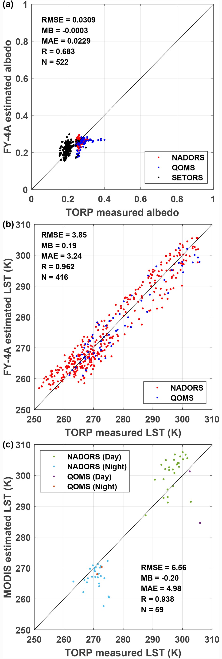 Figure3. Validation of the (a) land surface broadband albedo and (b) LST retrieved by FY-4A/AGRI and (c) LST retrieved by MOD11C1 against the TORP in-situ measurements.
2
4.2. Validation of radiation flux components and turbulent heat fluxes
Scatterplots of the estimated SWD, SWU, LWD and LWU against TORP in-situ measurements are displayed in Figs. 4a–d. It is noted that the estimated SWD was directly obtained from the CLDAS-V2.0 product, and the LWD was also directly calculated from the air temperature, air pressure and specific humidity of CLDAS-V2.0 [Eq. (17) and Eq. (12)]. The RMSE and MB of SWD were 138.87 W m?2 and 45.69 W m?2, and those of LWD were 51.55 W m?2 and ?41.17 W m?2, indicating that the CLDAS-V2.0 product may have an overestimation for SWD and an underestimation for LWD. The MB of SWD may mainly result from the overestimation in low values at SETORS, and the large MB of LWD may be due to the underestimation of air temperature in CLDAS-V2.0. From Fig. 4, it can be seen that the biases in SWD, SWU and LWD were all largest at SETORS station, which may result from its geolocation situation with heterogeneous land cover. SETORS station lies in a valley basin surrounded by mountains. The nearest CLDAS-V2.0 grid point to SETORS station has a higher elevation than the station. Therefore, the CLDAS-V2.0 air temperature at the grid scale was relatively lower than the point measurements, contributing to an underestimation in LWD [Eq. (17)]. Additionally, SETORS is humid and cloudy all year round. We speculate that, due to the presence of clouds, the in-situ SWD is weakened while the in-situ LWD is strengthened compared with CLDAS-V2.0 data. The SWD and LWD were both directly obtained as discussed above, while the SWU and LWU were both derived with the FY-4A data involved. The RMSE and MB of SWU were 32.78 W m?2 and 9.43 W m?2, and those of LWU were 17.92 W m?2 and ?0.15 W m?2, revealing a slight overestimation of SWU and a nearly unbiased estimation of LWU. Compared with SWD and LWD, the relatively smaller RMSEs and MBs of SWU and LWU verified the accuracy of broadband albedo and LST retrieval from another point of view.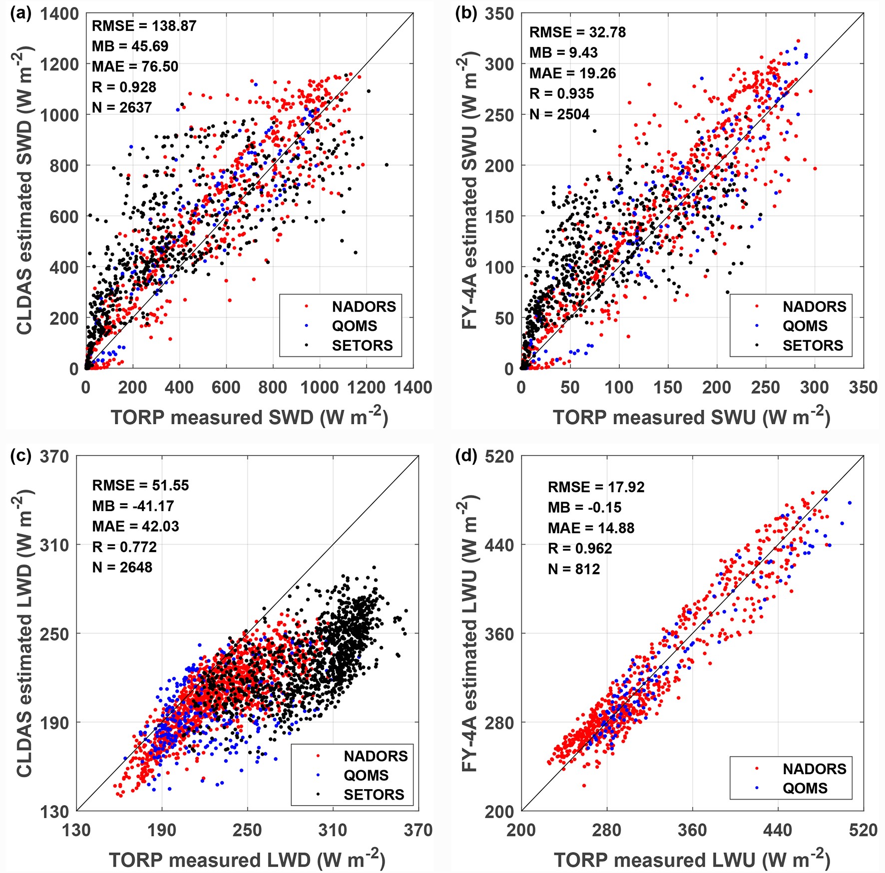 Figure4. Validation of the (a) downwelling shortwave radiation flux, (b) upwelling shortwave radiation flux, (c) downwelling longwave radiation flux and (d) upwelling longwave radiation flux against the TORP in-situ measurements.
Scatterplots of FY-4A estimated Rn, H and LE against TORP in-situ measurements are shown in Figs. 5a–c. The RMSE and MB of Rn were 58.88 W m?2 and 12.24 W m?2. From Fig. 5a we can see a precise estimate of nighttime Rn, while the daytime Rn at both sites, especially at QOMS, was generally overestimated, which may result in the positive MB. Additionally, on the MB of Rn, the overestimation of SWD and underestimation of LWD discussed above may have offset each other. The RMSE and MB of H were 82.56 W m?2 and ?31.65 W m?2, and those of LE were 72.46 W m?2 and 31.60 W m?2, depicting an underestimation of H and an overestimation of LE. From Fig. 5b, the negative MB of H was mainly due to the systematic underestimation during nighttime. According to the surface energy balance equation (Kustas and Norman, 1997; Su, 2002), the underestimation of H results in the overestimation of LE, which may explain the abnormal high points during nighttime in Fig. 5c and the positive MB of LE. Chen et al. (2019) also pointed out that the underestimation of H and the overestimation of LE may result from the overestimation of kB?1 in the SEBS model. Additionally, the diurnal cycles of kB?1 may also contribute to the nighttime underestimation and daytime overestimation of H, which will be focused upon in our future studies for some possible model improvements. Moreover, the spatial resolutions of CLDAS-V2.0 and FY-4A data are 0.0625° (~7 km) and 4 km, respectively (the FY-4A retrieved 4 km LST was upscaled to a 0.0625° grid to match the air temperature data of CLDAS-V2.0), while the “ground truths” of TORP in-situ measurements can only represent a spatial scale of approximately 10–100 m. The scale difference of air temperature between TORP measurements and CLDAS-V2.0 reanalysis data, and the scale difference of LST between TORP measurements and FY-4A satellite data, may both contribute to the day/night discrepancies of H estimation. We are going to use the polar-orbiting satellite data with higher spatial resolution as a bridge to reduce the scale differences for better estimation of H in our future studies. Moreover, due to the surface energy balance closure problem (Foken, 2008; Zhong et al., 2009; Leuning et al., 2012), the sum of G, H and LE is generally less than Rn, and thus when the LE is derived as the remainder term of the surface energy balance equation, this derived LE is usually higher than its actual value.
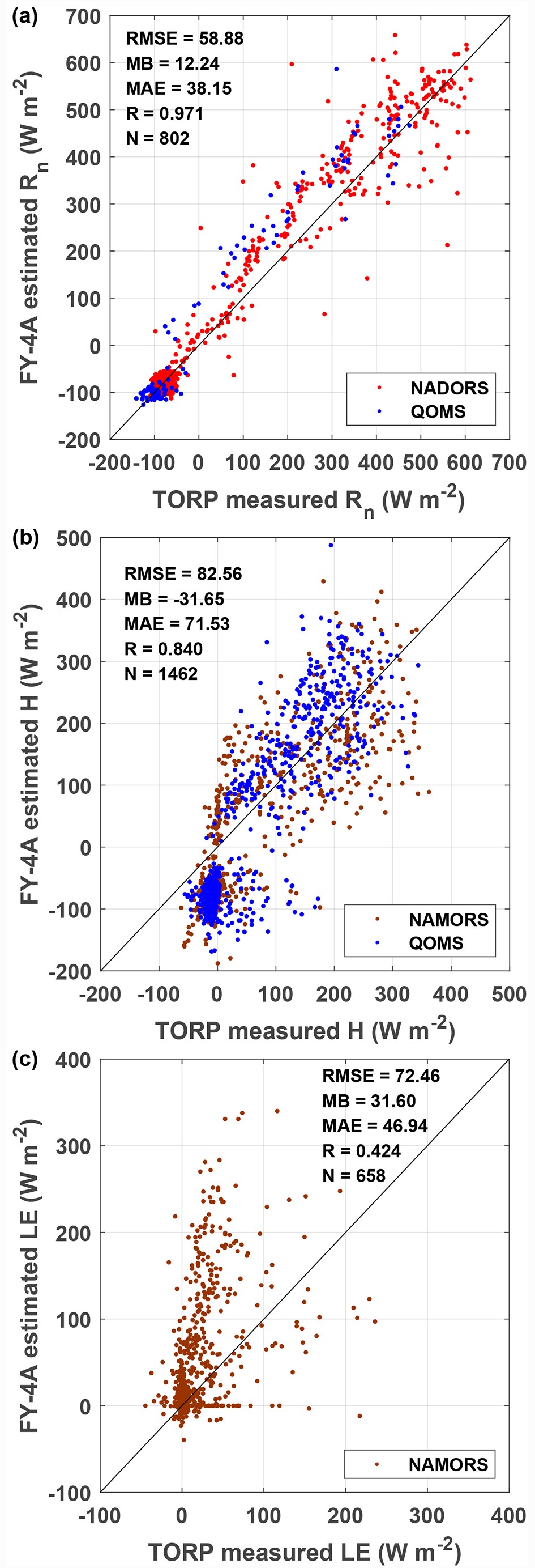 Figure5. Validation of the (a) net radiation flux, (b) sensible heat flux and (c) latent heat flux estimated by FY-4A/AGRI against the TORP in-situ measurements.
2
4.3. Spatial distributions for diurnal variations of LST and turbulent heat fluxes
The spatial distribution of the diurnal variation of LST in April 2018 is shown in Fig. 6. Since the nighttime LST changes slowly, Fig. 6 only displays the diurnal variation in the daytime, i.e. 0800–1900 (Local Standard Time). We can see that the LST over the TP varied from 250 K to 310 K, generally reaching a maximum at 1300. The southeastern TP was the high-value zone of LST throughout the day, which may result from the effect of excessive atmospheric WVC compared with the whole TP in the split-window algorithm for LST retrieval. Additionally, the LST over the Qaidam basin depicted distinctive characteristics, which basically maintained as a high-value zone compared with the surrounding regions, especially at noon. This phenomenon may result from its low-lying terrain and desert environment. Generally, the LST over the TP presented a rapid hourly variability, which was especially distinct in the heating processes over the Qaidam basin as well as the mountainous regions of the southwestern TP from 1100 to 1300 and the cooling processes over the central TP from 1400 to 1700. The hourly variations of LST over these regions can exceed 10 K, which revealed the unique thermodynamic property of the TP.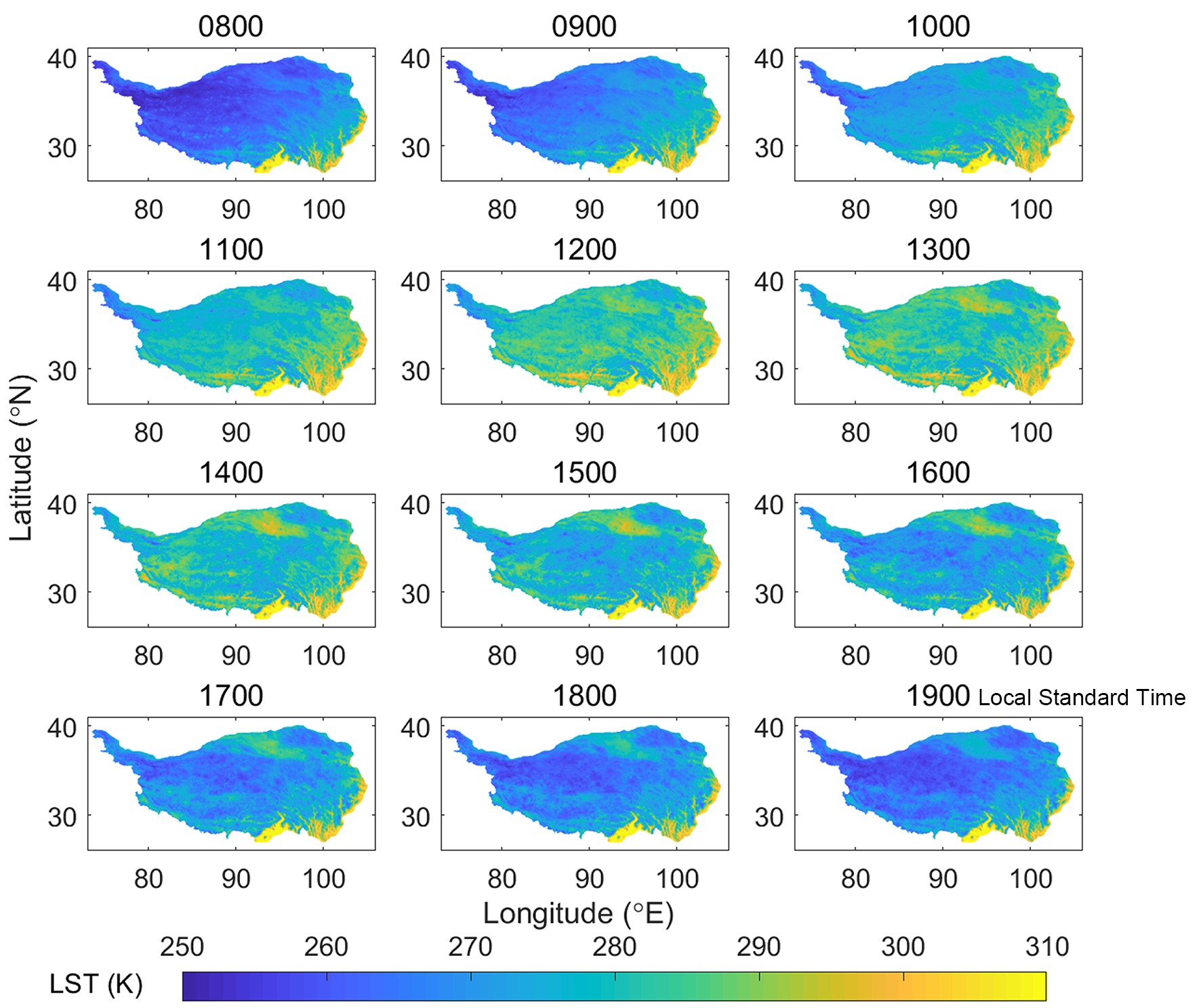 Figure6. Diurnal variation of the LST over the TP in April 2018 retrieved from FY-4A/AGRI.
The spatial distributions of the diurnal variations of Rn, H and LE in April 2018 are shown in Figs. 7–9, which also only exhibit the daytime diurnal variations due to the slight changes of turbulent heat fluxes at night. The Rn varied from ?200 W m?2 to 800 W m?2, displaying a distinct high-value zone in the central TP. Besides, the low-value zone in the southeastern TP was likely due to the higher LST in this region, which can further derive a higher LWU. The ranges of H and LE were from ?200 W m?2 to 500 W m?2 and ?100 W m?2 to 400 W m?2, respectively, overall with H larger than LE over the whole TP in April. Similar to Rn, the high-value zones of H were mainly situated in the central TP, while LE presented a relatively slighter diurnal variation, which for the majority of the TP region varied from 0 to 300 W m?2. Additionally, the low-value zone in the southeastern TP may be influenced by two factors: the Rn and the atmospheric WVC. In the southeastern TP, the lower Rn may outstrip the excessive atmospheric WVC, which ultimately resulted in a relatively low LE. Overall, both the Rn and H exhibited swift hourly variations, especially in their enhancements over the central and northeastern TP from 1100 to 1400. Compared with Rn and H, a relatively subtler hourly variation of LE can also be discerned over the central and eastern TP from 1000 to 1200.
 Figure7. Diurnal variation of the land surface Rn over the TP in April 2018 estimated from FY-4A/AGRI.
In previous studies, surface turbulent heat fluxes were mainly estimated using polar-orbiting satellites including MODIS and AVHRR with coarse spatial resolution, as well as ASTER and Landsat with fine spatial resolution. Contrary to studies based on MODIS and AVHRR (Ma et al., 2011, 2014), FY-4A/AGRI provides far more scenes for ground validation. Compared with studies based on ASTER and Landsat, FY-4A/AGRI supplies hourly-scale turbulent heat flux estimation over the entire TP (Ma et al., 2006; Han et al., 2016; Ge et al., 2019). Studies based on geostationary satellites are much fewer. Oku et al. (2007) applied Geostationary Meteorological Satellite (GMS)-5 data for surface heat flux estimation, while the western TP was not covered via GMS-5. Zhong et al. (2019) first applied the FY-2C/SVISSR data to estimate the hourly surface turbulent heat fluxes over the entire TP. The annual mean spatial distributions of H and LE showed that the central and western TP were the high-value zones of H, while those of LE were mainly located in the southern and eastern TP. From Figs. 8–9, it can also be seen that the spatial distributions of H and LE have a contrary and complementary pattern. Compared with the findings of Zhong et al. (2019), the results in this study can draw a similar conclusion. Overall, the accuracy of surface heat flux estimation in this study is superior to that of Oku et al. (2007), and is at a comparable level with Zhong et al. (2019). Owing to the high temporal resolutions of FY-4A/AGRI and CLDAS-V2.0 data, the delicate hourly variabilities of LST and land surface turbulent heat fluxes can be clearly identified.
 Figure8. Diurnal variation of the land surface H over the TP in April 2018 estimated from FY-4A/AGRI.
 Figure9. Diurnal variation of the land surface LE over the TP in April 2018 estimated from FY-4A/AGRI.
(1) Statistical methods were applied for calibration of the fitting coefficients in broadband albedo and LST retrieval for a better applicability over the TP. The RMSE, MB, MAE and R of broadband albedo retrieval were 0.0309, ?0.0003, 0.0229 and 0.683, respectively, and those of LST retrieval were 3.85 K, 0.19 K, 3.24 K and 0.962, respectively. The relatively small RMSEs and MBs enabled the further estimations of surface heat fluxes over the TP.
(2) The hourly data of surface heat fluxes over the TP were firstly obtained based on FY-4A. The estimated radiation flux components and turbulent heat fluxes were also validated against the in-situ measurements. The RMSEs of SWD, SWU, LWD, LWU, Rn, H, and LE were 138.87 W m?2, 32.78 W m?2, 51.55 W m?2, 17.92 W m?2, 58.88 W m?2, 82.56 W m?2 and 72.46 W m?2, respectively, and those of MBs were 45.69 W m?2, 9.43 W m?2, ?41.17 W m?2, ?0.15 W m?2, 12.24 W m?2, ?31.65 W m?2 and 31.60 W m?2, respectively.
(3) The LST, Rn, H and LE all showed distinct diurnal variations in daytime. In April over the TP, LST varied from 250 K to 310 K, Rn varied from ?200 W m?2 to 800 W m?2, H varied from ?200 W m?2 to 500 W m?2, and LE varied from ?100 W m?2 to 400 W m?2. The hourly variabilities of LST, Rn, H and LE were in good agreement with the intense diurnal cycle of the atmospheric boundary layer over the TP.
Retrieving the land surface characteristic parameters and turbulent heat fluxes via satellite remote sensing is not an easy task. The original observational errors of the in-situ measurements, the interpolations between different projection pixels of satellite data and reanalysis products, and different parameterization schemes for land surface characteristic parameters and turbulent heat fluxes, may all contribute to the errors between satellite estimations and in-situ “true values”. In future studies, multi-source geostationary satellite data, such as Himawari-8/AHI combined with FY-4A/AGRI, will be used for cross-sensor validation of the land surface characteristic parameters, which may serve as an effective supplement to the in-situ validation. Additionally, the latest coordinated observation data from the Second Tibetan Plateau Scientific Expedition will also be used for improvements of the land surface heat flux parameterization schemes.
Acknowledgements. This research was jointly funded by the Second Tibetan Plateau Scientific Expedition and Research Program (Grant No. 2019QZKK010305), the Strategic Priority Research Program of the Chinese Academy of Sciences (Grant No. XDA20060101), the National Natural Science Foundation of China (Grant Nos. 41875031, 91837208, 41522501 and 41275028), the Chinese Academy of Sciences Basic Frontier Science Research Program from 0 to 1 Original Innovation Project (Grant No. ZDBS-LY-DQC005-01), and the Chinese Academy of Sciences (Grant No. QYZDJ-SSW-DQC019). The FY-4A data can be obtained from
The linear relation between the predictand and the factors can be written as
where yi is the ith sample of a specific predictand, which depends upon p factors; xij is the ith sample for the jth factor; k0–kp are the p + 1 linear fitting coefficients; and ei is the ith error between the predictand and the fitted value. The yi, xij, kj and ei can all be rewritten in matrix form:
Thus, Eq. (A1) can be simplified as
Each fitted value is denoted as
which can also be simplified as
In order to derive the fitting coefficients k0–kp, the sum-of-squared differences of the total samples of the predictand and the fitted value, Q, is calculated:
The optimal fitting demands that Q reaches its minimum, which certainly satisfies
Equation (A10) can be rewritten in matrix form:
Thus, the matrix of the linear fitting coefficients k0–kp, K, is finally worked out:
Consequently, the linear fitting equation is obtained after the derivation of k0–kp [Eq. (A7) or Eq. (A8)].
For the retrieval of both α and LST in this study, Y originates from the TORP in-situ measurements, while X stems from the FY-4A satellite data combined with the CLDAS meteorological forcing data. The former represents the ground observation, while the latter signifies the satellite remote sensing. Thus, K is determined and influenced from both these aspects. Next, this linear regression method was applied to the retrieval of α and LST, which is explained in section 3.1 and section 3.2, respectively.
