HTML
--> --> -->| Database profile | |
| Database title | CAS-LSM datasets for the CMIP6 Land Surface Snow and Soil Moisture Model Intercomparison Project |
| Time range | land-hist-gswp3: 1901?2014; land-hist-princeton: 1901?2012; land-hist-crujra: 1901?2014; land-hist-wfdei: 1901?2014 |
| Geographical scope | Global |
| Data format | The Network Common Data Form (NetCDF) version 4 |
| Data volume | land-hist-gswp3: 99.1 GB; land-hist-princeton: 95.6 GB; land-hist-crujra: 97.9 GB; land-hist-wfdei: 97.8 GB |
| Data service system | https://doi.org/10.22033/ESGF/CMIP6.2052 |
| Sources of funding | Second Tibetan Plateau Scientific Expedition and Research Program (STEP) (Grant No. 2019QZKK0206); Youth Innovation Promotion Association CAS; National Natural Science Foundation of China (Grant No. 41830967); National Key Scientific and Technological Infrastructure project "Earth System Science Numerical Simulator Facility" (EarthLab) |
| Database composition | The shared database contains 64 types of data: four experiments multiplied by 16 variables: 1. land-hist-gswp3 dataset comprises 16 files containing 16 variables between 1901 and 2014; 2. land-hist-princeton dataset comprises 16 files containing 16 variables between 1901 and 2012; 3. land-hist-crujra dataset comprises 16 files containing 16 variables between 1901 and 2014; 4. land-hist-wfdei dataset comprises 16 files containing 16 variables between 1901 and 2014 |
The Land Surface Model for the Chinese Academy of Sciences (CAS-LSM) was developed at the Institute of Atmospheric Physics (IAP), CAS (Xie et al., 2018a; Wang et al., 2019; Wang et al., 2020b). It is the land component of the climate system models of CMIP6: the CAS Flexible Global-Ocean-Atmosphere-Land System Model Grid-point version 3 (CAS FGOALS-g3), which was developed at the State Key Laboratory of Numerical Modeling for Atmospheric Sciences and Geophysical Fluid Dynamics (LASG) of the Institute of Atmospheric Physics (IAP), CAS (Li et al., 2020). Based on the experiment design for CMIP6 (Eyring et al., 2016), many CMIP6 experiments based on CAS FGOALS-g3 have been conducted, including the Diagnostic, Evaluation, and Characterization of Klima (Li et al., 2020), historical simulations, Scenario Model Intercomparison Project (Pu et al., 2020), Flux-Anomaly-Forced Model Intercomparison Project (Wang et al., 2020a), Ocean Model Intercomparison Project (OMIP; Lin et al., 2020), Paleoclimate Modeling Intercomparison Project (Zheng et al., 2020), and so on. These data sets have been published online in the Earth System Grid Federation (ESGF).
The LMIP simulations based on the CAS-LSM of CAS FGOALS-g3 were completed in 2019 and these datasets were submitted to the ESGF (
2.1. Model descriptions
CAS-LSM was developed based on the LSM, Community Land Model version 4.5 (CLM4.5; Oleson et al., 2013), by simultaneously incorporating human water regulation (HWR), and changes in the depth of frost and thaw fronts (FTFs) (Xie et al., 2018a). As the land model for the Community Earth System Model 1.2, CLM4.5 was developed by the National Center for Atmospheric Research. It can represent several aspects of the land surface, including land biogeophysics, hydrological cycle, biogeochemistry, and ecosystem dynamics. For a detailed description of the biogeophysical and biogeochemical parameterizations and numerical implementation of CLM4.5, please see Oleson et al. (2013). The main changes of CAS-LSM compared with CLM4.5, including the descriptions of HWR and the changes in FTFs, are provided in the present study.An HWR scheme was incorporated into CLM4.5 as a submodel (Zou et al., 2015; Zeng et al., 2016, 2017), which included a human water exploitation module and water consumption from agriculture, industry, and domestic use (Xie et al., 2018a). Water withdrawal includes groundwater pumping and surface water intake. Groundwater pumping indicates extracting water from an aquifer while surface water withdrawal is the extraction of water from rivers. Groundwater pumping is expressed as
where W' and W are the water storage in an aquifer before and after groundwater withdrawal,

where h' and h are the groundwater table before and after groundwater pumping, s is the aquifer-specific yield. Surface water intake is expressed as
where S' and S are surface water storage in an aquifer before and after surface water intake. Based on the actual water consumption data, the irrigation water was assumed to be the net water input into surface soil (Zeng et al., 2016, 2017).
The soil temperature of CLM4.5 was calculated using the second law of heat conduction. However, it could not provide an exact soil depth at which the temperature is 0°C. A new one-directional FTF scheme in a soil profile has been incorporated into the soil temperature module of CAS-LSM (Xie et al., 2018a; Gao et al., 2019). The FTF calculation is expressed as
where zl is the depth of FTFs and l is the freezing or thawing front, λ is soil thermal conductivity, t is freezing/thawing duration, T is the average temperature at the soil surface, Tf is the freezing/thawing point temperature, L is the volumetric latent heat of fusion, and θ is soil water content. Detailed information on the FTF scheme can be found in Gao et al. (2019).
2
2.2. Experimental designs
LS3MIP provides a detailed experimental protocol for different land surface models, including meteorological forcing datasets, ancillary data (e.g., land use and land cover changes, surface parameters, and CO2 concentration), spinup, and experimental designs. In this study, five meteorological forcing datasets were used to force the offline CAS-LSM. The forcing datasets contain precipitation, solar radiation, air temperature, specific humidity, and wind speed. General information on the five datasets is summarized in Table 1.| Experiment/Variable | Forcing | Period | Interval | Spatial | Domain | Reference |
| land-hist-gswp3 | GSWP3 | 1901?2014 | 3-hourly | 0.5°×0.5° | Global | Kim (2017) |
| land-hist-princeton | PRINCETON | 1901?2012 | 3-hourly | 0.5°×0.5° | Global | Sheffield et al. (2006) |
| land-hist-cruncep | CRUNCEP | 1901?2014 | 6-hourly | 0.5°×0.5° | Global | Viovy (2018) |
| land-hist-crujra | CRUJRA | 1901?2014 | 6-hourly | 0.5°×0.5° | Global | Harris (2019) |
| land-hist-wfdei | WFDEI | 1901?2014 | 3-hourly | 0.5°×0.5° | Global | Weedon et al. (2011) Weedon et al. (2014) |
| soil moisture | ESA CCI | 1979?2014 | daily | 0.25°×0.25° | Global | Gruber et al. (2019) |
| snow cover | MODIS | 2001?2014 | monthly | 0.05°×0.05° | Global | Hall and Riggs (2015) |
| latent and sensible heat fluxes | FLUXCOM | 2001?2014 | monthly | 0.5°×0.5° | Global | Jung et al. (2019) |
| terrestrial water storage | GRACE | 2003?2014 | monthly | 0.25°×0.25° | Global | Save (2019) |
Table1. Descriptions of the five land-offline experiments of CAS-LSM from CAS FGOALS-g3
The first is the Global Soil Wetness Project forcing dataset (GSWP3; Kim, 2017), which is the default atmospheric forcing dataset for the LS3MIP (van den Hurk et al., 2016) land-offline simulations. It is a three-hourly global forcing product with a 0.5° longitude-latitude grid (
The PRINCETON dataset (Sheffield et al., 2006) was generated by combining the National Centers for Environmental Prediction (NCEP) reanalysis with the CRU and satellite-based precipitation products, including the Global Precipitation Climatology Project and Tropical Rainfall Measuring Mission products. The Princeton version 2.2 dataset with a 3-hourly resolution and a 0.5°×0.5° latitude-longitude grid from 1901 to 2012 was used in this study.
The CRUNCEP is a 6-hourly and 0.5° global meteorological forcing dataset, which is a combination of two datasets: the CRU TS v3.2 monthly 0.5° climate dataset and the NCEP 6-hourly 2.5° reanalysis dataset. The NCEP was only used to calculate diurnal and daily anomalies while their monthly mean values were bias-corrected using the CRU data. The precipitation, temperature, solar radiation, and relative humidity are all based on the CRU data while longwave radiation, pressure, and wind speed are directly interpolated from NCEP to a 0.5°×0.5° grid. Here we used CRUNCEP version 7 (Viovy, 2018).
The CRUJRA is a 6-hourly meteorological forcing dataset produced by the CRU at the University of East Anglia (Harris, 2019). The variables are provided on a 0.5°×0.5° grid. It is generated using the combination of the Japanese Reanalysis data (JRA) and the CRU TS 4.03 data. The CRUJRA version 2.0 covering the time period from 1901 to 2014 was used in this study.
The WATCH forcing data (WFD) for 1958-2001 were generated using the European Centre for Medium-range Weather Forecasts ERA-40 reanalysis whereas the data from 1901 to 1957 were based on the reordered ERA-40 dataset. Bias corrections have been applied to the WFD dataset using the CRU and GPCC data. More detailed information about the WFD can be found in Weedon et al. (2011). The WFDEI forcing data were generated using the same algorithm as the WFD forcing data based on the ERA-Interim reanalysis (Weedon et al., 2014). However, the WFDEI dataset only covers years from 1979 to 2014. The other data from 1901 to 1978 are provided by the WFD. Both the WFD and WFDEI data are provided on a 0.5° grid and 3 h intervals.
The land use and land cover data for CAS-LSM were generated by combining satellite land cover descriptions and past transient land use time series from the Land Use Harmonization 2 (LUH2; Hurtt et al., 2011) dataset (
The LMIP experiments of CAS-LSM followed the protocol of LS3MIP (van den Hurk et al., 2016), which are land-offline simulations forced by the different atmospheric forcing datasets. The spin-up was conducted by recycling the climate mean and variability of the meteorological forcing over 20 years (1901?20) to reach equilibrium. All the five simulations had the same horizontal spacing of 0.9° (latitude) × 1.25° (longitude). The time period of atmospheric forcing was 114 years (1901?2014) except for PRINCETON (1901?2012). All atmospheric forcing datasets were bilinearly interpolated to the same spatial resolution as the model simulations.
2
2.3. Observations
To validate the performance of the five LMIP simulations from CAS-LSM, satellite-based soil moisture, snow, sensible and latent heat fluxes, and terrestrial water storage (TWS) observations or merged products were used in this study. A merged multi-decadal satellite-based soil moisture product derived from the European Space Agency Water Cycle Multi-mission Observation Strategy and Climate Change Initiative project (ESA CCI, www.esa-soilmoisture-cci.org) was used for comparison with the model-based surface soil moisture. It was generated by blending seven passive-based and four active-based soil moisture products (Dorigo et al., 2017; Gruber et al., 2017, 2019). We used the ESA CCI version 4.7 combined product with a 0.25° resolution from 1979 to 2014 at a daily temporal resolution.The monthly mean snow cover product derived from the Moderate Resolution Imaging Spectroradiometer (MODIS) was used to validate the model-based snow cover fraction (SCF) simulations. We used the MODIS Climate Modeling Grid Version 6 (Hall and Riggs, 2015) product with a 0.05° resolution from 2001 to 2014 (
This study also used the data-driven global gridded land-atmosphere energy flux product (hereinafter FLUXCOM; Jung et al., 2019) to validate the latent and sensible heat fluxes. The FLUXCOM product was generated by merging energy flux measurements from FLUXNET eddy covariance towers with remote sensing data based on a machine learning method. In all, there were 27 FLUXCOM datasets which used nine machine learning methods and three energy balance corrections. The median values of the 27 monthly mean products with a spatial resolution of 0.5°×0.5° for the period 2001?14 were used in this study.
The TWS derived from the Gravity Recovery and Climate Experiment (GRACE) satellite observations (Tapley et al., 2004) were used to evaluate the model simulations. We chose the GRACE RL06 mascon product (
To be consistent with the CAS-LSM simulations, all of these observations, including ESA CCI, MODIS, FLUXCOM, and GRACE data, were re-gridded to the same resolution as the model-based simulations (0.9°×1.25°) before validation using conservative remapping.
3.1. Soil moisture
The basic results of the five LMIP experiments underwent preliminary validation before the submission of all the datasets. Figure 1 shows the annual means of surface soil moisture (0?10 cm) at the global scale derived from five LMIP simulations and their differences with the ESA CCI product. The comparisons were made from 1979 to 2014 and all the model simulations in Fig. 1 have been masked while the ESA CCI soil moisture data were available. Compared with ESA CCI, all five LMIP simulations show similar broad patterns of surface soil moisture, with high spatial correlation coefficients ranging between 0.934 and 0.941. However, the model-based simulations show drier soil in northeastern Asia and wetter soil in northwestern Asia than ESA CCI. CRUNCEP has lower soil moisture over northeastern Asia than the other four simulations or the ESA CCI product. In addition, the spatial distributions of the Pearson correlation coefficient and root mean square deviation (RMSD) between five LMIP simulations and the ESA CCI product were presented in Figs. S1 and S2 [in the electronic supplementary material (ESM)], respectively. It is found that these simulations show high temporal correlations and low RMSD in most areas except for northern high latitudes, which may be related to the poor data quality of satellite-retrieved soil moisture products under frozen conditions (Dorigo et al., 2017).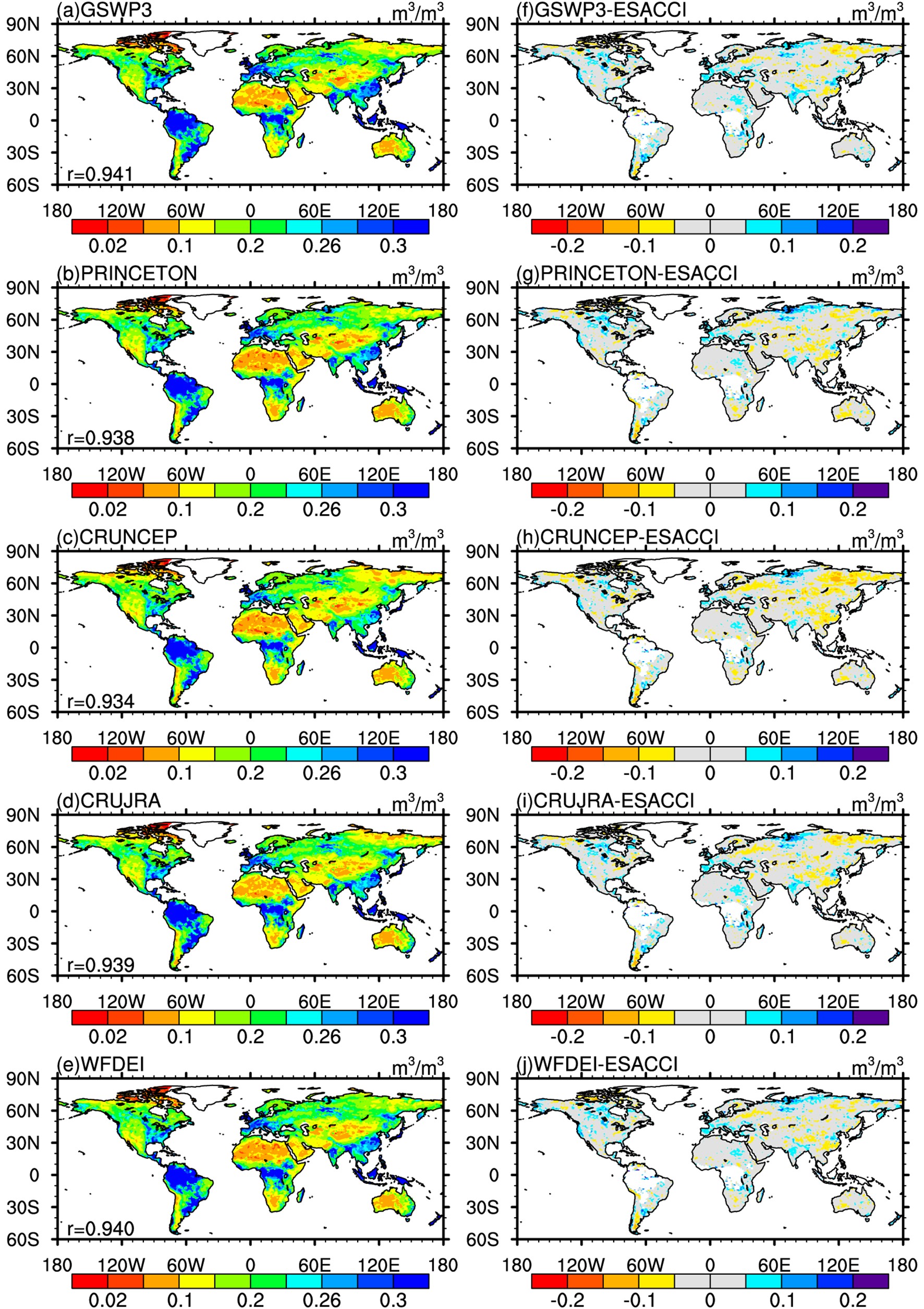 Figure1. The spatial patterns of surface soil moisture (top 10 cm) derived from five LMIP simulations (GSWP3, PRINCETON, CRUNCEP, CRUJRA, and WFDEI) and their differences with the ESA CCI soil moisture product between 1979 and 2010. r in the left column indicates the spatial correlation coefficient of the model-based simulations with ESA CCI.
As shown in Figs. 2a and 2b, the five LMIP simulations show significantly increasing trends in surface and root zone soil moisture during the past 36 years (1979?2014) due to significantly increased precipitation (Fig. 2c). Compared with the other four simulations, GSWP3 has the wettest surface and root zone soil moisture due to higher precipitation. In contrast, CRUNCEP shows the lowest soil moisture, which may be related to the lower precipitation (Fig. 2c) and higher temperature (Fig. 2d). Clear differences in soil moisture can be observed among the five LMIP simulations; however, they are mainly systematic biases and the temporal correlation coefficients for the five datasets are high (over 0.9), indicating that the five LMIP simulations have consistent temporal variations in soil moisture. Additionally, all five forcing data sets show similar spatial distributions of the air temperature (not shown), since they were all bias corrected to different versions of CRU products. In contrast, the annual precipitation shows some differences. WFDEI shows slightly larger precipitation than GSWP3 over most land areas, while CRUNCEP and PRINCETON shows lower values globally (Wang et al., 2020b). This is because the precipitation of GSWP3 and WFDEI was biased corrected to different versions of GPCC products with different approaches to under-catch correction while CRUNCEP, CRUJRA, and PRINCETON were bias-corrected to different versions of CRU products. Interannual variations in precipitation and the 2 m temperature are presented in Figs. 2c and 2d, respectively. The global mean land precipitation shows a consistent increasing trend (0.7?1.5 mm yr?1, p < 0.05) concurrent with a rapid warming trend (0.024°C yr?1?0.029°C yr?1, p < 0.05) in the five datasets.
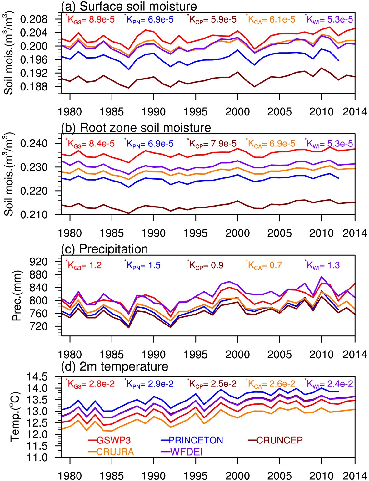 Figure2. Interannual variations of (a) surface soil moisture (top 10 cm), (b) root zone soil moisture (0?200 cm), (c) precipitation, and (d) 2 m temperature for the five LMIP simulations (GSWP3, PRINCETON, CRUNCEP, CRUJRA, and WFDEI) averaged globally (excluding Greenland) between 1979 and 2014. K is the trend for soil moisture (m3 m?3 yr?1), precipitation (mm yr?1), and temperature (°C yr?1) calculated using the Mann-Kendall test method; the subscript of K: G3 (GSWP3), PN (PRINCETON), CP (CRUNCEP), CA (CRUJRA), and WI (WFDEI). The asterisk represents the statistically significant trends (p < 0.05).
2
3.2. Snow
The changes in snow over the Northern Hemisphere (NH, poleward of 25°N) were examined using the satellite-based SCF. The climatological seasonal cycles in Fig. 3 were computed for 2001?2014, but only autumn (SON), winter (DJF), and spring (MAM) seasons were presented. In general, the SCF estimates from the five LMIP simulations capture the spatial patterns of the MODIS-derived SCF product well, with spatial correlation coefficients of over 0.957 for the three seasons. However, differences could be observed in the areas with complex terrain, for example, in the western United States, and on the Tibetan Plateau. This may be due to sub-grid scale snow variations, in complex terrain, not being accurately represented in the CAS-LSM, including blowing snow and the effect of aspect and slope on snow accumulation and melting (Xie et al., 2018b). The SCF is positively biased over the Tibetan Plateau, Alaska, and parts of western Siberia. In contrast, all five LMIP simulations tend to overestimate the SCF over most of the middle latitudes of Asia, Europe, and North America. In addition, there are larger positive biases over the high latitudes across the central and eastern United States and northern Europe during winter and spring. Detailed comparison results with ground measurements and satellite-based observations including SCF, snow depth, and snow water equivalent can be found in Wang et al. (2020b).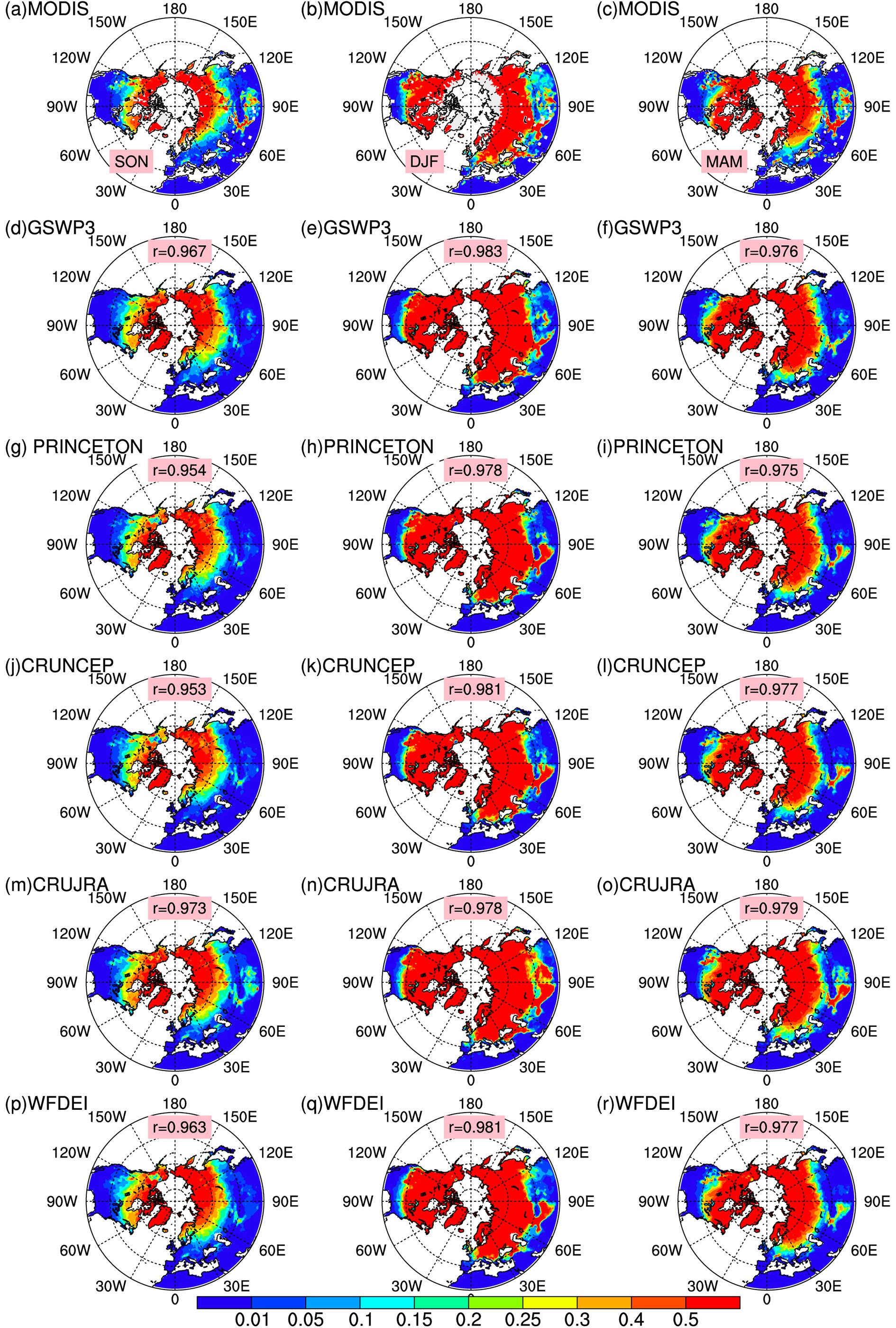 Figure3. Northern Hemispheric distributions of the mean seasonal snow cover fractions from (a?c) MODIS and (d?r) the five LMIP simulations during autumn (SON, left column), winter (DJF, middle column), and spring (MAM, right column) between 2001 and 2014. The r is the spatial correlation coefficient of the model-based simulations with MODIS.
2
3.3. Latent and sensible heat fluxes
We validated the spatial patterns of latent and sensible heat fluxes from the five LMIP simulations using the FLUXCOM product. All model simulations show acceptable agreement with the spatial variation of sensible heat flux from FLUXCOM (Fig. 4), with correlation coefficients ranging between 0.831 and 0.905. However, a systematic overestimation is observed over parts of the northern low latitudes and most of the Southern Hemisphere for PRINCETON (Fig. 4g), CRUNCEP (Fig. 4h), CRUJRA (Fig. 4i), and WFDEI (Fig. 4j). All five simulations exhibit lower sensible heat fluxes over the northern high latitudes than FLUXCOM. Simulations with GSWP3 appear to have sensible and latent heat fluxes that are generally higher across the globe than the other four simulations and FLUXCOM. As shown in Fig. 5, all LMIP simulations capture the spatial pattern of the latent heat flux very well, with spatial correlation coefficients around 0.96. Model simulations show slight underestimations over most of the globe. This is particularly visible over the northern parts of South America and southern Africa. In addition, some systematic overestimations are found over Australia and the Tibetan Plateau.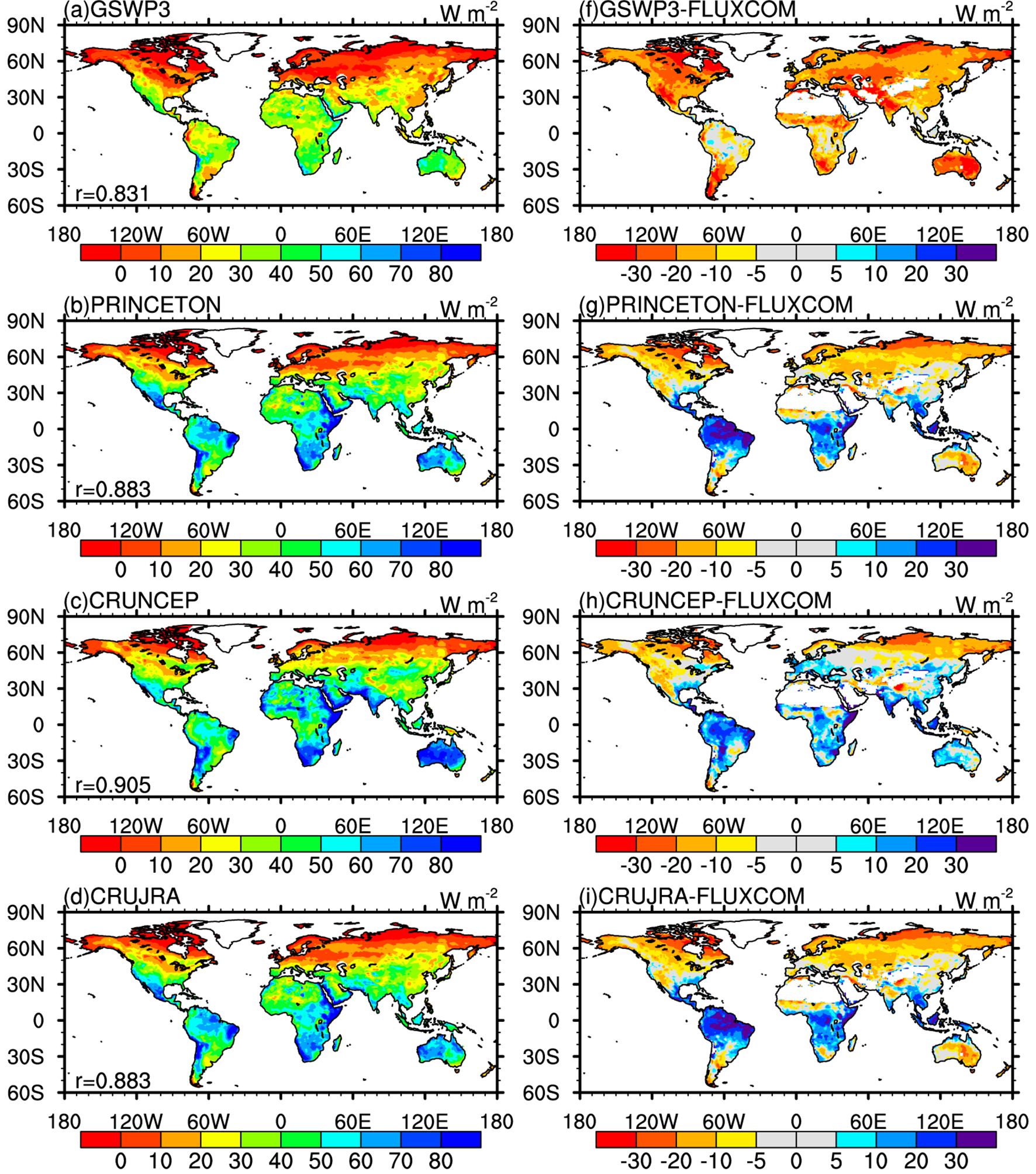 Figure4. Spatial patterns of sensible heat flux from the five LMIP simulations (GSWP3, PRINCETON, CRUNCEP, CRUJRA, and WFDEI) and their differences with FLUXCOM between 2001 and 2014. The r in the left column indicates the spatial correlation coefficient of the model-based simulations with FLUXCOM.
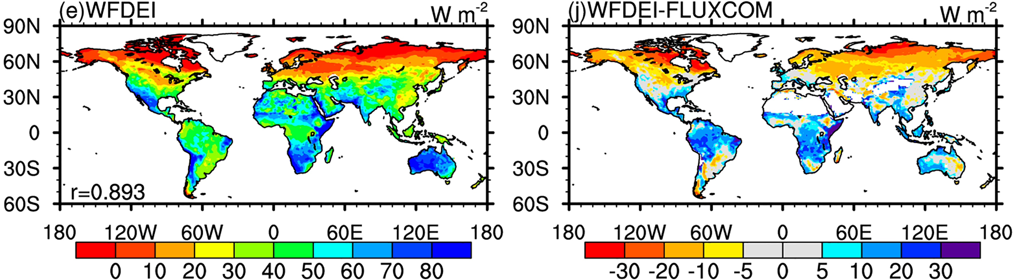 Figure4. (Continued)
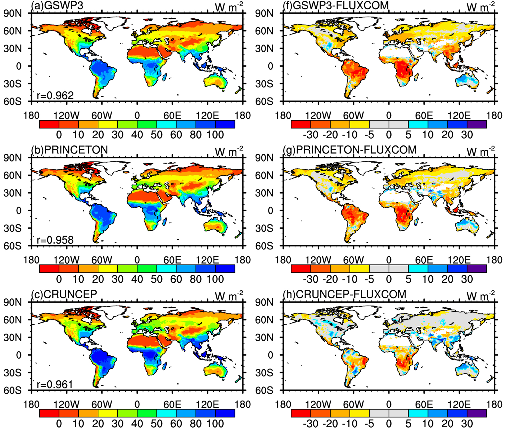 Figure5. Spatial patterns of latent heat flux from the five LMIP simulations (GSWP3, PRINCETON, CRUNCEP, CRUJRA, and WFDEI) and their differences with the FLUXCOM product between 2001 and 2014. The r in the left column indicates the spatial correlation coefficient of the model-based simulations with FLUXCOM.
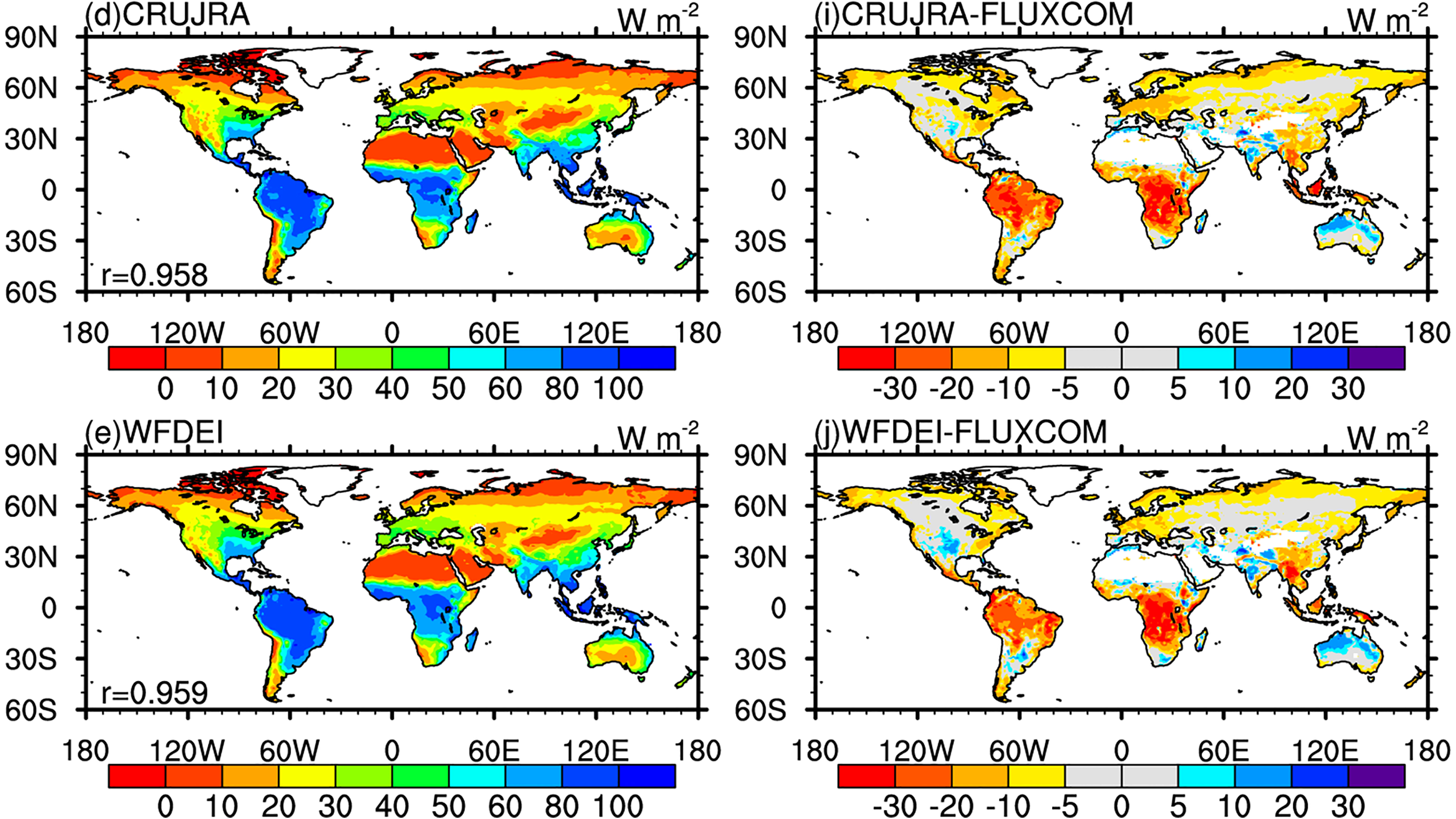 Figure5. (Continued)
2
3.4. Terrestrial water storage
TWS is the sum of water stored above and underneath the surface of the earth (Syed et al., 2008; Zeng et al., 2008) and plays an important role in Earth’s climate system (Zeng et al., 2008; Jia et al., 2020). The seasonal variations of TWSA from GRACE and five LMIP simulations for the period 2003?2014 are presented in Fig. 6. In general, the simulated seasonal patterns from CAS-LSM appear to be in good agreement with those from GRACE, with spatial correlation coefficients ranging between 0.40 and 0.72. In addition, “hot spots” with significantly negative TWSA values were present due to groundwater overexploitation (Rodell et al., 2009; Feng et al., 2013; Sinha et al., 2017; Wang et al., 2019), such as in northern India, the North China Plain, and the central United States. These negative anomalies were detected in both the GRACE observations and the model simulations for boreal winter, spring, and summer (Fig. 6). Figure6. Seasonal terrestrial water storage anomaly (TWSA) estimated using GRACE and simulated from the five LMIP simulations (GSWP3, PRINCETON, CRUNCEP, CRUJRA, and WFDEI) between 2003 and 2014. The r indicates the spatial correlation coefficient of the model-based simulations with GRACE.
The standard output of variables requested by LS3MIP (see
| Name | Long Name | Unit | Directiona | Dimb | Frequency |
| huss | specific humidity | kg kg?1 | ? | TYX | 3-hour |
| ps | surface air pressure | Pa | ? | TYX | 3-hour |
| rls | net longwave radiation | W m?2 | downward | TYX | daily |
| hfls | latent heat flux | W m?2 | upward | TYX | daily |
| hfss | sensible heat flux | W m?2 | upward | TYX | daily |
| tas | daily near?surface air temperature | K | ? | TYX | daily |
| tasmax | daily maximum near?surface air temperature | K | ? | TYX | daily |
| tasmin | daily minimum near?surface air temperature | K | ? | TYX | daily |
| ts | average surface temperature | K | ? | TYX | daily |
| pr | precipitation rate | kg m?2 s?1 | downward | TYX | daily |
| mrlsl | average layer soil moisture | kg m?2 | ? | TZYXc | daily |
| tws | terrestrial water storage | kg m?2 | ? | TYX | daily |
| mrro | total runoff | kg m?2 s?1 | out | TYX | daily |
| tran | vegetation transpiration | kg m?2 s?1 | upward | TYX | daily |
| et | total evapotranspiration | kg m?2 s?1 | upward | TYX | daily |
| gwt | groundwater extraction | mm s?1 | ? | TYX | monthly |
| a"Direction" identifies the direction of positive numbers. b"Dim" indicates the dimension of the variable. c"TZYX", T: time, Y: latitude, X: longitude, and Z: soil layers (15 layers). | |||||
Table2. Summary of the output data tables for the LMIP of LS3MIP derived from CAS-LSM of CAS FGOALS-g3
Acknowledgements. This work was supported by the Second Tibetan Plateau Scientific Expedition and Research Program (STEP) (Grant No. 2019QZKK0206), the Youth Innovation Promotion Association CAS, the National Natural Science Foundation of China (Grant No. 41830967), and National Key Scientific and Technological Infrastructure project “Earth System Science Numerical Simulator Facility” (EarthLab). We would like to thank the editors and three reviewers for their helpful comments that improved the manuscript.
The citation for LS3MIP of CAS FGOALS-g3 is “CAS FGOALS-g3 model output prepared for CMIP6 LS3MIP. Earth System Grid Federation.
The citation for land-hist-gswp3 is “CAS FGOALS-g3 model output prepared for CMIP6 LS3MIP land-hist. Earth System Grid Federation.
The citation for land-hist-princeton is “CAS FGOALS-g3 model output prepared for CMIP6 LS3MIP land-hist-princeton. Earth System Grid Federation.
The citation for land-hist-crujra is “CAS FGOALS-g3 model output prepared for CMIP6 LS3MIP land-hist-cruNcep. Earth System Grid Federation.
The citation for land-hist-wfdei is “CAS FGOALS-g3 model output prepared for CMIP6 LS3MIP land-hist-wfdei. Earth System Grid Federation.
The CRUNCEP simulations are available upon request. Please contact Binghao JIA at
The ESA CCI soil moisture data were downloaded from
Electronic supplementary material: Supplementary material is available in the online version of this article at
Open Access This article is distributed under the terms of the Creative Commons Attribution License which permits any use, distribution, and reproduction in any medium, provided the original author(s) and the source are credited. This article is distributed under the terms of the Creative Commons Attribution 4.0 International License (
