HTML
--> --> -->In recent years, concerns about the climate responses under the scenarios anchored by low warming targets (low warming scenarios) have motivated a large body of research and even the release of the special IPCC report on 1.5°C global warming after the 2015 Paris Agreement (IPCC, 2018; Li et al. 2018; Long et al., 2018, 2020; Nangombe et al., 2018; Palter et al., 2018; Qu and Huang, 2018; Zhang et al., 2018; Chen et al., 2019b). Previous studies imply that the spatial distributions and underlying mechanisms of the climate responses may be substantially different between low-forcing and high-forcing scenarios, as the low warming scenarios require much lower or even negative carbon emissions compared to that in the scenarios with moderate or no mitigation efforts (van Vuuren et al., 2011; IPCC, 2013, 2018; Sanderson et al., 2016; Xu and Ramanathan, 2017). This highlights that further studies are needed to deepen our understanding on the dynamics and uncertainty of climate changes under low warming scenarios.
In phases 5 and 6 of the Coupled Model Intercomparison Project (CMIP5 and CMIP6, respectively), the low-forcing scenario of the Representative Concentration Pathway (RCP2.6) and its updated version (Shared Socioeconomic Pathway, SSP1-2.6) are both categorized as low warming scenarios (Taylor et al., 2012; Eyring et al., 2016). In both RCP2.6 and SSP1-2.6, radiative forcing (RF) is designed to follow nearly the same pathway that first increases to a peak of 3 W m?2 around 2045 and then decreases to 2.6 W m?2 by 2100. Climate responses are substantially different between RF increasing and decreasing stages as the deep ocean warms persistently despite the RF decrease, and thus can significantly shape the trajectories of GMST and surface climate change (Long et al., 2018, 2020). Surface temperature is a key factor in ocean–atmosphere–land interaction, and its future change could greatly affect changes in regional precipitation (Xie et al., 2010; Huang et al., 2013; Long et al., 2016), atmospheric circulation (Ma et al., 2012), and even ocean circulation (Wang et al., 2015; Chen et al., 2019a). However, surface temperatures changes under the low warming scenario in the newly released CMIP6 outputs have not been well studied.
The present study mainly addresses this issue based on the outputs of the Flexible Global Ocean–Atmosphere–Land System (FGOALS) climate models participating in the CMIPs. The models are developed at the Institute of Atmospheric Physics (IAP)/State Key Laboratory of Numerical Modeling for Atmospheric Sciences and Geophysical Fluid Dynamics (LASG), Chinese Academy of Sciences. The FGOALS models in CMIP5 and CMIP6 respectively provide simulations under the RCP2.6 and SSP1-2.6 scenarios (Bao et al., 2013; Lin et al., 2013; He et al., 2019, 2020; Zhou et al., 2020). The state-of-the-art FGOALS models in CMIP6 display substantial improvement in model resolutions, parameterization of physical processes, and tuning method from their predecessor versions in CMIP5, with smaller climate drift and reduced model biases in simulated climatology, seasonal cycles, and climate variability (Guo et al., 2020; Li et al., 2020). It is important to compare the surface temperature changes in the latest two generations of the FGOALS climate models to gain insight into the climate responses and underlying mechanisms under low warming scenarios.
Therefore, in this study, the surface temperature changes simulated by the FGOALS models under the RCP2.6 and SSP1-2.6 scenarios in CMIP5 (FGOALS-g2 and FGOALS-s2) and CMIP6 (FGOALS-g3 and FGOALS-f3-L) are investigated. We show that there are substantial differences in the patterns of surface temperature change between the RF increasing and decreasing stages over the land, Arctic, North Atlantic (NA) subpolar region, and Southern Ocean. Besides, the pattern of regional surface warming displays striking differences between the two generations of FGOALS models, mainly due to model-to-model differences in the climatological surface temperature field. The surface temperature differences among models can result in large intermodel spread in regional climate responses through different processes like the ice-albedo feedback and Atlantic Meridional Overturning Circulation (AMOC) response. The important implication of this study is that improving the simulation of the surface temperature climatology is helpful in achieving reliable future projections under low warming targets.
The rest of the paper is organized as follows. Section 2 describes the model outputs and methods. Section 3 presents the global mean responses under the RCP2.6 and SSP1-2.6 scenarios. Sections 4 and 5 investigate the patterns of global and regional surface temperature change, respectively. Section 6 provides a summary, along with some further discussion.
2.1. Model outputs
The last two generations of climate system models developed at LASG-IAP are FGOALS2 and FGOALS3, including two parallel subversions in CMIP5 (FGOALS-g2 and FGOALS-s2) and three parallel subversions in CMIP6 (FGOALS-g3, FGOALS-f3-L and FGOALS-f3-H). A detailed description of the model configurations can be found in related literature (Bao et al., 2013; Li et al., 2013, 2020; Zhou and Song, 2014; Guo et al., 2020; Zhou et al., 2020). Only four subversions are analyzed in the present study, as outputs of FGOALS-f3-H are currently not available on the CMIP6 data portal. Each version of the FGOALS models configures a similar coupling framework including oceanic, sea-ice, and land components, with differences mainly in the atmospheric models. Detailed information on these components is provided in Table 1. Note that the FGOALS-g3 (FGOALS-f3-L) model is the updated version of the FGOALS-g2 (FGOALS-s2) model.| CMIP | Model | Component | |||
| Ocean | Sea ice | Atmosphere | Land | ||
| CMIP5 | FGOALS-g2 | LICOM2 | CICE4 | GAMIL2 | CLM3 |
| 360 × 196 | 128 × 60 | ||||
| 30 levels | 26 levels | ||||
| FGOALS-s2 | LICOM2 | CSIM5 | SAMIL2 | CLM3 | |
| 360 × 196 | 128 × 108 | ||||
| 30 levels | 26 levels | ||||
| CMIP6 | FGOALS-g3 | LICOM3 | CICE4 | GAMIL3 | CLM4 |
| 360 × 218 | 188 × 80 | ||||
| 30 levels | 26 levels | ||||
| FGOALS-f3-L | LICOM3 | CICE4 | FAMIL | CLM4 | |
| 360 × 218 | 288 × 180 | ||||
| 30 levels | 32 levels | ||||
Table1. Model components and corresponding horizontal resolutions of FGOALS models in CMIP5 and CMIP6. The components of all the models are the Finite-volume Atmospheric model (FAMIL), the Spectral Atmospheric Model of IAP/LASG (SAMIL), the LASG/IAP Climate system Ocean Model (LICOM), the Community Land Model (CLM), the Community Sea Ice Model (CSIM), and the Los Alamos sea ice model (CICE). The version number of the component models are labeled after the acronyms.
The equilibrium climate sensitivity (ECS), defined as the equilibrium temperature under doubled CO2 forcing, is 2.1–4.7 K in CMIP5 models and 1.8–5.6 K in CMIP6 models (Zelinka et al., 2020), which is mainly due to stronger positive cloud feedbacks from decreasing extratropical low-cloud coverage and albedo in models from CMIP6 than CMIP5. In contrast, the ECS is about 3.7 K in FGOALS-g2 and 4.5 K in FGOALS-s2, but decreases to 2.84°C for FGOALS-g3 and 2.98°C for FGOALS-f3 (Zhou et al., 2013, 2020), which might be associated with the differences in model biases and model-simulated internal variability, Arctic climate, and ocean circulation responses.
The ability of climate models in reproducing the climatology of observations, which is measured by the model bias (i.e., deviation from observation), is an essential metric for evaluating model performance. Figure 1 shows the spatial distribution of annual mean climatology biases in SST and 2 m air temperature (TAS) in FGOALS models for 1979–2005. The ERSST.v5 (Huang et al., 2017) and high-resolution (0.5° × 0.5°) CRU TS4.04 (Harris et al., 2020) data are referenced as observations to calculate the model biases. Generally, the FGOALS models display similar bias patterns in SST and TAS in both CMIPs, with large cold SST bias in the North Pacific, warm SST bias along the eastern coast of subtropical ocean basins and the Southern Ocean, and large cold TAS bias in Eurasia and North America. The maximal and minimal model biases in both SST and TAS also change insignificantly from CMIP5 to CMIP6. However, the global root-mean-square error (RMSE) and global mean value of SST biases are reduced in FGOALS from CMIP5 to CMIP6, with noticeable reduction in the North Pacific, south of Greenland, Southern Hemisphere (SH), eastern subtropical oceans, and Southern Ocean. For TAS bias, there is also a prominent decrease in its magnitude over western Eurasia, North America and Australia. Besides, the updated FGOALS models significantly reduce the TAS biases of their predecessors over regions along the Rocky and Andes Mountains and Himalayas, suggesting an improvement in resolving the effect of topography in CMIP6 models. As a result, the global RMSE and global mean value of TAS biases also decrease, especially for the latter. The evaluation of model biases in FGOALS models suggests that there are significant improvements and changes in the performances of FGOALS-g3 and FGOALS-f3-L from their predecessors.
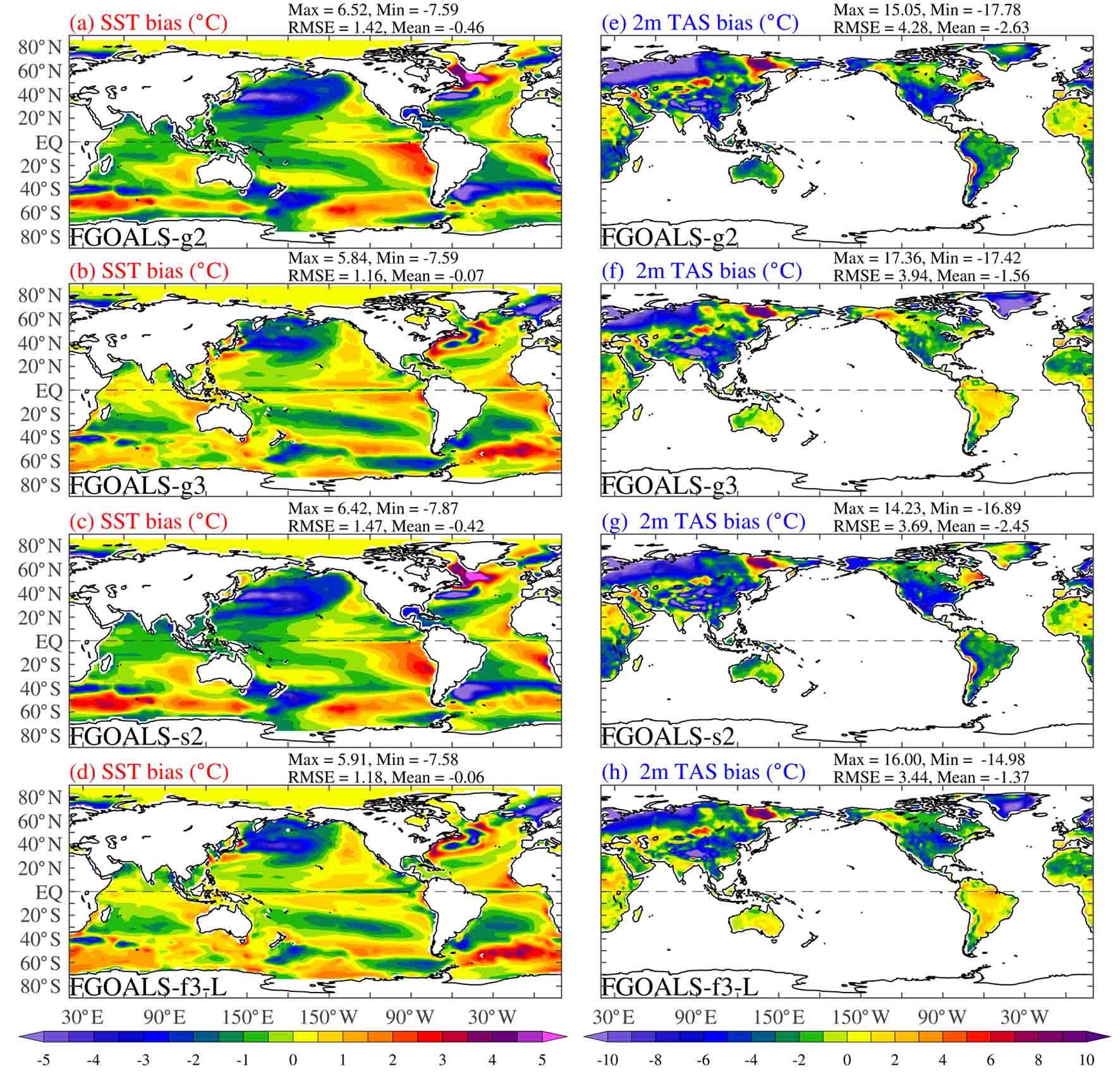 Figure1. Spatial distribution of annual mean biases in SST (units: °C) and 2 m air temperature (TAS; units: °C) in (a, e) FGOALS-g2, (b, f) FGOALS-g3, (c, g) FGOALS-s2, and (d, h) FGOALS-f3-L, during 1979–2005. The ERSST.v5 and CRU TS4.04 data are referenced as the observations. The maximum value (Max), minimum value (Min), RMSE, and mean value (Mean) of global biases are labeled at the top of each panel.
2
2.2. Methods
Monthly outputs (1850–2100) of historical simulations and low warming scenarios (RCP2.6 and SSP1-2.6) from the FGOALS models are analyzed. Besides, an additional 15 CMIP6 models (Table 2) are used to compare with their family predecessors in CMIP5. The CMIP5 and CMIP6 multi-model ensemble mean (MME) results are calculated based on the 15 pairs of models without the FGOALS models. The pre-industrial control runs are also used to remove the effect of climate drift in the models. Near-surface air temperature, surface temperature (skin temperature), precipitation, and zonal winds are used in this study. Note that in CMIP outputs, surface skin temperature is equivalent to SST in ice-free ocean. All atmospheric variables are linearly interpolated onto a common grid of 2° latitude × 2° longitude for ease of comparison. Only one member of each model is utilized for the analyses.| CMIP5 | CMIP6 | |
| 1 | BCC_CSM1.1(m) | BCC-CSM2-MR |
| 2 | CanESM2 | CanESM5 |
| 3 | CESM1-CAM5 | CESM2 |
| 4 | CNRM-CM5 | CNRM-CM6-1 |
| 5 | GFDL-CM3 | GFDL-ESM4 |
| 6 | GISS-E2-R | GISS-E2-1-G |
| 7 | HadGEM2-ES | HadGEM3-GC31-LL |
| 8 | IPSL-CM5A-LR | IPSL-CM6A-LR |
| 9 | MIROC5 | MIROC6 |
| 10 | MIROC-ESM | MIROC-ES2L |
| 11 | MPI-ESM-LR | MPI-ESM1-2-LR |
| 12 | MPI-ESM-MR | MPI-ESM1-2-HR |
| 13 | MRI-CGCM3 | MRI-ESM2-0 |
| 14 | NorESM1-M | NorESM2-LM |
| 15 | NorESM1-ME | NorESM2-MM |
Table2. CMIP models used in the present study.
As RF first increases to a peak around the year 2045 and then decreases, we separately calculate the linear trends during the RF increasing stage (1850–2050) and RF decreasing stage (2050–2100) to investigate the climate responses during these two distinct periods. The separation point for the trend calculation (2050) is chosen to lead lag the RF inflection point (2045) by only five years because the time scale of the fast response in the ocean mixed layer is 3–5 years (Held et al., 2010). The AMOC index is defined as the maximum value of the meridional stream function at 35°N in the Atlantic.
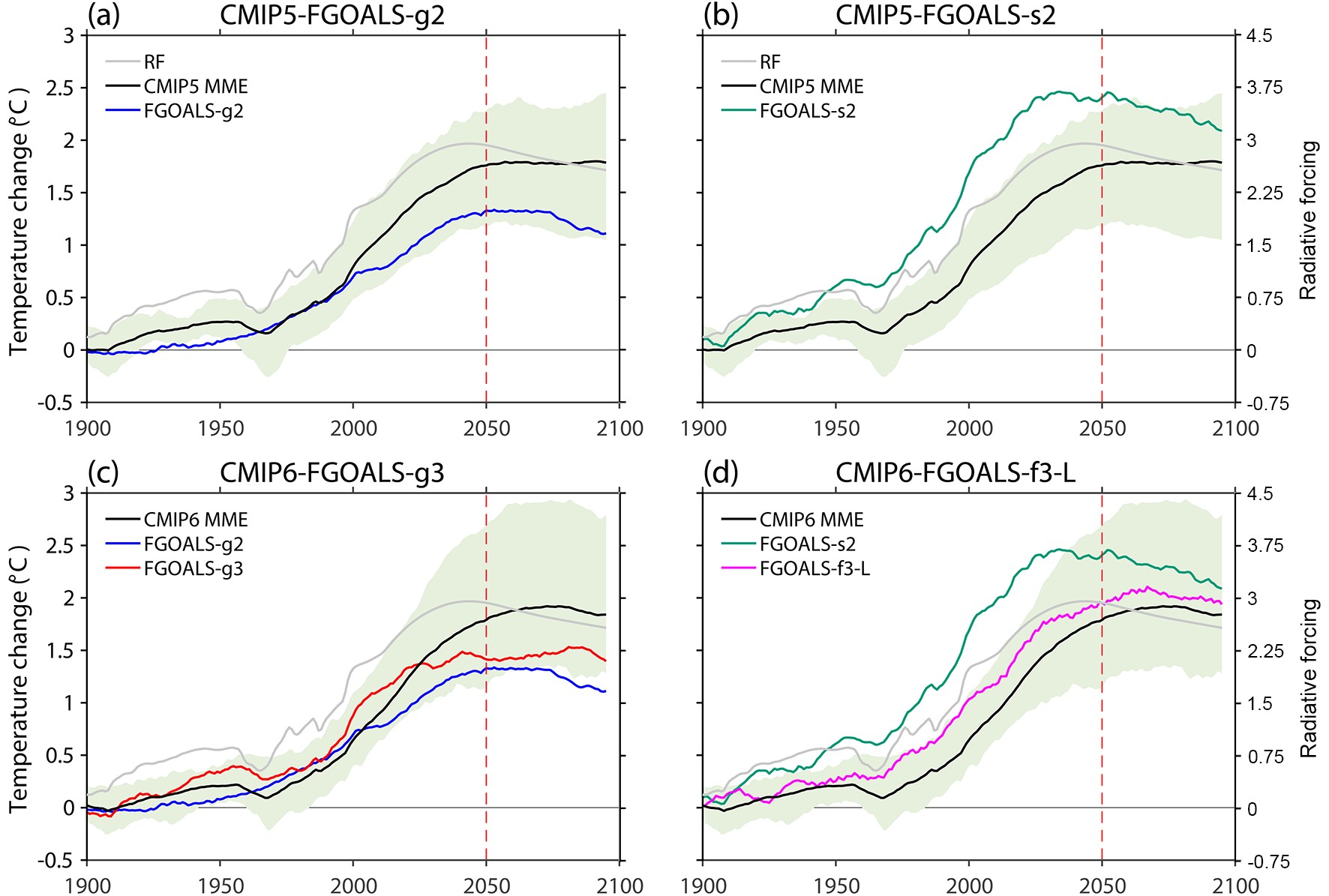 Figure2. Global mean annual surface air temperature change (units: °C) relative to pre-industrial level (1850–99 mean) in each FGOALS model (colored solid lines) and the CMIP5 and CMIP6 MMEs (black lines), with an 11-year running mean applied. The vertical dashed lines indicate the separation point for trend calculation. Note that the gray lines show the pathway of RF [right-hand axis in (b, d)], and the light green shadows indicate the range of the CMIP models.
During the RF decreasing stage (2050–2100), as discussed in previous studies (Long et al., 2018, 2020), the ratio between the contributions from fast and slow responses during the RF decreasing stage determines the further trend in GMST. This is because when RF ramps down, the ocean mixed layer would cool fast owing to rapid atmospheric cooling, hence lowering the GMST (fast cooling effect). In contrast, the deep ocean warms slowly but persistently through 2100 and thus reduces the downward heat transfer from the mixed layer, and this would additionally fuel the upper ocean warming and hence increase the GMST (slow warming effect). In both FGOALS-g2 and FGOALS-s2, the fast cooling effect outweighs the slow warming effect, leaving the GMST to slightly and sharply decrease (all significant) during 2050–2100, respectively. In FGOALS-g3 and FGOALS-f3-L, the fast cooling effect and slow warming effect nearly offset each other, leading to an insignificant trend in GMST during the RF decreasing stage, which is also a common feature in most CMIP5 models (Long et al., 2020).
The increase in GMST meets the 1.5°C warming target in FGOALS-g2 and FGOALS-g3, and is still below the 2°C warming level in FGOALS-f3-L. In FGOALS-s2, the increase in GMST exceeds 2.0°C after 2010 and maximizes at nearly 2.5°C. The large GMST increase in FGOALS-s2 is associated with a lack of the effect from direct aerosol cooling in the atmospheric model (Bao et al., 2013) and large ice-albedo feedback in the sea-ice model (CSIM5), which will be discussed in the next section.
The abovementioned features in GMST trajectories are more robust over land (red lines in Fig. 3) than ocean (green lines in Fig. 3) in all four models. The land–sea warming contrast (brown lines) also increases before 2050 and then decreases (Figs. 3a and b) or holds nearly constant (Figs. 3c and d) during 2050–2100, consistent with the GMST pathways (black lines). It is worth noting that the range of the CMIP models increases slightly after 2050, suggesting increased intermodel spread and hence model uncertainty during the RF decreasing stage.
 Figure3. Global mean annual surface air temperature change (units: °C) over ocean (green lines) and land (red lines) and their difference (land–sea warming contrast, brown lines) relative to the pre-industrial level (1850–99 mean), with an 11-year running mean applied.
Global mean responses under the low warming scenario suggest that the GMST trajectory may not follow the RF pathway when RF decreases, mainly due to the warming effect from the slow increase in deep ocean temperature (Long et al., 2020). This is also a common feature in FGOALS and other CMIP models (Fig. 2). As regional climate change will largely deviate from the global mean response, we further investigate the spatial pattern of surface temperature change under low warming scenarios in detail.
 Figure4. Linear trend of annual surface skin temperature (units: °C), which is equivalent to SST over ice-free ocean, during (a–d) 1850–2050 and (e–h) 2050–2100 in the four FGOALS models. The white (black) dots indicate the trend is insignificant (significant) at the 95% level. The global mean value is labeled in the title of each plot.
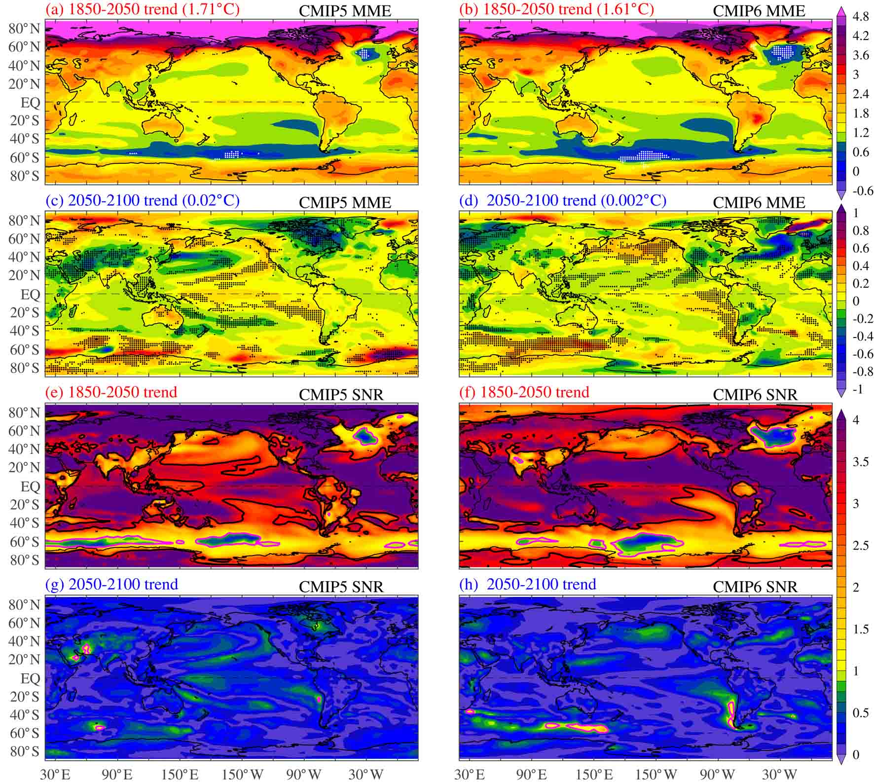 Figure5. MME linear trends of annual surface temperature (units: °C) during (a, b) 1850–2050 and (c, d) 2050–2100 in (a, c) CMIP5 and (b, d) CMIP6, along with (e–h) their SNRs, defined as the absolute value of MME change divided by the intermodel standard deviation. The magenta and black contours indicate SNRs of 1 and 3, respectively.
During 2050–2100, corresponding to the significant decreasing trend of GMST (Figs. 2a and b), the surface cooling pattern is prominent in FGOALS-g2 and FGOALS-s2. However, the cooling magnitude differs across regions and is mainly large in the tropics in FGOALS-g2 and in the Northern Hemisphere (NH) mid and high latitudes in FGOALS-s2. Despite the GMST change being negligible during 2050–2100 in these two CMIP6 models, there is still a significant cooling trend in the tropics and warming trend in the NH mid and high latitudes in FGOALS-g3, but overall weak temperature change in FGOALS-f3-L. Besides, there is a broad significant increasing trend in the Southern Ocean in both FGOALS-g3 and FGOALSf-3-L, which is missing in the CMIP5 FGOALS models. This suggest that ?TS may evolve prominently even under weak GMST change, but with the pattern differing significantly across models. It is worth noting that the ?TS patterns in the FGOALS models are generally consistent with the MME results during the RF increasing stage, with the global pattern correlation coefficients all exceeding 0.79 (Table 3). However, during the RF decreasing stage, the pattern consistency with the MME results drops dramatically, ranging from ?0.11 to 0.5 in the four models, suggesting that there is large model uncertainty in the further changes of surface temperature after 2050. In the CMIP5 and CMIP6 MMEs (Figs. 5c and d), the surface temperature mainly cools over land and warms over the SH oceans, but with the magnitude much reduced compared to that in the FGOALS models during 2050–2100 (Figs. 4e and f). Over the Tibetan Plateau, the surface cooling during the RF decreasing stage is also locally enhanced in most of the FGOALS models (Figs. 4e–g), and the CMIPs’ MMEs (Figs. 5c and d), which is similar to the situation during the RF increasing stage and suggests that the surface temperature over that region displays robust responses to RF changes.
| CMIP MME and models | Global | Tropical oceans | ||||
| 1850–2050 | 2050–2100 | 1850–2050 | 2050–2100 | |||
| CMIP5 MME | FGOALS-g2 | 0.86 | ?0.11 | 0.73 | ?0.21 | |
| FGOALS-s2 | 0.93 | 0.38 | 0.37 | 0.48 | ||
| CMIP6 MME | FGOALS-g3 | 0.79 | 0.50 | 0.80 | ?0.04 | |
| FGOALS-f3-L | 0.93 | ?0.02 | 0.59 | ?0.10 | ||
Table3. Pattern correlations between FGOALS models and their corresponding MME results. The bold values indicate that the correlations are significant at 95% confidence level.
To evaluate the role of model uncertainty, which is measured by the intermodel standard deviation (SD), in future projections, we further calculate the rate of model consistency in the sign of MME change and signal-to-noise ratio (SNR) in each grid cell. The former is measured by the rate of models displaying change with the same sign of the MME results and is shown in Figs. 5a–d, while the latter is defined as the absolute value of MME change divided by the intermodel SD and is shown in Figs. 5e–h. During the RF increasing stage, there is high model consistency in the sign of MME change across the globe, with a model consistency rate below 2/3 only appearing over a very limited area in the NA and Southern Ocean (white dots in Figs. 5a and b). The SNR is generally larger than 3 (black contours in Figs. 5e and f) over most regions during 1850–2050, indicating a robust MME change relative to its intermodel spread, and is only lower than 1 over the NA and Southern Ocean (magenta contours). During 2050–2100, the model consistency largely reduces over most regions, with consistent sign of change among models (black dots) mainly appearing over the Pacific subtropics and land regions with large surface cooling (Figs. 5c and d). Correspondingly, the SNR is much smaller than that during 1850–2050, with a very limited area displaying values larger than 1. The low model consistency and small SNR during the RF decreasing stage suggest that the intermodel spread is much larger than the MME change, which is inevitably associated with the intermodel differences in simulating the natural variability. During 2050–2100 (50 years), as the RF change is weaker and the length of time for trend calculation is much shorter than those during 1850–2050 (200 years), the interference of internal variability in the trend calculation rises consequently. Besides, the warming effect from the deep ocean slow warming also largely offsets the cooling effect from the RF decrease, especially over regions with strong ocean dynamics (Long et al., 2020). All these factors complicate the projections of the surface temperature changes during the RF decreasing stage. As a result, there are large intermodel differences in the ?TS pattern during 2050–2100, hence lowering the reliability of the MME changes. Indeed, during 1850–2050, the CMIP5 and CMIP6 MME ?TS patterns are highly similar, suggesting robustness of the projected surface temperature response to the increase in RF. During 2050–2100, despite the GMST change being insignificant in both CMIP5 and CMIP6, the ?TS pattern diverges substantially over the Arctic, East Asia, North America and NA Ocean.
Generally, surface temperature responses under low warming scenarios are distinct between the RF increasing and decreasing stages, and vary substantially across models, especially during the RF decreasing stage. Given that the pattern formation mechanisms for ?TS display large variations in space (Xie et al., 2010), we further investigate the ?TS pattern in the tropics and three other regions with noticeable local changes (the Arctic, NA subpolar region and Southern Ocean) in detail.
5.1. Tropical temperature and associated precipitation changes
Tropical SST plays a key role in regional and global climate, and is an important factor in typhoon/hurricane dynamics, atmospheric convection, and Hadley and Walker cells. The response of tropical SST to global warming is important because it could greatly affect changes in regional precipitation through the so-called “warmer-get-wetter” mechanism (Xie et al., 2010; Huang et al., 2013; Long et al., 2016). Specifically, tropical SST influences atmospheric convection mainly through the relative SST change, i.e., the deviations from tropical mean change, as the tropical convection threshold is mainly determined by the tropical mean SST (Xie et al., 2010; Ma et al., 2012). As a result, precipitation increases over regions with SST warming larger than the tropical mean warming, and vice versa. Note that as the tropical convection threshold also increases as global warming develops (Johnson and Xie, 2010), the relative SST change is defined by subtracting the tropical mean SST change over 30°S–30°N from the local SST change.Previous studies suggest that the “warmer-get-wetter” mechanism is prominent in explaining tropical precipitation changes because the dynamic effect from the slowdown of the Walker circulation (Held and Soden, 2006; Vecchi et al., 2006; Vecchi and Soden, 2007; Ma et al., 2012) would largely cancel the thermodynamic effect from the climatological precipitation distribution (Seager et al., 2010; Chadwick et al., 2013). The latter is the so-called “wet-get-wetter” mechanism (Chou and Neelin, 2004; Held and Soden, 2006; Chou et al., 2009). Therefore, we further investigate the patterns of relative SST change in the FGOALS models under RCP2.6 and SSP1-2.6.
Figure 6 shows the precipitation change (shading) and relative surface temperature change (?TS*, contours) in the tropical oceans during 1850–2050 and 2050–2100. All four models display an El Ni?o-like warming structure during 1850–2050, with positive ?TS* anchoring the increase in precipitation. In contrast, negative ?TS* prevails over the subtropics and leads to a decrease in precipitation in models except FGOALS-g3. The consistency in the ?TS* and precipitation change suggests that the “warmer-get-wetter” mechanism works well in FGOALS models.
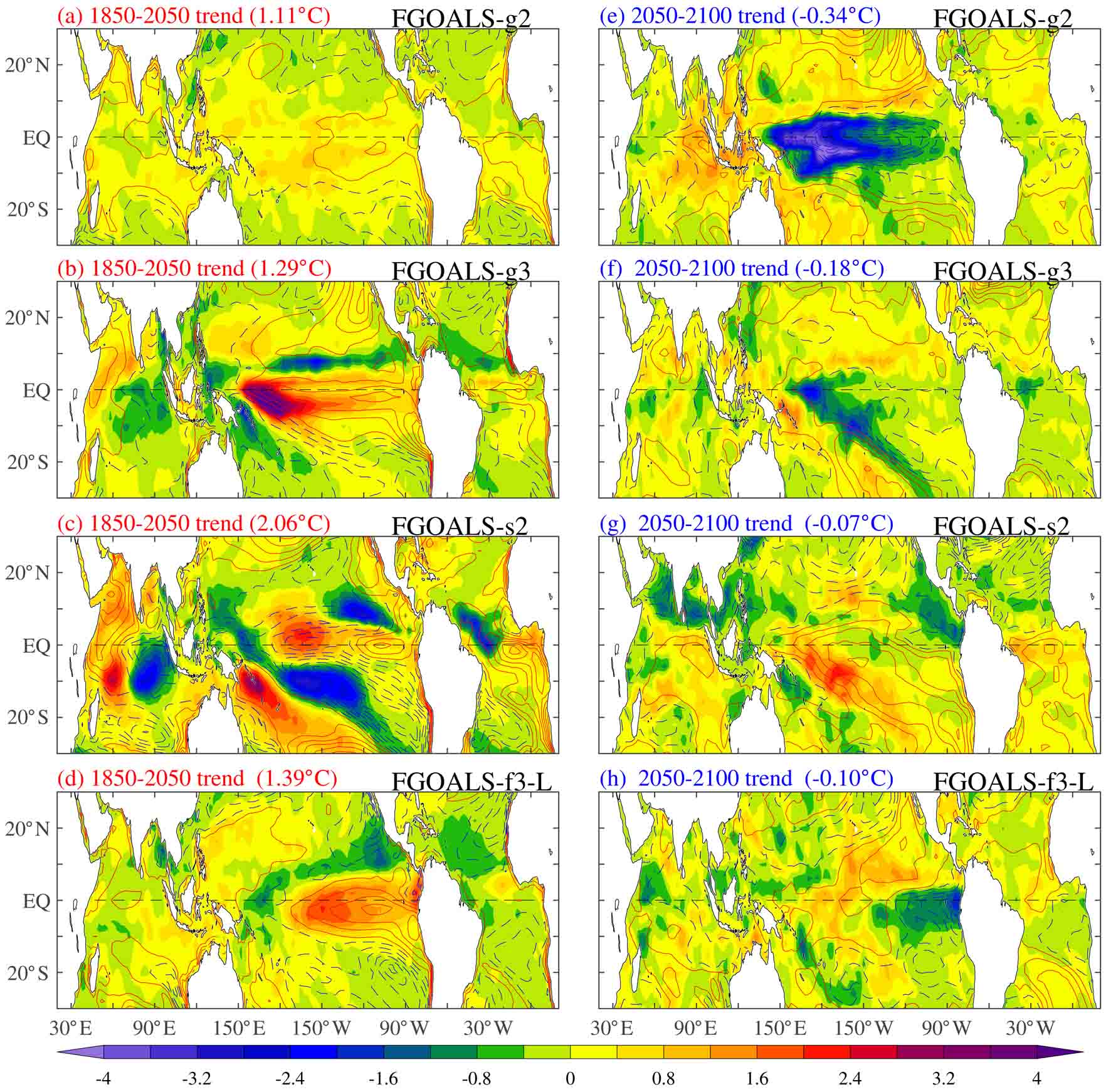 Figure6. Relative surface temperature change (?TS*, contours, interval = 0.15°C) and precipitation change (shading) in the tropical oceans during (a–d) 1850–2050 and (e–h) 2050–2100.
During 2050–2100, the tropical mean SST cooling is noticeable in FGOALS-g2 and FGOALS-g3 (Fig. 4e) but negligible in FGOALS-s2 and FGOALS-f3-L (Fig. 4f). The surface cooling spreads throughout the tropics in FGOALS-g2, especially in the equatorial Pacific, and the SH subtropics in FGOALS-g3, which also leads to a pronounced decrease in precipitation (Figs. 6e and f). However, precipitation still increases over several regions, mainly around the warm pool. This might be associated with the direct effect of the decrease in CO2 during 2050–2100. Previous studies have revealed that, in response to an increase in atmospheric CO2 concentration, global mean precipitation tends to decrease for several decades owing to fast tropospheric adjustment of the atmosphere, which is most prominent over the tropics because of Walker cell adjustment (Mitchell et al., 1987; Allen and Ingram, 2002; Lambert and Webb, 2008; Andrews et al., 2010; Wu et al., 2010; Kamae and Watanabe, 2013). Likewise, a decrease in atmospheric CO2 concentration would drive an increase in global mean precipitation and hence tropical circulation. Therefore, the effects from surface cooling and reduced CO2 jointly shape the pattern of tropical precipitation change during the RF decreasing stage. This is different from the case during the RF increasing stage, as the direct effect of increased CO2 on precipitation change is overwhelmed by the strong surface warming effect. Despite that the SST cools or weakly warms during the RF decreasing stage, the relative SST change still exerts strong control over the spatial structures in precipitation change in all FGOALS models (Figs. 6e–h). Precipitation generally increases or decreases slightly over regions with SST warming or SST cooling smaller than the tropical mean, and decreases substantially over regions with large SST cooling.
2
5.2. Arctic and Southern Ocean warming patterns
The pronounced Arctic warming (Arctic amplification) and reduced Southern Ocean warming are common regional patterns in all FGOALS models and CMIP MME results during the RF increasing stage (Figs. 4 and 5). The temporal evolutions of the area-weighted mean surface temperature over these regions are presented in Fig. 7.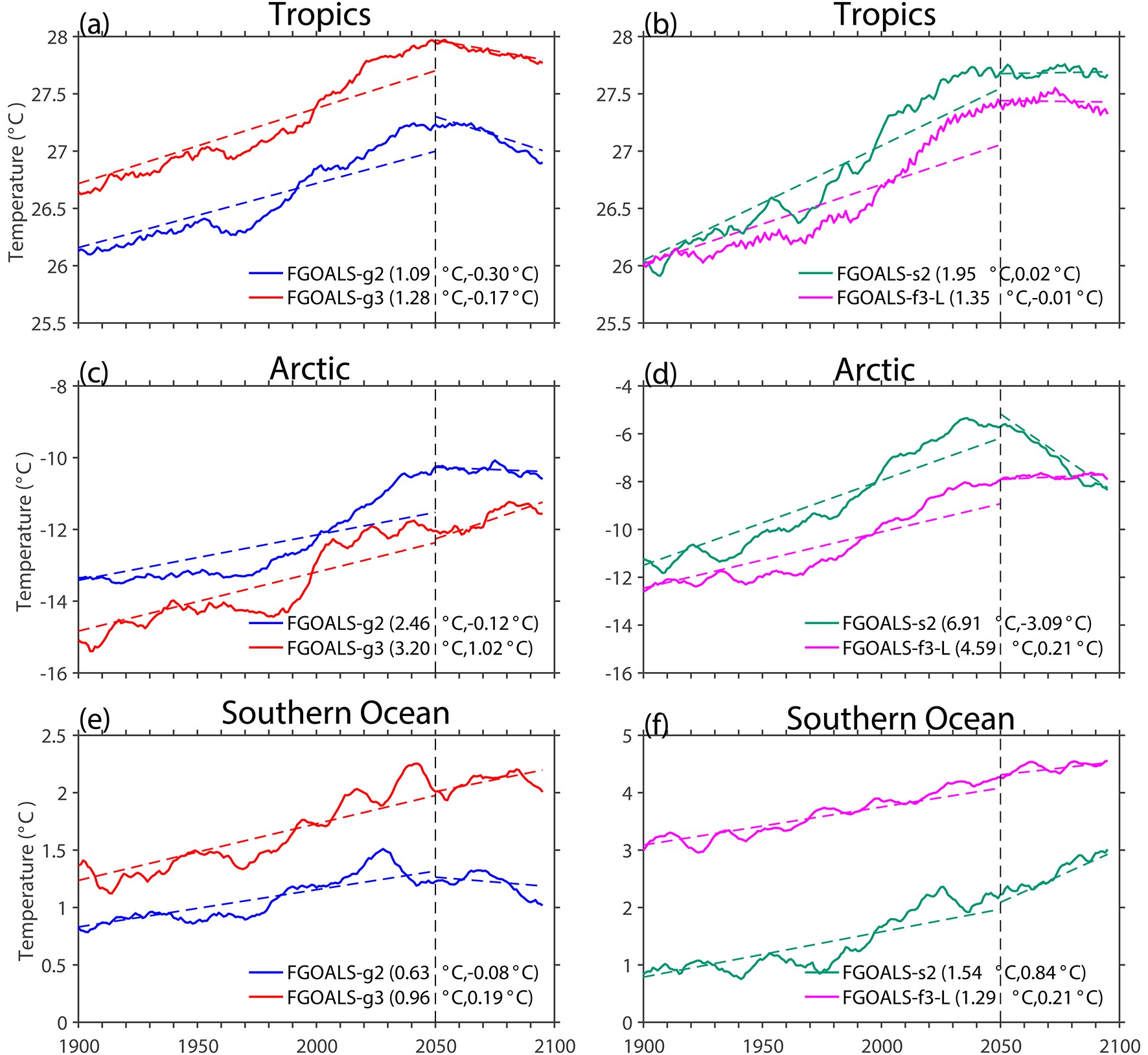 Figure7. Area-weighted mean annual surface temperature (units: °C) in the (a, b) tropical oceans (20°S–20°N), (c, d) Arctic (60°–90°N), and (e, f) Southern Ocean (65°–50°S), in FGOALS-g2 (blue lines), FGOALS-g3 (red lines), FGOALS-s2 (green lines), and FGOALS-f3-L (magenta lines), with an 11-year running mean applied. The colored dashed lines are the least-squares linear fitting lines for 1850–2050 and 2050–2100.
Arctic amplification is the most pronounced signal in the long-term climate change during recent decades and under future warming scenarios (Holland and Bitz, 2003; Serreze et al., 2009; Purkey and Johnson, 2010; Serreze and Barry, 2011; IPCC, 2013; Cohen et al., 2014). It involves or interacts with varies processes, including changes in atmospheric and oceanic circulation (Graversen et al., 2008; Chylek et al., 2009; Simmonds and Keay, 2009) and feedbacks associated with temperature in the low latitudes (Pithan and Mauritsen, 2014), cloud (Schweiger et al., 2008), water vapor (Francis and Hunter, 2007), snow, and sea ice (Winton, 2006; Kumar et al., 2010; Screen and Simmonds, 2010). Here, we mainly discuss the role of the ice-albedo feedback, which arises from the fact that ice has a much higher albedo and can reflect more solar radiation than land or water surfaces. An initial surface warming over ice surfaces would lead to ice melting and exposure of the underlying land or water to the atmosphere, and the reduced surface albedo that results would allow a greater absorption of surface heat. This enhances surface warming and leads to more ice melting, forming the positive feedback loop that is key in amplifying the initial Arctic surface temperature anomaly.
The climatological Arctic surface temperature is about 2°C–3°C colder in FGOALS-g2 and FGOALS-g3 than in FGOALS-s2 and FGOALS-f3-L by 1900 (Figs. 7c and d), suggesting that models with a cold Arctic surface tend to display a large ice thickness that is supposed to result in weak Arctic amplification (Holland and Bitz, 2003). The thick ice would require more heat for melting and hence delay the trigger and development of the ice-albedo feedback. As a result, during 1850–2050, the Arctic warming is much smaller in FGOALS-g2 and FGOALS-g3 than in FGOALS-s2 and FGOALS-f3-L. Indeed, the area-averaged annual mean ice thickness is 3.24 m for FGOALS-g2 and 1.81 m for FGOALS-s2 in the climatology (Song et al., 2014), confirming the relationship between surface temperature and ice thickness.
It is worth noting that the Arctic warming is the largest in FGOALS-s2, accompanied by the highest Arctic surface temperature in the climatology. As reported in Bao et al. (2013), there is a lack of the direct aerosol effect in FGOALS-s2. As aerosol emissions are largest in the NH, the cooling effect of aerosol would be underestimated in the NH, resulting a warmer Arctic surface and hence thinner ice in FGOALS-s2 than the other models. Therefore, the Arctic amplification is also the most prominent in FGOALS-s2, with a warming close to 7°C relative to the pre-industrial level by 2050. When RF decreases, the Arctic surface temperature displays a sharp decreasing trend of ?3°C during 2050–2100, which may be triggered by the shutdown of AMOC in FGOALS-s2, which is discussed in the next section. This suggests that the positive ice-albedo feedback is highly efficient in amplifying the initial temperature anomaly in the sea-ice model of FGOALS-s2. In contrast, the Arctic temperature continues to rise significantly in FGOALS-g3 during the RF decreasing stage, possibly because the thick ice has not melted too much over some regions during the RF increasing stage. In FGOALS-g2 and FGOALS-f3-L, further changes in Arctic surface temperature are relatively small and mainly follow the GMST pathways.
During the RF increasing stage, there is broad reduced surface warming (i.e., warming trend smaller than the global mean) at 65°S–50°S (Figs. 4a–d), and this is accompanied by robust strengthening of the westerlies south of 45°S in all four models (Figs. 8a–d), which would drive strong Southern Ocean upwelling and equatorward Ekman transport that jointly suppress the Southern Ocean surface temperature increase (Armour et al., 2016). As a result, the area-weighted-mean Southern Ocean surface temperature increases much slower than most other regions (Figs. 7e and f). During the RF decreasing stage, surface temperature decreases slightly in FGOALS-g2 but continues to increase in the other models, especially in FGOALS-s2 (green line in Fig. 7f). This is distinct from the GMST trajectory during that period. As discussed in previous studies (Held et al., 2010; Long et al., 2014, 2018, 2020), the deep ocean warms persistently despite the decrease in RF, and would additionally increase the surface temperature. In the Southern Ocean high latitudes, as the deep ocean gradually warms (Long et al., 2020), the seawater upwelled to the surface during the RF decreasing stage is also warmer than that during the RF increasing stage. This would weaken the cooling effect from the upwelling and thus fuel the further increase in surface temperature over the Southern Ocean.
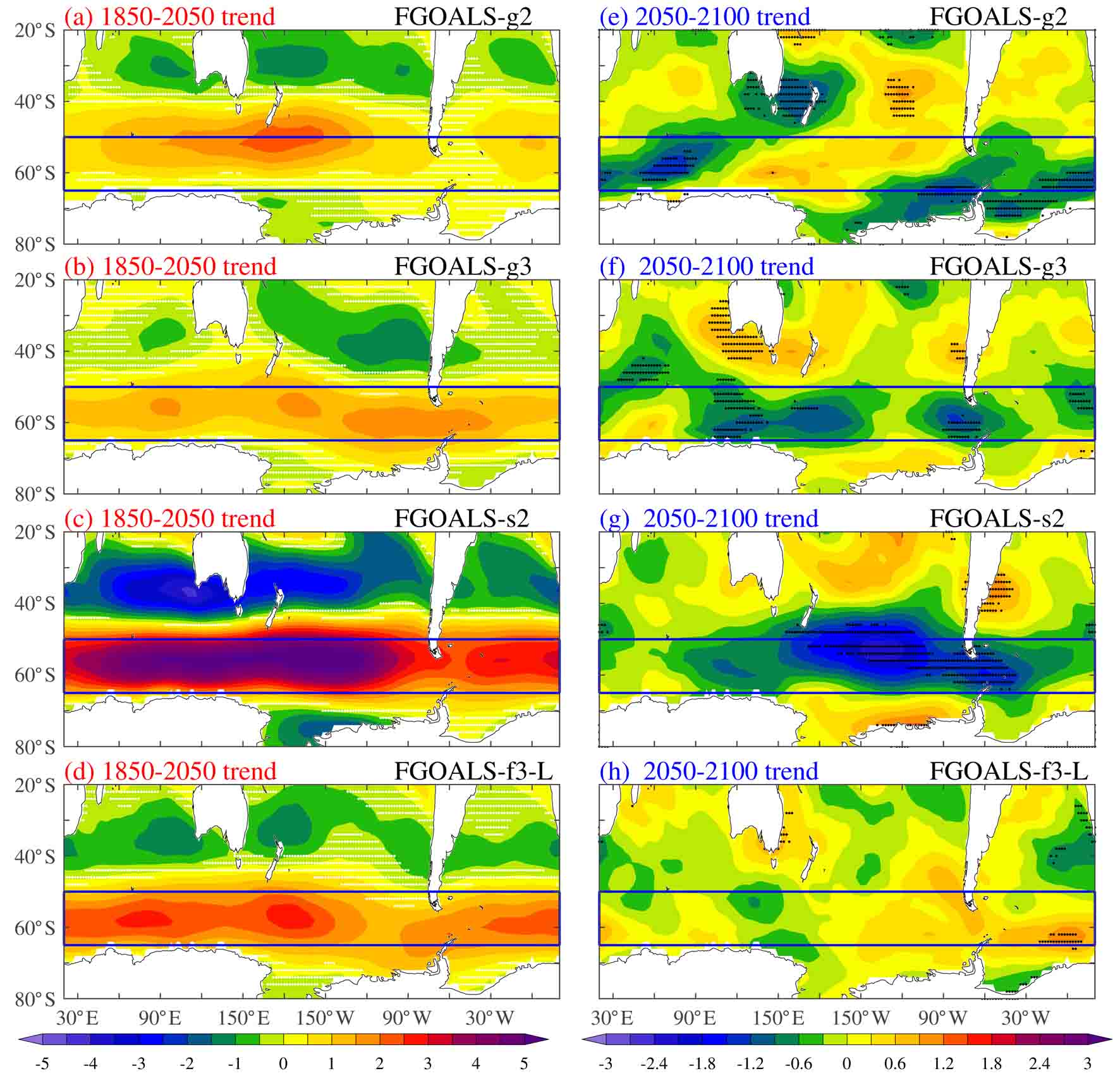 Figure8. Linear trend of annual 850 hPa zonal wind (units: m s?1) during (a–d) 1850–2050 and (e–h) 2050–2100 in the four FGOALS models. The white (black) dots indicate the trend is insignificant (significant) at the 95% level.
2
5.3. NA warming hole
The subpolar NA is a region of complex ocean dynamics. It plays a key role in regional and global climate variability at long time scales, such as Atlantic Multidecadal Oscillation (AMO), as the North Atlantic Deep Water (NADW) forms over there. Under global warming, the NA subpolar region features reduced surface warming relative to the global mean warming level, or even a cooling trend, in the 20th century, i.e., the NA warming hole (Drijfhout et al., 2012). This spatial structure is also evident in all four FGOALS models under low warming scenarios (Figs. 4a–d) and is common in CMIP models (IPCC, 2013; Sgubin et al., 2017). However, the NA warming hole appears at different locations in FGOALS models (blue boxes in Figs. 4a–d), mainly due to the differences in the NADW formation regions and responses of NA subpolar gyres.The NA subpolar region displays the largest SST anomaly in the spatial pattern of the AMO (Li et al., 2020). Mechanisms for the formation of the NA warming hole have been studied in recent decades, including the role of AMOC, subpolar gyre adjustment, and local convection change (Kim and An, 2013; Sgubin et al., 2017; Menary and Wood, 2018; Keil et al., 2020). All these factors are also directly related to the AMO, as the NA subpolar region is also a key region in the AMO. Figure 9 shows the area-weighted mean surface temperature change over the NA warming hole region and corresponding AMO index, defined as the detrended area-weighted mean SST anomaly over (0°–60°N, 80°W–0°), in each model. The warming hole indices display substantial decadal and multidecadal variability and hence a weak warming trend or even cooling trend in the FGOALS models. Indeed, the detrended warming hole indices correlate well with the AMO indices in all four models between 1850 and 2100, with correlation coefficients ranging from 0.53 in FGOALS-f3-L to 0.85 in FGOALS-g2. Therefore, in the FGOALS models, the AMO is important in influencing the surface temperature change over the NA subpolar region or the NA warming hole, which has not been well investigated in previous studies (Drijfhout et al., 2012; Kim and An, 2013; Sgubin et al., 2017; Menary and Wood, 2018) as it is hard to disentangle the causality of AMO and AMOC change.
 Figure9. Area-weighted mean annual surface temperature change (unit: °C) in the NA warming hole region (WH index), with an 11-year running mean applied. The regions are marked as blue boxes in Fig. 3, which are (45°–60°N, 65°–30°W) in FGOALS-g2 and FGOALS-g3 and (40°–60°N, 40°–10°W) in FGOALS-s2 and FGOALS-f3-L. The brown lines indicate the AMO index, defined as the detrended area-weighted mean SST over (0°–60°N, 80°W–0°). The change is calculated as the difference between pre-industrial control simulations and simulations from historical and future scenarios. The colored dashed lines are the least-squares linear fitting lines for 1850–2050 and 2050–2100.
It is worth noting that in FGOALS-g3, the NA warming hole index displays much larger temporal variations than in the other three models. This is because the FGOALS-g3 model greatly overestimates the AMO SST anomalies over the west of Greenland and the Labrador Sea in both the historical and pre-industrial control runs (Li et al., 2020). The large temporal variations in the warming hole index substantially affect the linear trend, as the inflection point (2050) for trend calculation is right in the valley of the AMO cold phase. This leads to a large cooling trend during 1850–2050 and substantial warming trend during 2050–2100 over the NA warming hole region.
In FGOALS-s2, the NA subpolar surface temperature cools rapidly from 2020 to 2100, mainly due to the rapid weakening of the AMOC (Fig. 10d), which is absent in the other three models. The reduced northward heat transport due to the AMOC slowdown would lead to large cooling over the NH, which may trigger the ice-albedo feedback to cause remarkable Arctic cooling during 2050–2100, consistent with the results in Fig. 7d. Furthermore, the AMOC is nearly shut down in FGOALS-s2, mainly because of the large freshwater input over the NA subpolar regions from the striking Arctic warming-induced ice melting. The AMOC displays large intensity in the climatology (values labeled in the legend for Figs. 10c and d), and hence is more stable under external forcing in the other three models than in FGOALS-s2. Climatologically, the AMOC intensity is directly related to the surface temperature over the NA subpolar region, as cold surface water promotes deep water formation, and vice versa. In addition, from CMIP5 to CMIP6, the FGOALS models largely reduce the warm SST biases south of Greenland (Figs. 1a–d) and hence increase the climatological AMOC intensity (Figs. 10c and d). This further highlights that to achieve reliable AMOC projections under future warming scenarios, improving the model ability in reproducing the observed climatological SST over the NA subpolar region is the key. The surface temperature over the NA subpolar regions may also work as a useful “emergency constraint” in correcting AMOC projections in climate models, as the period of direct AMOC observations is rather short.
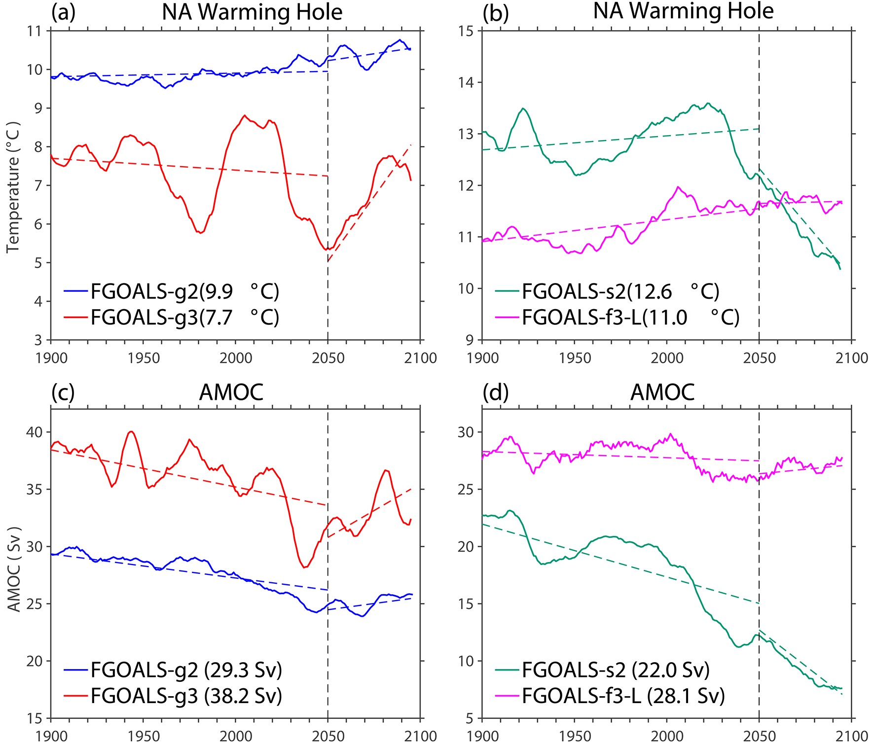 Figure10. Area-weighted mean annual surface temperature (unit: °C) in the (a, b) NA warming hole region and (c, d) AMOC index (unit: Sv), with an 11-year running mean applied. Note that the curves display the annual mean AMOC index in each year, but not the AMOC change. The colored dashed lines are the least-squares linear fitting lines for 1850–2050 and 2050–2100.
Furthermore, our results show that surface warming patterns are distinct between the RF increasing and decreasing stages, and display large differences across models. The most prominent differences appear over the land, Arctic, NA subpolar region, and Southern Ocean. The pattern consistency between the surface temperature change projected by the FGOALS models and the MME results is high during the RF increasing stage but low during the RF decreasing stage. This is mainly due to the relative short period for trend calculation in the latter, i.e., the natural variability plays an important role in obscuring the externally forced change during that period. Indeed, the CMIP5 and CMIP6 MMEs also display large differences over the NH mid and high latitudes during the RF decreasing stage, suggesting large model uncertainty in projecting the climate responses under weak GMST change. Tropical precipitation change is mainly anchored by the relative sea surface warming pattern during the RF increasing stage, which is a common feature in the FGOALS models. The relative SST change also exerts strong control over the pattern of precipitation change during the RF decreasing stage in all FGOALS models despite them displaying broad SST cooling or weak SST warming in the tropics.
The important implication of the present study is that by comparing the surface temperature responses in different FGOALS models, the diversity in the projected surface temperature change across models can largely be traced back to the intermodel differences in climatological surface temperature. In the Arctic, models with a warmer surface temperature would result in thinner ice and hence more active ice-albedo feedback and larger Arctic warming during the RF increasing stage than in the other models. The shutdown of AMOC in FGOALS-s2 is suggested to be tightly associated with the striking Arctic amplification-induced freshwater forcing over the NA subpolar region. Besides, the surface temperature over the NA subpolar region determines the magnitude of deep water formation and hence climatological AMOC intensity. Therefore, intermodel differences in NA subpolar climatological SST could lead to distinct AMOC responses and associated climatic effects globally across models in the future. Moreover, in the tropics, a 0.5°C difference in climatological SST could lead to substantially different patterns of precipitation change across the FGOALS models (Fig. 6). Consequently, a more realistic climatological surface temperature field is essential in reducing the intermodel spread of model-projected future changes, especially under low warming scenarios, where the RF is relatively weaker than under medium- and high-emissions scenarios. Further studies are needed to systematically investigate the detailed process involving the surface temperature changes under low warming scenarios in the state-of-the-art climate models from CMIP6.
Throughout the analyses of projected future surface temperature changes under low warming scenarios, we can see striking differences between both global mean and regional changes from the four FGOALS models during both the RF increasing and decreasing stages. Such differences across models might be associated with complicated process, such as the differences in model biases, cloud simulation, RF data (Nie et al., 2019), AMOC stability, land and sea-ice models, and parameterization schemes. For example, the ECS is substantially reduced in the updated FGOALS models compared to their predecessors, which may relate to the improved simulation in climatological surface temperature, especially in terms of the warm bias over the Arctic and the NA subpolar region and cold bias over land. The model-simulated natural variability is also an important factor influencing the intermodel spread in future projections. As shown in Fig. 9, the magnitude and phase transition of the AMO differ substantially across the FGOALS models, which may involve the intermodel differences in climatological SST over the NA subpolar gyre, storm track, and climate feedbacks, etc. It is worth noting that, despite the locations of the NA warming hole being nearly identical in models from the same group (i.e., FGOALS-g2 and FGOALS-g3, FGOALS-s2 and FGOALs-f3-L), the temporal evolution of the warming hole and AMOC indices are distinct, especially during the RF decreasing stage, and display large multidecadal variability that is dominated by the AMO. As GMST stabilizes during the RF decreasing stage, model-to-model differences in simulating the coherent natural variability mode would lead to substantially different trend changes due to the relatively short period and relatively weak RF change. Therefore, improving the ability of climate models to reproduce the natural variability mode will help to improve the reliability of model-projected future change under low warming scenarios.
Acknowledgements. We acknowledge the WCRP Working Group on Coupled Modeling, which is responsible for CMIP, and the climate modeling groups for producing and making available their model outputs. All data are available at
