HTML
--> --> -->Although the Antarctic Peninsula has more research stations compared to the rest of the Antarctic continent, several meteorological stations are underused due to a lack of archiving and complete time series (Lazzara et al., 2012; Fraiman et al., 2014). This is an impediment to expanding our knowledge of the climate variability of the peninsula. In particular, the Antarctic Peninsula cordillera constitutes an orographic obstacle to the westerlies, and thus the peninsula presents two different climatic zones: a relatively mild and humid marine climate on the west coast (windward), where northwesterly winds prevail, and a cooler continental climate on the east coast (leeward) (Fig. 1) mainly affected by southerly winds (King and Turner, 2009). The steep terrain of the Antarctic Peninsula, therefore, results in harsh conditions that further prevent the deployment of extensive field observations to obtain long-term records. On the one hand, with the aid of few available long-term surface meteorological records, the Antarctic Peninsula is considered to be one of the most vulnerable climate change ЁАhotspotsЁБ with a long-term warming trend in near-surface temperature observed over the last 50 years [e.g., Faraday/Vernadsky station, 2.94ЁуC (50 yr)?1] (Marshall et al., 2006; Turner et al., 2016, Jones et al., 2019). However, since the late 1990s, a cooling period has been observed in the Antarctic Peninsula that is attributed to atmospheric teleconnections (Carrasco, 2013; Turner et al., 2016; Oliva et al., 2017). On the other hand, a sparse observation network prevents extensive analyses to minimize the regional-scale uncertainties associated with climate variability and trends. Excluding the relatively short time series of satellite products, one common method of overcoming the difficulties arising from the inadequate observational network is to use gridded atmospheric data at high temporal resolution (i.e., reanalysis data) and/or high spatial resolution regional climate models (RCMs) to represent the main surface climatic features as well as to explore physical mechanisms behind the observed changes.
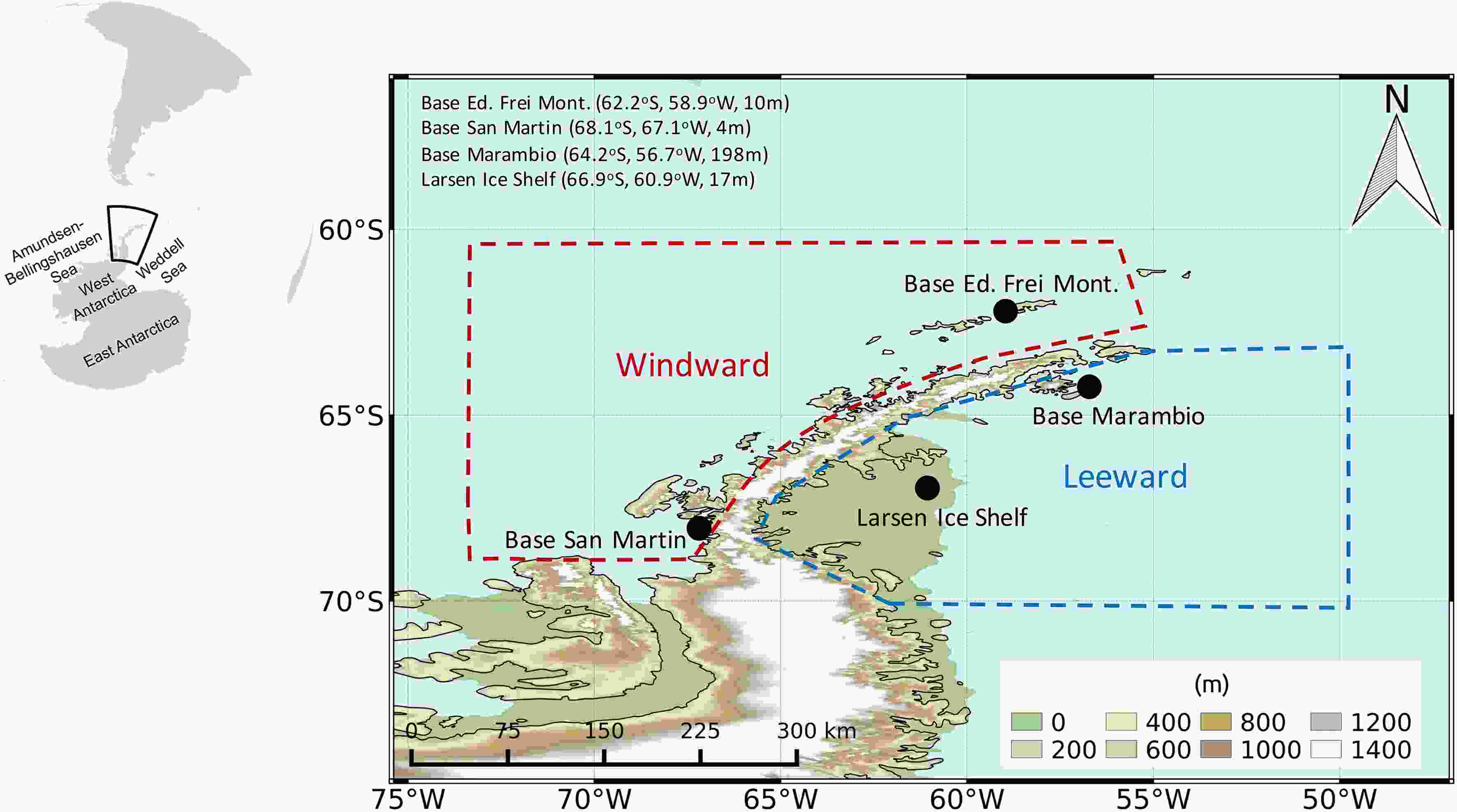 Figure1. Study region of the Antarctic Peninsula and meteorological stations (in black) used for the temperature analysis. The red and blue dashed lines correspond to the windward and leeward sides of the peninsula, respectively.
In recent years, atmospheric reanalysis data have been widely used for various studies such as surface climate characteristics of the Antarctic region as well as large-scale atmospheric forcing mechanisms modifying the surface climate variables. In a recent study, Gossart et al. (2019) performed a comprehensive comparison and evaluation of different reanalysis products in representing the surface climatology of the Antarctic Ice Sheet. They demonstrated that, although the reanalysis products could be useful tools, they can perform very differently depending on the region of interest, season and variable. Regarding the interplay between the local- and large-scale climate in the Antarctic continent, Hosking et al. (2013) investigated the Amundsen/Bellingshausen Sea low (hereafter ASL) using reanalysis data, and constructed diagnostic indices (i.e., the strength and location of the ASL). Also, Hosking et al. (2013) highlighted that the ASL is an important synoptic system modulating the West Antarctic climate variability. In another study, with the aid of reanalysis data, Rondanelli et al. (2019) highlighted the role of tropical variability in connection with the highest temperature recorded on continental Antarctica and associated large melting events over the Antarctic Peninsula.
In addition to surface observations and reanalysis products, a number of regional weather and climate model simulations have been employed over the Antarctic continent, particularly over West Antarctica and the Antarctic Peninsula. These modeling studies mainly consisted of the dynamical downscaling of boundary conditions provided by reanalysis, and covered a broad of spectrum of applications such as surface mass balance analysis (Lenaerts et al., 2012; van Wessem et al., 2014; Gonzalez et al., 2018; Agosta et al., 2019), characterizing surface climate patterns and variability (van Wessem et al., 2015; Deb et al., 2018), and foehn events (Steinhoff et al., 2014; Elvidge et al., 2015; Bozkurt et al., 2018; Datta et al., 2019; Zou et al., 2019).
Although the aforementioned efforts based on different data sources have helped to improve our understanding of the local-, regional- and large-scale climate variability of the Antarctic Peninsula, there is still a general lack of multiple-data source comparison and evaluation efforts that combine observed, reanalysis and RCM data. This is important for assessing and minimizing uncertainties and possible errors of interpreting the data arising from using a single data source. In particular, analyzing the recent spatiotemporal contrasts of temperature trends over the Antarctic Peninsula using multiple-data sources is crucial for accurately interpreting the climate variability of the region.
The main objective of the present study is, therefore, to investigate recent (1991?2015) near-surface temperature trends of the Antarctic Peninsula by combining observed, reanalysis and RCM data. Given the different climate characteristics of the peninsula on the windward and leeward sides of the cordillera, we first analyze the available near-surface temperature records to demonstrate trend differences on both sides. Then, we use the ECMWFЁЏs ERA5, and its predecessor ERA-Interim, for further analysis and comparison. Finally, we use hindcast simulations performed with the Polar-WRF (v3.9.1) RCM forced with ERA-Interim over the Antarctic Peninsula on a nested domain configuration at 45 km and 15 km spatial resolutions for the period 1991?2015. To our knowledge, this is the first complete high-resolution long-term simulation (> 20 years) including all seasons performed with Polar-WRF focusing on the Antarctic Peninsula. In addition, we include hindcast simulations of the KNMI-RACMO21P model forced with ERA-Interim obtained from the CORDEX-Antarctica domain at a spatial resolution of 50 km for further comparison. This allows us to contrast the changes in ERA5 and its predecessor ERA-Interim as well as the comparison of dynamical downscaling simulations with the boundary conditions from ERA-Interim. Section 2 describes the observed data, reanalysis and numerical simulations. Results are presented in section 3. Section 4 summarizes the results and presents concluding remarks.
2.1. Meteorological stations
We use four temperature observations located in the central and northern section of the Antarctic Peninsula (see Fig. 1). Eduardo Frei Montalva Base (Frei station) is the largest Antarctic base of Chile located at Fildes Peninsula near the northern tip of the Antarctic Peninsula. The data is provided by the Chilean National Weather Service (DirecciЈЎn MeteorolЈЎgica de Chile, DMC). Another station used in the northern tip of the peninsula is the Argentine Marambio Base. Although only ~250 km away from Frei station, it has a different climate as it is located on the leeward side of the northern peninsula (see section 3.1). In a similar manner, we use two more stations located in the center of the peninsula: the San Martin Base of Argentina on the windward side and the Larsen Ice Shelf station operated by the University of Wisconsin-Madison and the British Antarctic Survey on the leeward side. It should be noted that other weather stations are also available near the San Martin station; namely, Rothera and Faraday/Vernadsky stations. These two stations have already been extensively used in previous studies (e.g., Marshall et al., 2006; van Wessem et al., 2015; Turner et al., 2016); therefore, we use San Martin station, which has received less attention in the literature. On the leeward side, Esperanza station could also be used; however, Marambio station is located on the more leeward side about 100 kilometers southeast of Esperanza station, and is therefore more representative of the leeward conditions over the northern tip of the peninsula.The monthly data from the Marambio, San Martin and Larsen Ice Shelf stations are provided by the Scientific Committee on Antarctic Research (SCAR) Reference Antarctic Data for Environmental Research (READER; Turner et al., 2004) manned stations (San Martin and Marambio) and automatic weather station (Larsen Ice Shelf). Given the difficulties of finding a complete long-term record in the region, we use 1991?2015 as the period for the analysis. This period is also chosen to have a common period consistent with the RCM simulations (see section 2.3). We focus on the annual as well as summer (December?January?February, DJF) and autumn (March?April?May, MAM) time scales, as both large- and local-scale events can cause temperatures to rise above freezing, resulting in surface melting during these seasons (e.g., Nicolas et al., 2017; Bozkurt et al., 2018; Carrasco, 2018; Zou et al., 2019). Note that Larsen Ice Shelf station includes a low percentage of observations between 1990 and 1995 to perform the analysis; therefore, we have omitted the data between those years for this station. For station-based comparisons, temperature fields from gridded products (reanalysis and numerical simulations) are corrected using a constant lapse rate of 0.65ЁуC (100 m)?1 when there is a considerable elevation difference.
2
2.2. Reanalysis
We use monthly near-surface air temperature, mean sea level pressure, 850-hPa specific humidity and wind from the ECMWFЁЏs ERA-Interim reanalysis dataset (Dee et al., 2011) in order to present recent changes in surface and large-scale circulation patterns. The data assimilation system used to produce ERA-Interim is based on a 2006 release of the IFS (Cy31r2). The system includes a 4D variational analysis with a 12-h analysis window. The ERA-Interim data assimilation and forecast suite produces: (i) four analyses per day, at 0000, 0600, 1200 and 1800 UTC; and (ii) two 10-day forecasts per day, initialized from analyses at 0000 and 1200 UTC (Berrisford et al., 2011). The spatial resolution of the dataset is approximately 80 km (T255 spectral) on 60 vertical levels from the surface up to 0.1 hPa.In this work, we also include the ERA5 reanalysis, which is the most recent reanalysis product of the ECMWF and an updated version of ERA-Interim that combines large amounts of historical observations into global estimates using advanced modeling systems and data assimilation (C3S, 2017). ERA5 uses a more recent and improved version of the IFS Earth System Model and associated observational assimilation system [Cy41r2; Hersbach and Dee (2016)]. ERA5 has a globally improved spatial and vertical resolution on a 0.28Ёу ЁС 0.28Ёу (~30 km) grid and resolves the atmosphere using 137 levels from the surface up to 0.01 hPa (~80 km). ERA-Interim has recently been replaced by the ERA5 reanalysis. The reanalysis data extend from 1950 to the present, and we use the period 1991?2015 for the analysis. In the same way as ERA-Interim, we use monthly near-surface air temperature, mean sea level pressure, 850-hPa specific humidity and wind components from ERA5. This allows us a multi-comparison of reanalysis products as well as dynamically downscaled simulations versus their boundary conditions (ERA-Interim) and the new ERA5 reanalysis. A summary of the observations and reanalysis products used in this study are given in Table 1.
| (a) Meteorological Stations | ||||
| Data | Source | |||
| Stations | SCAR-READER, Chilean | |||
| Meteorological Service | ||||
| (b) Reanalysis Products | ||||
| Data | Source | Spatial resolution | Vertical levels | |
| ERA5 | European Centre for Medium-Range Weather Forecasts (ECMWF) | 0.28Ёу ЁС 0.28Ёу (~30 km) | 137 | |
| ERA-Interim | European Centre for Medium-Range Weather Forecasts (ECMWF) | 0.75Ёу ЁС 0.75Ёу (~80 km) | 60 | |
| (c) Regional Climate Model Simulations | ||||
| Simulation | Lateral Boundary Conditions | Spatial resolution | Vertical levels | |
| RACMO21P (CORDEX) | ERA-Interim | 0.44Ёу ЁС 0.44Ёу (~50 km) | 40 | |
| PWRF-45 | ERA-Interim | 0.4Ёу ЁС 0.4Ёу (~45 km) | 61 | |
| PWRF-15 | PWRF-45 | 0.13Ёу ЁС 0.13Ёу (~15 km) | 61 | |
Table1. Meteorological stations, reanalysis products and RCM simulations used in this study.
2
2.3. Regional climate model simulations
We employ the Polar Weather Research and Forecasting Model (Polar-WRF, version 3.9.1) (Hines and Bromwich, 2008; Bromwich et al., 2009; Hines et al., 2011), which is a polar-optimized version of the WRF model (Skamarock et al., 2008). Polar-WRF solves a fully compressible non-hydrostatic system of equations on an Arakawa C-grid in the horizontal, and it includes a terrain-following coordinate system in the vertical. The model includes modified land-surface model sea-ice representation, allowing the specification of variable sea-ice thickness and snow depth over sea ice. These modifications also include optimal values of snow thermal properties and improved heat flux calculations. Time-variable fractional sea ice is represented by separate calls to the surface layer scheme for ice and open water, and the surface heat fluxes are areally averaged to obtain the final values for the fractional sea-ice grid box (Steinhoff et al., 2014).Polar-WRF is a limited-area model and it requires information on the wind, temperature, geopotential, and relative humidity at the lateral boundaries. In addition, the surface elevation, pressure, sea-ice conditions, and sea surface temperatures also have to be provided. Polar-WRF has been tested over polar ice regions including permanent ice (Hines and Bromwich, 2008; Bromwich et al., 2013b; Deb et al., 2016; Listowski and Lachlan-Cope, 2017), Arctic pack ice (Bromwich et al., 2009), and Arctic land (Hines et al., 2011; Wilson et al., 2012). The model has also been used to produce operational real-time weather forecasts for Antarctica (Powers et al., 2012).
The modeling experiment consists of two nested domains at 0.4Ёу (~45 km) and 0.13Ёу (~15 km) spatial resolutions with a one-way nesting approach on a polar stereographic projection (Fig. 2). The mother domain includes much of western Antarctica and southern South America, and has 118 ЁС 114 grid cells (PWRF-45). The inner domain is centralized on the Antarctic Peninsula and Larsen Ice Shelf, and has 208 ЁС 190 grid cells (PWRF-15). Both domains employ 61 vertical levels between the surface and the model top at 10 hPa. Initial and lateral boundary conditions are provided by ERA-Interim at 6-h intervals with a grid spacing of 0.75Ёу ЁС 0.75Ёу. ERA-Interim (six-hourly, 0.75Ёу ЁС 0.75Ёу) sea surface temperature fields, initial soil parameters (soil water, moisture and temperature) as well as surface pressure and skin temperatures are used as surface boundary conditions for the mother domain. The sea-ice data are based on the 25-km resolution Bootstrap dataset (Comiso, 2000). Land-type and topography information for the model are from the default United States Geological Survey land-use data and GTOPO30 elevation data, respectively. Spectral nudging is applied for wind components (u, v), air temperature, specific humidity and geopotential height with a nudging coefficient of 3 ЁС 10?4 s?1 and wave numbers (3, 3) and (2, 2) for the mother and inner domains, respectively. The choice of spectral nudging parameters is based on previous Polar-WRF simulations performed over West Antarctica (Deb et al., 2016). The simulations are performed on Amazon Web Services?High Performance Computing with an elastic computed cloud instance (c5n.18xlarge) and 360 cores (10 computing nodes of 36 cores each). The simulations are based on a continuous run using restart files of three-year batches starting from 1 January 1989 to 31 December 2015, and the first year of simulations (1989) is used as the spin-up period.
 Figure2. Mother and nested domain topography at 45 km and 15 km resolutions used for Polar-WRF simulations, respectively.
Based on the previous Polar-WRF experiments performed by Deb et al. (2016) and Listowski and Lachlan-Cope (2017), as well as a couple of test simulations done with different physical configurations, the Polar-WRF runs are performed using (1) the new version of the rapid radiative transfer model (Iacono et al., 2008) for general circulation models (RRTMG) for both shortwave and longwave radiations; (2) the Morrison double-moment microphysics scheme (Morrison et al., 2009); (3) the Mellor?Yamada?Janjic (MYJ) boundary layer scheme (Janjic, 2002); (4) the Grell?Freitas ensemble cumulus scheme (Grell and Freitas, 2013); and (5) the Noah-MP land-surface model (Niu et al., 2011; Yang et al., 2011).
In addition to the Polar-WRF simulations, we use the Royal Netherlands Meteorological Institute (KNMI) Regional Atmospheric Climate Model (KNMI-RACM021P; hereafter RACMO) model outputs forced with ERA-Interim for comparisons. RACMO simulations were performed by the KNMI and obtained from the Coordinated Regional Climate Downscaling Experiment (CORDEX; Giorgi et al., 2009) dedicated to the Antarctic domain at 0.44Ёу (~50 km) spatial resolution and 40 vertical levels. The reason for choosing this simulation is merely based on the availability of data and the integrity of the simulations. Given that RACMO simulations end in 2012, we use a common period of 1991?2012 for the comparison of RCM simulations and reanalysis products. More information about the model and its application in polar regions can be found in van Meijgaard et al. (2008) and Lenaerts et al. (2012).
3.1. Observed temperature
Figure 3 shows the mean annual cycle of near-surface temperature for the selected stations on the windward (Fig. 3a) and leeward (Fig. 3b) sides. The mean annual temperature cycle shows that there are differences of around ~3ЁуC (for summer) and 10ЁуC to 15ЁуC (for winter) between the windward and leeward stations of the peninsula. The coldest temperatures are observed at the Larsen Ice Shelf station among the four seasons (e.g., approximately ?25ЁуC in July). The temperature contrast between the windward and leeward sides tends to increase in the central parts of the peninsula compared to its northern end. For instance, the mean annual temperature across the peninsula shows a contrast of around ~8ЁуC and ~4ЁуC between both sides at the latitude of San Martin and Marambio stations, respectively (Cook and Vaughan, 2010).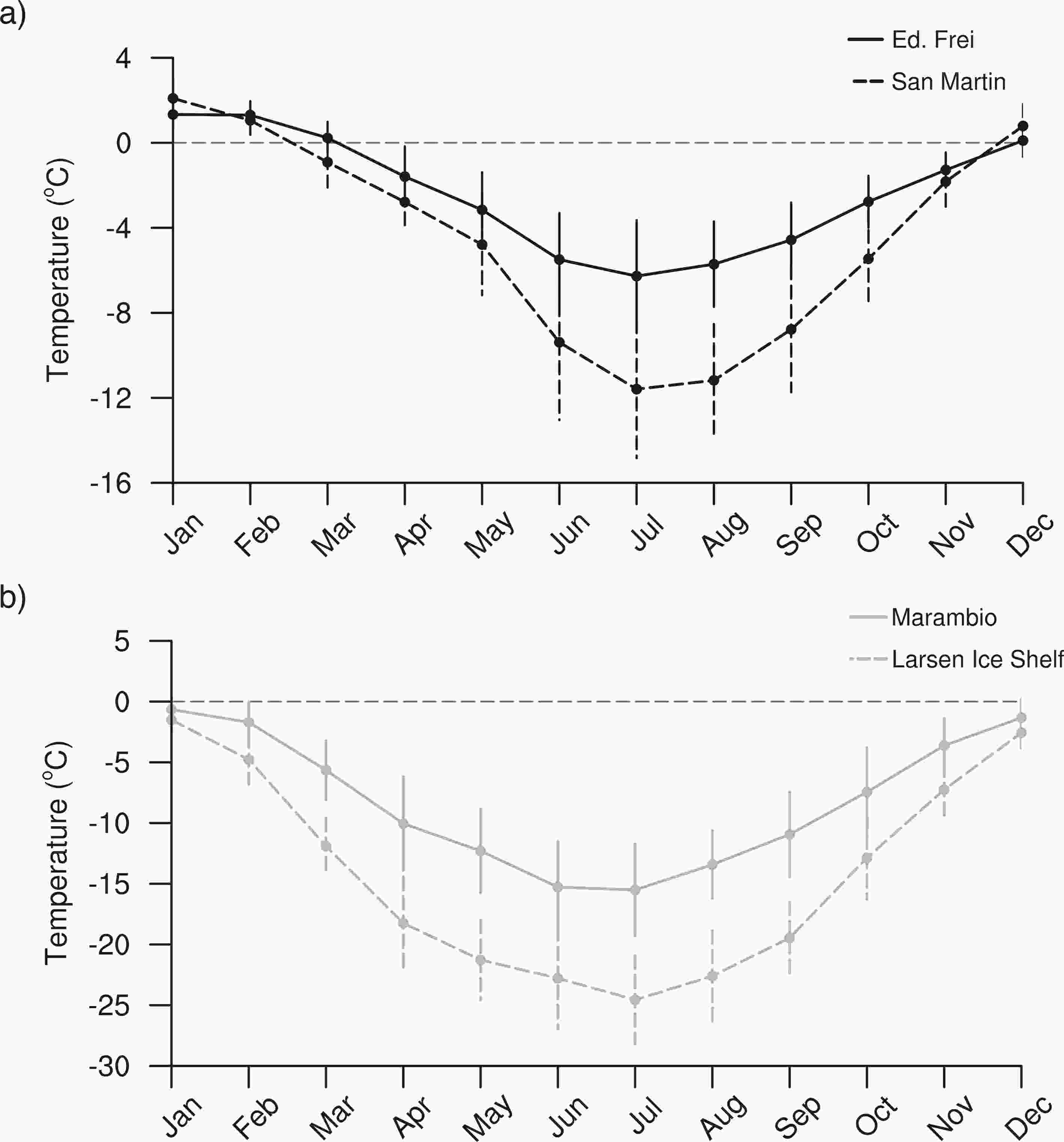 Figure3. The 26-year (1991?2015) mean annual cycle of near-surface air temperature for (a) San Martin (dashed black line) and Frei (solid black line) stations on the windward side, and (b) Larsen Ice Shelf (dashed gray line) and Marambio (solid gray line) stations on the leeward side. Error bars indicate the observed interannual variability of the respective month (ЁР1 sigma).
Figure 4 presents the 1991?2015 time series of summer, autumn and annual mean near-surface temperature for the windward and leeward stations. A trend of summer cooling exists on both sides, except at the San Martin station where this is a trend of +0.02ЁуC (10 yr)?1 (not significant) (Figs. 4a and b). The largest summer cooling trend is observed at the Larsen Ice Shelf station [?0.92ЁуC (10 yr)?1, p < 0.05]. In autumn, a marked statistically significant warming takes place at the San Martin station [+0.64ЁуC (10 yr)?1]. Slight autumn warming occurs at the Frei, Marambio and San Martin stations, whereas the Larsen Ice Shelf station shows a cooling trend [?0.38ЁуC (10 yr)?1]. At the annual scale, trends show a notable cooling at the Larsen Ice Shelf station [?1.1ЁуC (10 yr)?1, p < 0.05]. Although Marambio station shows a non-significant annual trend of ?0.08ЁуC (10 yr)?1, a clearer cooling trend exists and autumn warming is replaced by cooling at Marambio station (not shown) when using the same time period for both Larsen Ice Shelf and Marambio on the leeward side (i.e., 1996?2015), which is consistent with the findings of Jones et al. (2019). On the windward side, located at a latitude close to the Larsen Ice Shelf station, the San Martin station shows a statistically significant warming trend [+0.52ЁуC (10 yr)?1].
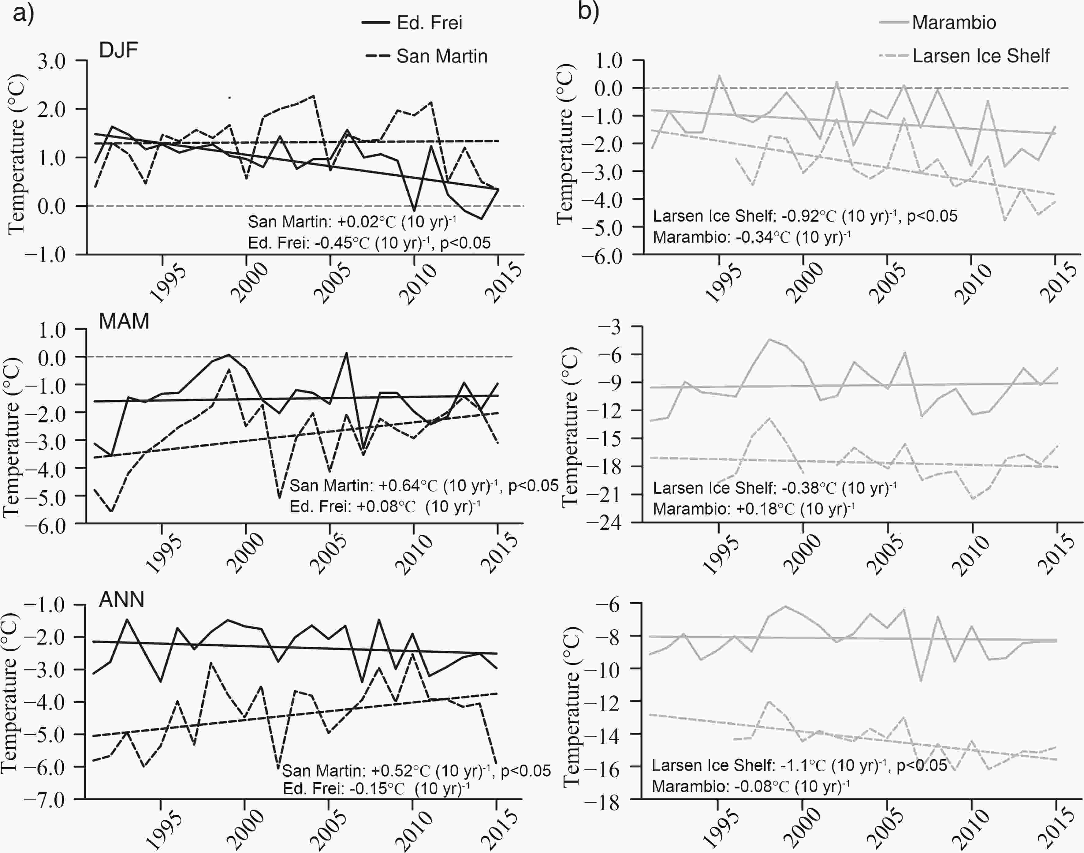 Figure4. Time series (1991?2015) of summer (DJF, top plots), autumn (MAM, middle plots) and annual (bottom plots) near-surface air temperature for (a) San Martin (dashed black line) and Frei (solid black line) stations on the windward side, and (b) Larsen Ice Shelf (dashed gray line) and Marambio (solid gray line) stations on the leeward side. Also included are the trend lines for each plot. Note that when using the same time period for both Larsen Ice Shelf and Marambio on the leeward side (i.e., 1996?2015), a clearer cooling trend exists at Marambio station and autumn warming is replaced by cooling.
2
3.2. Temperature trend in ERA5 and ERA-Interim
Figure 5 compares the near-surface temperature trends [ЁуC (10 yr)?1; 1991?2015] for ERA5 and ERA-Interim on the summer, autumn and annual time scales. In general, both gridded products indicate a cooling trend in summer for almost the entire peninsula [?0.2ЁуC (10 yr)?1 to ?1ЁуC (10 yr)?1], which is more pronounced on the leeward side, in agreement with the observed trends. However, in contrast to ERA5, ERA-Interim shows a warming trend (although not statistically significant) in the central-southern coastal windward side (Alexander Island) (Fig. 5b). Unlike the overall cooling trend in summer, both products show the existence of a clear warming in major parts of the peninsula in the autumn season. Particularly, ERA-Interim exhibits a statistically significant warming on the southern windward coasts and central leeward side (Alexander Island and Larsen Ice Shelf region) [approximately +1.5ЁуC (10 yr)?1]. This pronounced warming depicted by ERA-Interim appears weakened in ERA5, especially over Alexander Island [+0.6ЁуC (10 yr)?1 to +1.0ЁуC (10 yr)?1]. Compared to ERA-Interim, the weaker warming trend in ERA5 exists also over the inland territory of the Antarctic Peninsula, particularly over the northern and central parts. At the annual time scale, the warming on the Larsen Ice Shelf region is notable in both reanalyses [+0.2ЁуC (10 yr)?1 to +0.6ЁуC (10 yr)?1, mostly non-significant]. A general dipole-like trend pattern over the Antarctic Peninsula (i.e., the windward warming and leeward cooling) exists at the annual time scale, except at the Larsen Ice Shelf. This dipole-like trend is largely confined to the coastal zones of both sides.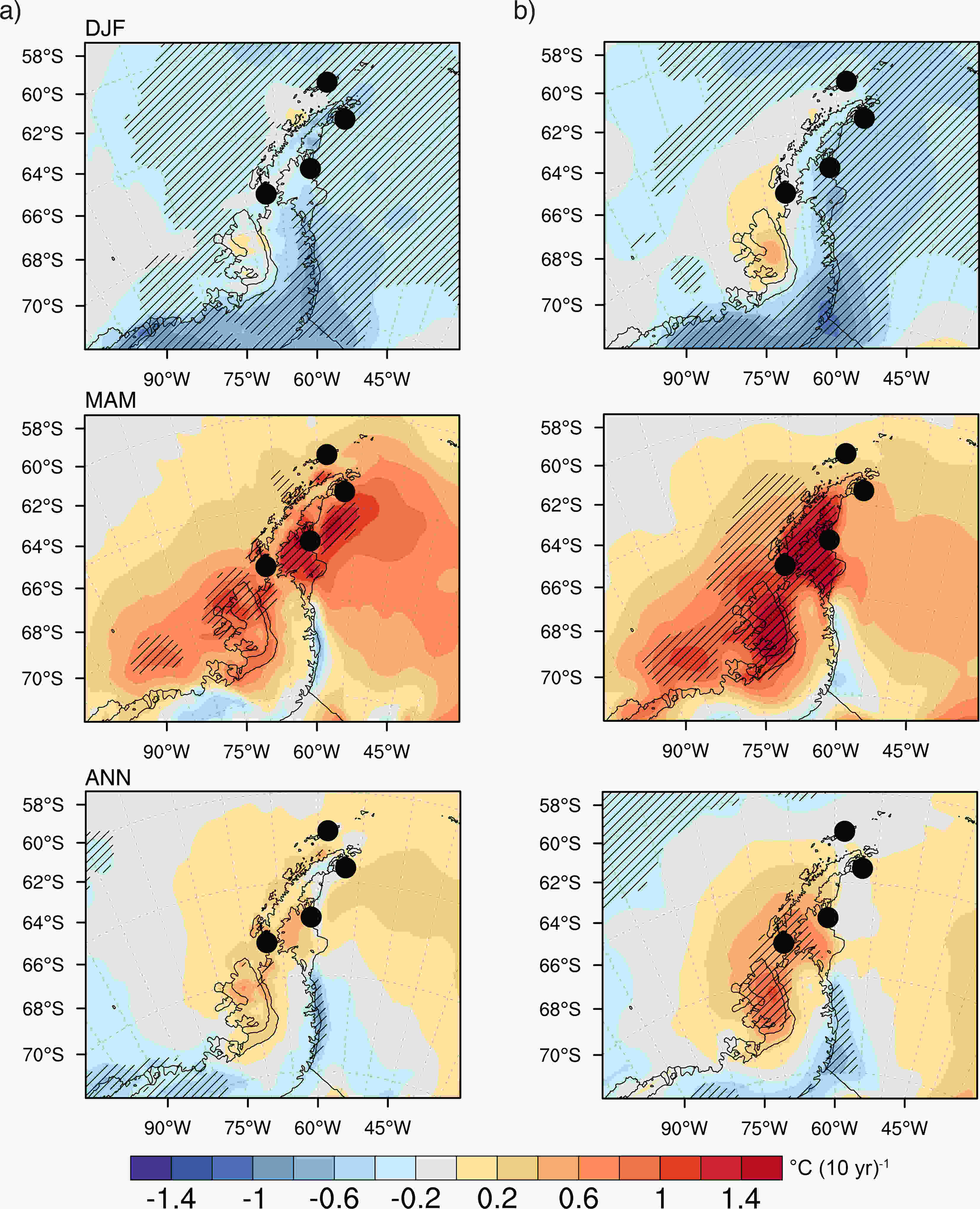 Figure5. Spatial distribution of near-surface temperature trends (1991?2015) for summer (DJF, top plots), autumn (MAM, middle plots) and the whole year (bottom plots) from (a) ERA5 and (b) ERA-Interim. The filled black circles show the locations of meteorological stations used in this study. Regions with statistically significant trends at the 95% confidence level based on a two-tailed StudentЁЏs t-test are hatched.
To illustrate the potential role of atmospheric circulation changes on the temperature trend contrasts of the summer and autumn seasons, we compare the summer and autumn trends (1991?2015) in mean sea level pressure and 850-hPa wind components (u, v) from ERA5 in Fig. 6. In general, the most notable change in the summer season is the strengthening of the Weddell Sea low [?2 hPa (10 yr)?1] and an anticyclonic trend over the Amundsen Sea (Fig. 6a). In autumn, on the contrary, deepening of the ASL [?4 hPa (10 yr)?1] dominates over the West Antarctic sector. In connection with these summer?autumn surface circulation changes, low-level westerlies (850 hPa) tend to be weakened and strengthened over the South Pacific in the summer and autumn seasons, respectively (Fig. 6b). The existence of a dipole-like pattern of sea level pressure trend in the summer season (i.e., windward anticyclonic and leeward cyclonic conditions) is associated with the strengthening of northward (positive) meridional winds over the Antarctic Peninsula, indicating the possibility of more advection of cold air from the continent (Fig. 6c). On the other hand, the strengthening of southward (negative) meridional winds in the autumn season could lead to the transport of warmer midlatitude air to the Antarctic Peninsula, particularly to the windward side. Compared to ERA5, the amplified leeward warming observed in ERA-Interim in the autumn season could be associated with a more strengthened ASL [?5 hPa (10 yr)?1] and southward winds, and thus moister conditions over the Antarctic Peninsula in ERA-Interim [Figs. S1 and S2 in the electronic supplementary material (ESM)].
 Figure6. Spatial distribution of summer (DJF, left plots) and autumn (MAM, right plots) trends in (a) mean sea level pressure, (b) 850-hPa zonal wind and (c) 850-hPa meridional wind, from ERA5 for the period 1991?2015. Regions with statistically significant trends at the 95% confidence level based on a two-tailed StudentЁЏs t-test are hatched.
2
3.3. Comparison of numerical simulations to observations and reanalyses
A comparison of the recent period (1991?2012) near-surface air temperature and sea level pressure climatology from ERA5, ERA-Interim and numerical simulations is provided in the supplementary material (Fig. S3 in the ESM). Overall, simulations generally capture the temperature and sea level pressure climatology; that is, a relatively mild and humid marine climate on the western coast and a colder continental climate on the east coast.To illustrate more details of the spatiotemporal differences between the simulations and reanalysis products, we provide the mean annual cycle of near-surface temperature for the windward and leeward sides in Fig. 7. On the windward side, ERA5 and ERA-Interim are very close to each other, with temperatures above 0ЁуC in the summer months and around ?6ЁуC in the winter months (Fig. 7a). Dynamically downscaled simulations show a significantly colder annual cycle to those in the boundary conditions (ERA-Interim) and ERA5, particularly in winter months (~2ЁуC difference). On the leeward side, ERA5 indicates colder temperatures compared to ERA-Interim, especially from April to September (Fig. 7b). RACMO reproduces almost the same annual cycle as its boundary conditions (ERA-Interim). Both Polar-WRF simulations exhibit a similar annual cycle, but with much lower temperatures in winter months (approximately ?20ЁуC). Some differences in radiative fluxes (i.e., surface downwelling longwave radiation) in Polar-WRF over the leeward side (see Fig. S4 in the ESM) can lead to a more pronounced radiative cooling with either too little cloud or clouds that are optically thin (King et al., 2015; Deb et al., 2016; Listowski et al., 2017). Station-based comparisons indicate that both reanalysis products and numerical simulations generally capture the observed annual cycle at each station (Fig. S5 in the ESM). However, large winter temperature differences between Polar-WRF and RACMO simulations at Marambio station (Fig. S5b in the ESM) could be associated with differences in other simulated surface variables such as wind speed and mean sea level pressure (Fig. S6 in the ESM).
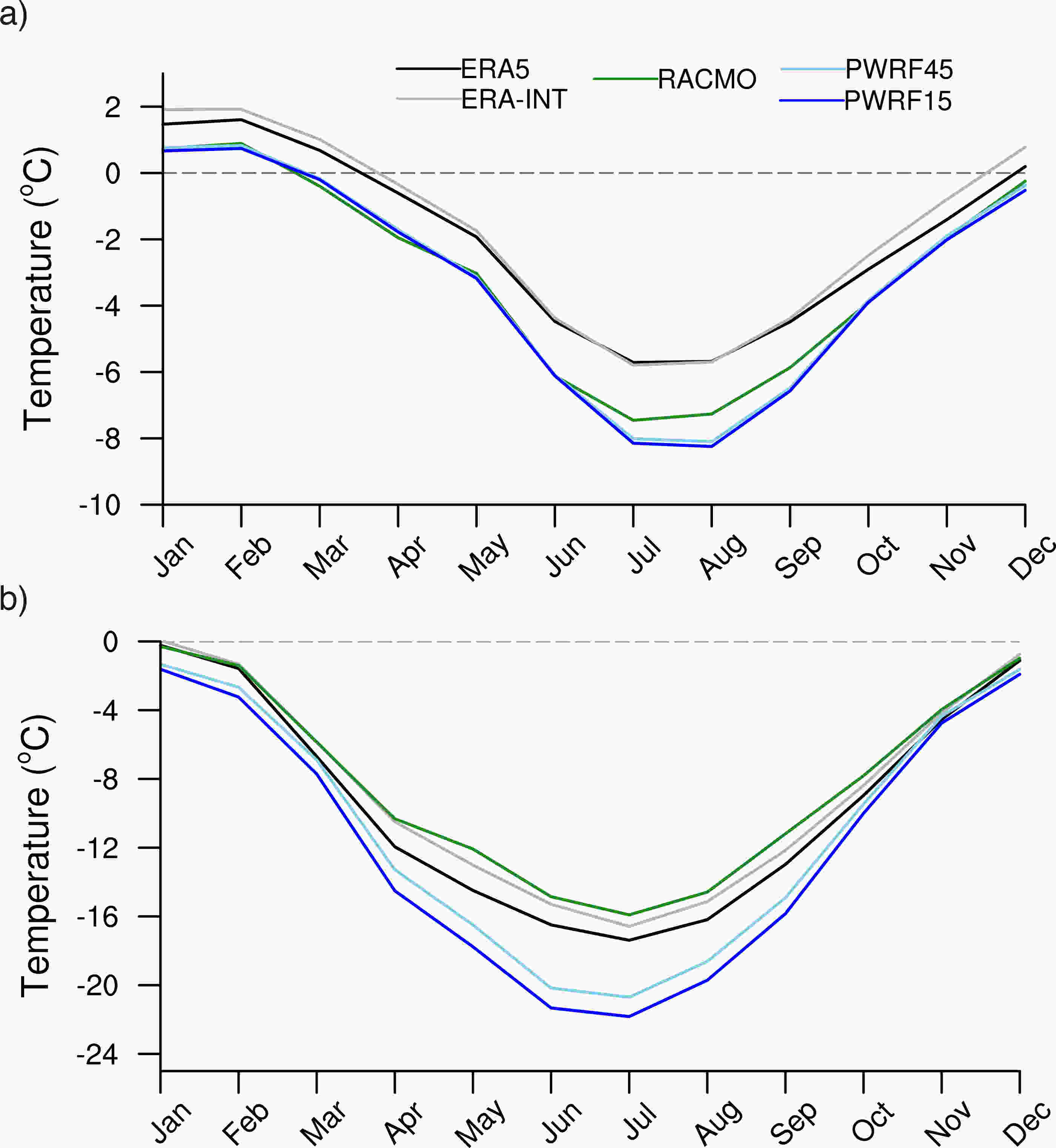 Figure7. The 22-year (1991?2012) mean annual cycle of near-surface air temperature for the (a) windward and (b) leeward side of the Antarctic Peninsula. Black and gray lines correspond to ERA5 and ERA-Interim, respectively. Green, light blue and dark blue lines are the simulations of RACMO, PWRF-45 and PWRF-15, respectively.
Figure 8 compares the maps of summer near-surface air temperature trends (1991?2012) for dynamically downscaled simulations and their boundary conditions (ERA-Interim) as well as ERA5. There is an overall summer cooling over most of the peninsula exhibited by the reanalyses. The warming trend (although not statistically significant) depicted by ERA-Interim (approximately +0.4ЁуC (10 yr)?1, Fig. 8b] over the central-southern windward coasts (Alexander Island) is mostly absent in ERA5 (Fig. 8a), as also illustrated in Fig. 5a. Numerical simulations reproduce the overall cooling trend and, in contrast to the boundary conditions of ERA-Interim, they show a cooling trend over Alexander Island (Figs. 8c-e). It can be speculated that the coarser local details of the topography and land?atmosphere physics in ERA-Interim might account for the existence of different trends. In addition, unlike the RCMs, there is a strengthening of southward (negative) meridional winds at the surface (i.e., 10 m) in ERA-Interim (Fig. S7 in the ESM). Furthermore, westerlies at 10 m tend to be more strengthened in ERA-Interim (p < 0.05), which might prevent cold-air advection from the continent towards the central-southern windward coasts in ERA-Interim. Over the northern tip of the peninsula, both reanalyses and numerical simulations indicate less cooling [approximately ?0.2ЁуC (10 yr)?1] compared to the rest of the peninsula, even with some local warming (non-significant) depicted in the reanalyses and Polar-WRF simulations.
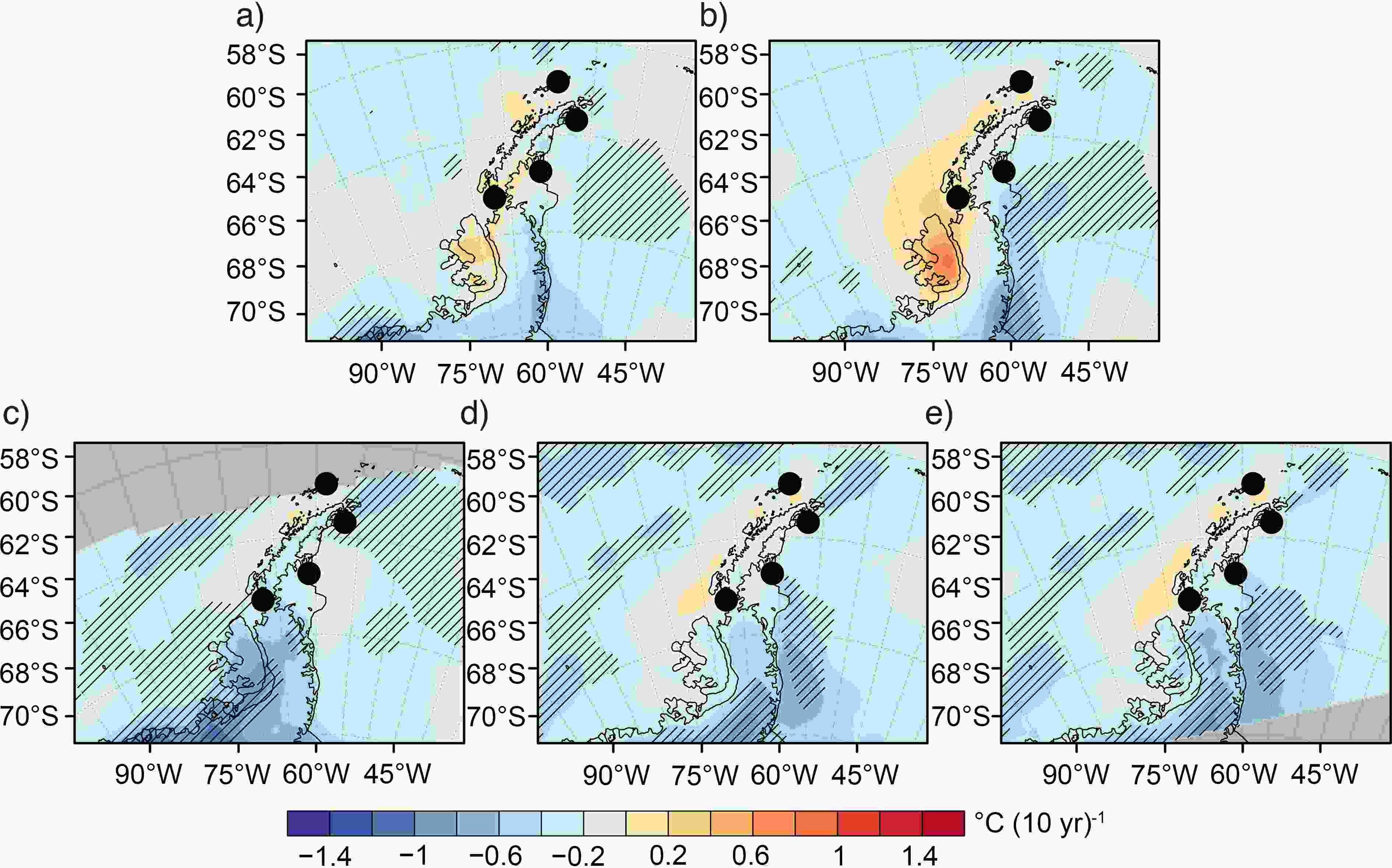 Figure8. Spatial distribution of summer (DJF) near-surface temperature trends (1991?2012) for (a) ERA5, (b) ERA-Interim, (c) RACMO, (d) PWRF-45, and (e) PWRF-15. The filled black circles show the locations of meteorological stations used in this study. Regions with statistically significant trends at the 95% confidence level based on a two-tailed StudentЁЏs t-test are hatched.
The trend map of the autumn season illustrates important differences between the reanalyses and numerical simulations (Fig. 9). Overall, the reanalyses show a warming trend, except on the southern leeward coasts (Figs. 9a and b). On the other hand, the numerical simulations produce a very close trend to each other, exhibiting a marked dipole-like trend pattern over the Antarctic Peninsula (i.e., the windward warming and leeward cooling) (Figs. 9c-e). Unlike the reanalyses, the simulations show a cooling trend over large parts of the leeward side, including the Larsen Ice Shelf region [approximately ?0.2ЁуC (10 yr)?1, non-significant], in agreement with the observed trends. Furthermore, the simulations show a slight cooling trend over some parts of the central-northern peninsula, unlike the boundary conditions. It can be speculated that the impact of the ASL is somehow confined to the windward side in the simulations (Fig. S8 in the ESM); and moreover, unlike the boundary conditions, there is a strengthening of northward (positive) winds at the surface over the central-northern peninsula that might lead to the cooling trend over this region (Fig. S9 in the ESM). Some differences between the simulations also exist on the southeast leeward side, in which Polar-WRF simulations show larger cooling trends (Figs. 9d and e). A comparison of the autumn season time series of surface downwelling longwave radiation over the southeast leeward side shows that Polar-WRF simulations systematically have lower values with negative trends (although not statistically significant) compared to those in RACMO simulations (Fig. S10a in the ESM). Surface variables also illustrate the increasing tendency of drier and colder conditions over the southeast leeward side in Polar-WRF simulations compared to RACMO during the 1991?2012 period (Figs. S10b and c in the ESM).
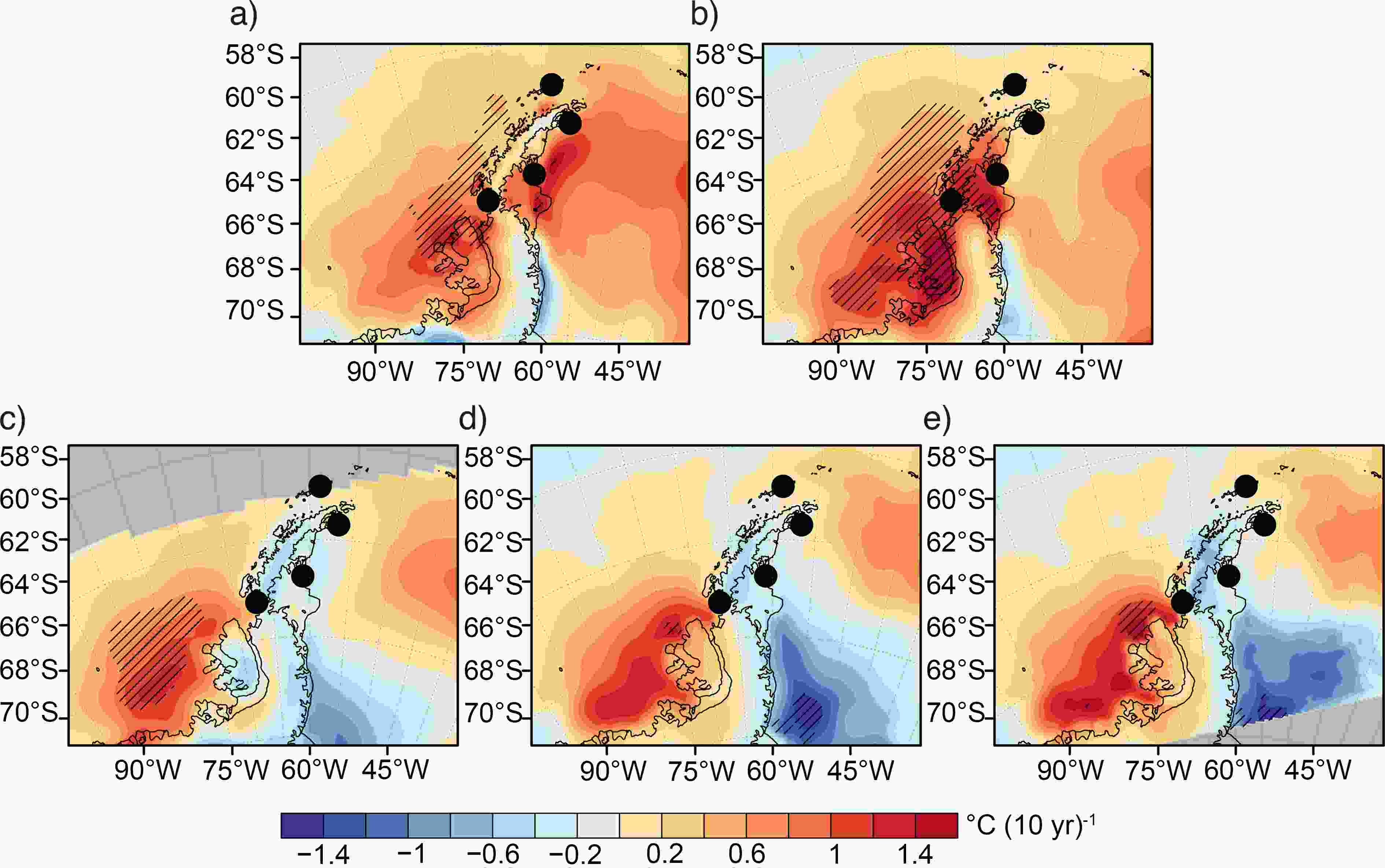 Figure9. Spatial distribution of autumn (MAM) near-surface temperature trends (1991?2012) for (a) ERA5, (b) ERA-Interim, (c) RACMO, (d) PWRF-45, and (e) PWRF-15. The filled black circles show the locations of meteorological stations used in this study. Regions with statistically significant trends at the 95% confidence level based on a two-tailed StudentЁЏs t-test are hatched.
The differences in temperature trends between multiple data sources exist in the annual-scale trend map too. For instance, unlike in ERA-Interim and ERA5, the simulations show a clearer pattern of windward warming and leeward cooling (Figs. 10c-e). On the other hand, although the simulations largely agree on the cooling trend over the central and southern leeward coasts, they differ towards the northern tip of the peninsula, particularly on the eastern side. For instance, unlike in RACMO, Polar-WRF simulations show warming trends over the Larsen A and Larsen B embayments (Figs. 10d and e).
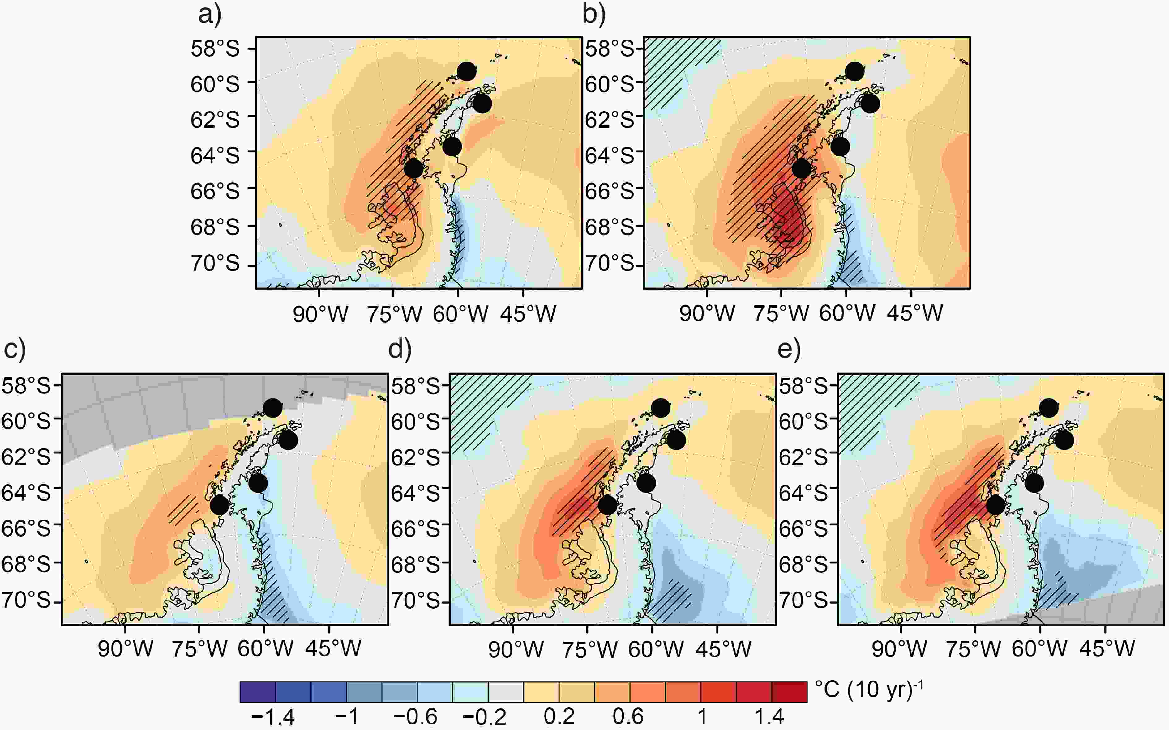 Figure10. Spatial distribution of annual near-surface temperature trends (1991?2012) for (a) ERA5, (b) ERA-Interim, (c) RACMO, (d) PWRF-45, and (e) PWRF-15. The filled black circles show the locations of meteorological stations used in this study. Regions with statistically significant trends at the 95% confidence level based on a two-tailed StudentЁЏs t-test are hatched.
The results presented so far have revealed that there is a notable difference between the reanalyses products and numerical simulations in presenting the recent temperature trends on the central windward and leeward coasts. To delve deeper into this finding, we close this section by comparing the reanalyses and numerical simulations with annual time series of near-surface temperature at the San Martin and Larsen Ice Shelf stations on the central windward and leeward slopes, respectively. San Martin station shows a statistically significant warming trend [+0.9ЁуC (10 yr)?1] for the 1991?2012 period (Fig. 11a). Both reanalysis products exhibit statistically significant warming trends: +0.67ЁуC (10 yr)?1 and +0.83ЁуC (10 yr)?1 for ERA5 and ERA-Interim, respectively. RACMO and PWRF-45 simulations estimate very similar warming trends that are smaller than the observed trend [+0.23ЁуC (10 yr)?1 and +0.27ЁуC (10 yr)?1, respectively]. PWRF-15 gives a statistically significant warming trend of +0.45ЁуC (10 yr)?1. Station-based comparison shows that among the reanalysis products and numerical simulations, PWRF-15 has the largest temporal correlation (r = 0.9) and lowest root-mean-square-difference (1.7ЁуC) for the San Martin station (Table S1). On the leeward side, a marked cooling trend exists for Larsen Ice Shelf station [?1.4ЁуC (10 yr)?1, p < 0.05] for the 1996?2012 period (Fig. 11b). ERA5 shows a smaller cooling trend for the same period [?0.3ЁуC (10 yr)?1], whereas ERA-Interim does not capture the observed annual-scale cooling trend at this station. On the other hand, dynamically downscaled simulations forced with ERA-Interim capture the observed cooling trend at this point, albeit with magnitudes smaller than observed [?0.78ЁуC (10 yr)?1 for RACMO, ?0.74ЁуC (10 yr)?1 for PWRF-45, and ?0.81ЁуC (10 yr)?1 for PWRF-15]. Polar-WRF simulations exhibit the largest temporal correlations (r = 0.83 for PWRF-45 and r = 0.79 for PWRF-15), and PWRF-15 has the lowest root-mean-square-difference (1.9ЁуC) for the Larsen Ice Shelf station comparison (Table S1 in the ESM).
 Figure11. Time series of mean annual near-surface air temperature for the (a) San Martin (1991?2012) and (b) Larsen Ice Shelf (1996?2012) stations. The black solid line denotes the station, while the dashed black and gray lines correspond to ERA5 and ERA-Interim, respectively. The dashed green, light blue and dark blue lines are the simulations of RACMO, PWRF-45 and PWRF-15, respectively.
Observed near-surface temperature trends indicate important contrasts between summer and autumn for the period 1991?2015. A notable summer cooling exists on the northern peninsula (Frei and Marambio stations) and leeward side (Larsen Ice Shelf station). The largest summer cooling trend is observed at the Larsen Ice Shelf station [?0.92ЁуC (10 yr)?1, p < 0.05]. On the other hand, in autumn, San Martin station on the central windward coasts exhibits the largest warming trend [+0.64ЁуC (10 yr)?1, p < 0.05]. Autumn warming is also notable at the other stations except the Larsen Ice Shelf station. At the annual time scale, there is a clear warming trend at San Martin station [+0.52ЁуC (10 yr)?1, p < 0.05], whereas at a close latitude on the leeward side the Larsen Ice Shelf station exhibits a marked statistically significant cooling [?1.1ЁуC (10 yr)?1].
Both ERA5 and ERA-Interim show a summer cooling that is more notable on the central-southern leeward side of the peninsula [?0.64ЁуC (10 yr)?1 to ?1ЁуC (10 yr)?1]. The clear windward warming in autumn depicted by the observations is captured by both reanalyses products. However, important differences in magnitude take place on the central-southern windward coasts. For instance, ERA-Interim shows a remarkable autumn warming over these regions [approximately +1.5ЁуC (10 yr)?1], whereas ERA5 illustrates less warming, especially over Alexander Island [+0.6ЁуC (10 yr)?1 to +1.0ЁуC (10 yr)?1]. A general coastal windward warming and leeward cooling (except the Larsen Ice Shelf) exists at the annual time scale in both reanalyses.
RCM simulations, in general, exhibit good skill in simulating the distinct temperature regimes of the Antarctic Peninsula and reproduce a close spatiotemporal variability to each other. A systematic underestimation of summer and winter temperatures (1ЁуC to 3ЁуC) exists for both PWRF-45 and PWRF-15 over the northern tip of the peninsula. On the other hand, PWRF-15 gives the closest annual cycle shape at the San Martin and Larsen Ice Shelf stations compared to the other simulations and reanalyses. Regarding the temperature trends, unlike the boundary conditions (ERA-Interim) as well as ERA5, Polar-WRF simulations present autumn leeward cooling over the Larsen Ice Shelf region [approximately ?0.2ЁуC (10 yr)?1]. At the annual time scale, both Polar-WRF and RACMO simulations indicate that there is a clear pattern of windward warming and leeward cooling. Unlike in the reanalyses, the numerical simulations exhibit a widespread leeward cooling, including the Larsen Ice Shelf as well as the central-southern parts of the inland territory of the peninsula. Station-based comparisons on the windward side of the central peninsula (San Martin station) show that both reanalyses and numerical simulations agree well with the observed warming trend. On the leeward side of the central peninsula, at the Larsen Ice Shelf station, ERA5 shows a weaker cooling trend than that depicted by the observations, whereas ERA-Interim does not capture the trend. On the other hand, dynamically downscaled simulations forced with ERA-Interim capture the observed cooling trend, indicating the existence of added value.
Despite the long-term warming trend, recent studies also show the existence of a regional cooling trend in some parts of Antarctica, including the Antarctic Peninsula, since the late 1990s (Carrasco, 2013; Turner et al., 2016; Oliva et al., 2017). However, this recent cooling period on the peninsula does not yet represent a shift in the overall robust warming trend, and is instead attributed to internal climate variability (Jones et al., 2016; Gonzalez and Fortuny, 2018; Clem et al., 2019; Jones et al., 2019). The persistent windward warming trend in the autumn season as well as at the annual time scale during the recent cooling period could lead to important implications for the fate of ice sheet surfaces on the windward coasts. Indeed, following the general dipole-like trend pattern over the Antarctic Peninsula (i.e., the windward warming and leeward cooling), the simulations indicate a decreasing and increasing trend in sea ice on the windward and leeward coasts, respectively (not shown). This warming and concurrent ice-sheet surface changes observed on the windward coasts are likely to be associated with the recent deepening of the ASL and anomalous northerly warm advection towards the West Antarctic sector and Antarctic Peninsula depicted by the reanalyses. This large-scale forcing mechanism has also been reported in previous studies (e.g., Bromwich et al., 2013a; Raphael et al., 2016; Jones et al., 2019). Jones et al. (2019) further highlighted the linkage between the recent ASL deepening and a positive Southern Annular Mode trend. On the other hand, the reanalyses show that the summer season is characterized by strengthening of the Weddell Sea low as well as an anticyclonic trend over the Amundsen Sea. This synoptic spatial variability is accompanied by northward (positive) meridional winds, which results in increased transport of cold continental air over the Antarctic Peninsula. This is consistent with the work of Turner et al. (2016), who found that more cyclonic conditions in the northern Weddell Sea are associated with the observed cooling trend over the Antarctic Peninsula. Understanding the determinants of the complex interplay between the strengthening phases of the ASL and Weddell Sea low is an intriguing aspect that deserves further investigation.
As highlighted by Hosking et al. (2013), a correct representation of the ASL is an important factor in representing West Antarctic surface climate characteristics properly in climate models. In a similar manner, compared to ERA5, the amplified autumn leeward warming detected in ERA-Interim could be associated with a more strengthened ASL, and thus moister conditions over the Antarctic Peninsula, which might eventually trigger more episodic leeward Foehn warming (e.g., Cape et al., 2015; Bozkurt et al., 2018; Datta et al., 2019) in ERA-Interim. The better spatial and temporal resolution of ERA5 compared to ERA-Interim tends to reduce the amplified warming trends detected in ERA-Interim over the central-southern windward and leeward sides of the Antarctic Peninsula. This improvement could be associated with better representation of large-scale forcings (e.g., the ASL) as well as the finer local details of the topography and refined land?atmosphere physics. Very recently, some improvements in the performance of ERA5 over ERA-Interim in representing surface climate characteristics of the Antarctic continent were also reported (Tetzner et al., 2019; Gossart et al., 2019).
Finally, regarding numerical simulations, we further demonstrate the potential added value introduced by the dynamically downscaled simulations. For instance, PWRF-15 exhibits higher temporal correlations and lower root-mean-square-differences with respect to the boundary conditions of ERA-Interim for the San Martin and Larsen Ice Shelf stations. Further station-based comparisons with the coarser resolution simulation (i.e., PWRF-45) also indicate that PWRF-15 shows an overall better performance in representing the spatiotemporal variability of the near-surface air temperature, highlighting the importance of the spatial resolution. As illustrated by van Wessem et al. (2015) and Deb et al. (2016), the improved RCM simulations using higher spatial resolution might be crucially important to achieve a better assessment of surface meteorological variables over complex terrain such as the Antarctic Peninsula, particularly along the coastal sites. For instance, Zhang and Zhang (2018) demonstrated that higher resolution simulations are able to resolve foehn warming, and thus tend to produce larger warming and larger temperature fluctuations on the leeward side of the peninsula, including the Larsen Ice Shelf region. In addition to spatial resolution improvement, more research is warranted to further investigate the impact of model tuning and physics schemes on the surface climate characteristics of the Antarctic Peninsula. We have refrained here from comprehensively analyzing the physical mechanisms of some of the local differences in temperature trends depicted by the reanalyses and RCM simulations. Therefore, further research is also needed to better clarify these mechanisms, at both large and local scales, that can lead to large differences of temperature trends in the multiple-data sources.
Acknowledgements. This work was funded by FONDAP-CONICYT (Grant No. 15110009). D. B. acknowledges support from CONICYT-PAI (Grant No. 77190080). This paper is Contribution Number 1588 of the Byrd Polar and Climate Research Center. The authors acknowledge two anonymous reviewers for their constructive comments that helped to improve the manuscript. DB acknowledges the Scientific Committee on Antarctic Research (SCAR) Expert Group on Operation Meteorology in the Antarctic (OPMet) for a partial funding award for the 14th Workshop on Antarctic Meteorology and Climate (WAMC) as well as the Year of Polar Prediction in the Southern Hemisphere (YOPP-SH) meeting in Charleston, SC, USA, between 25 and 28 June 2019. We thank David B. REUSCH (Department of Earth and Environmental Science, New Mexico Technology), Rodrigo Delgado URZЈВA (DirecciЈЎn General de AeronЈЂutica Civil, Chile), Kevin MANNING (National Center for Atmospheric Research, Boulder, Colorado), Andrew ORR (British Antarctic Survey) and Pranab DEB (Indian Institute of Technology) for useful discussions on the Polar-WRF simulations. We are grateful for data from the SCAR-READER dataset and we wish to acknowledge ECMWF for ERA-Interim and ERA5 data. The Polar-WRF simulations were performed within a project entitled ЁАSimulaciones climЈЂticas regionales para el continente AntЈЂrtico y territorio insular ChilenoЁБ funded by the Chilean Ministry of Environment. This research was partially supported by the Basal Grant AFB 170001 and the supercomputing infrastructure of the NLHPC (ECM-02:Powered@NLHPC). The authors appreciate the support of Amazon Web Services (AWS) for the grants PS_R_FY2019_Q1_CR2 & PS_R_FY2019_Q2_CR2, which allowed us to execute the Polar-WRF simulations on the AWS cloud infrastructure. We thank Francisca MU?OZ, Nancy VALDEBENITO and Mirko DEL HOYO at CR2 for post-processing of Polar-WRF simulations.
Electronic supplementary material: Supplementary material is available in the online version of this article at
Open Access This article is distributed under the terms of the Creative Commons Attribution 4.0 International License (http://creativecommons.org/licenses/by/4.0/), which permits unrestricted use, distribution, and reproduction in any medium, provided you give appropriate credit to the original author(s) and the source, provide a link to the Creative Commons license, and indicate if changes were made.
