HTML
--> --> -->Evaluating LSMs is essential in both model development and in region-specific applications. An increasing number of studies have evaluated LSMs in China, a vast region with a huge human population, complex terrain, and wide variations in climate. Some studies have focused on the Tibetan Plateau (Gao et al., 2015), primarily because land surface processes there influence the Asian summer monsoon. Other evaluations have been conducted to study the dry deposition of nitrogen in North China (Ma et al., 2017), the uptake of water by plant roots over northwestern China (Wang et al., 2018), and the effects of soil texture on the water balance over mainland China (Zheng and Yang, 2016). However, few studies have been devoted to understanding the spatiotemporal patterns of soil moisture, runoff, evapotranspiration, and terrestrial water storage (TWS) in all the major river basins of China.
A comprehensive hydrological evaluation of the Noah LSM with multi-parameterization options (Noah-MP) (Niu et al., 2011) in China is worthwhile. The reason for this is fourfold. First, Noah-MP has been used in premier weather, climate and water models, such as the Weather Research and Forecasting model (Barlage et al., 2015) and the US National Water Model (Maidment, 2017). Second, Noah-MP is unique in terms of allowing uncertainty quantification through multi-physics-based ensemble simulations (Zheng et al., 2019), exhibiting strengths and weaknesses of wide-ranging parameterization schemes, and offering insights for model improvements. Third, Noah-MP has been developed and evaluated in data-rich regions such as the USA (Cai et al., 2014; Lin et al., 2018a, b) and it is important to test whether these parameterizations can perform well in relatively data-poor regions. Fourth, Noah-MP has been chosen as a baseline land component for the new generation of high-resolution regional earth system models under development for East Asia [National Key Research and Development Program of China]. All of these arguments warrant a systemic evaluation of Noah-MP in China, which is particularly meaningful given the fact that it is challenging for hydrological modeling due to poor observational data, extensive human activities, and complex climate/terrain.
This study focuses on the hydrological evaluation of the Noah-MP LSM over China based on four major variables: soil moisture, runoff, evapotranspiration, and TWS. Two major physical parameterization schemes (the runoff scheme and the soil moisture factor for stomatal conductance) are chosen to assess their influence on the hydrological simulations. Section 2 describes the model, data, study domain, and methodology. The evaluation is detailed in section 3. Section 4 discusses the results with multi-scheme comparisons, followed by our conclusions in section 5.
2.1. Noah-MP land surface model
Noah-MP (Niu et al., 2011; Yang et al., 2011) was developed from the original Noah LSM with several major improvements. These include a short-term dynamic vegetation scheme (Dickinson et al., 1998), an updated two-stream radiation transfer model (Yang and Friedl, 2003; Niu and Yang, 2004), a simple groundwater model based on the TOPMODEL-based runoff scheme (Niu et al., 2005), a frozen soil scheme (Niu and Yang, 2006), and a multilayer snowpack (Yang and Niu, 2003). Noah-MP provides multiple parameterization options for the key biogeophysical processes, including dynamic vegetation, canopy stomatal resistance, runoff, groundwater, and a soil moisture factor for transpiration. In this study, we use the default options for different parameterizations. As the dynamic vegetation model still requires improvement (Ma et al., 2017), we use version 3.6 of Noah-MP, with the prescribed climatological leaf area index (LAI) (with a seasonal cycle) for different land use and land cover types. Table 1 shows the parameterization options used in this study.| Physical Process | Option |
| Dynamic vegetation | Prescribed leaf area index |
| Canopy stomatal resistance | Ball–Berry |
| Soil moisture factor for stomatal resistance | Noah (SSiB, and CLM) |
| Runoff and groundwater | SIMGM (SIMTOP, Schaake96, and BATS) |
| Surface layer drag coefficient | Monin–Obukhov |
| Supercooled liquid water | Niu–Yang06 |
| Frozen soil permeability | Niu–Yang06 |
| Radiation transfer | Modified two-stream scheme |
| Snow surface albedo | BATS |
| Rainfall and snowfall | Jordan91 |
| Lower boundary of soil temperature | Noah |
| Snow and soil temperature | Semi-implicit |
Table1. Parameterization scheme options used in this study. The tested parameterization schemes in Fig. 10 are shown in brackets.
2
2.2. Study area
The study domain covers the entire area of mainland China (about 9.6 million km2). As China is primarily located in the midlatitudes, the mean annual temperature was 7.68°C and the mean annual precipitation was 719.51 mm during the period 2001–14. The amount of precipitation shows a clear gradient, decreasing from northwest to southeast, whereas the temperature increases from northwest to southeast (shown in Figs. 1c and d). To evaluate the hydrological simulation at both national and basin scales, we divide China into six river basins—namely, the Yangtze, Yellow, Huaihe, Haihe, Pearl, and Songliao River basins (shown in Fig. 1a). Table 2 shows the climatic conditions for the six river basins.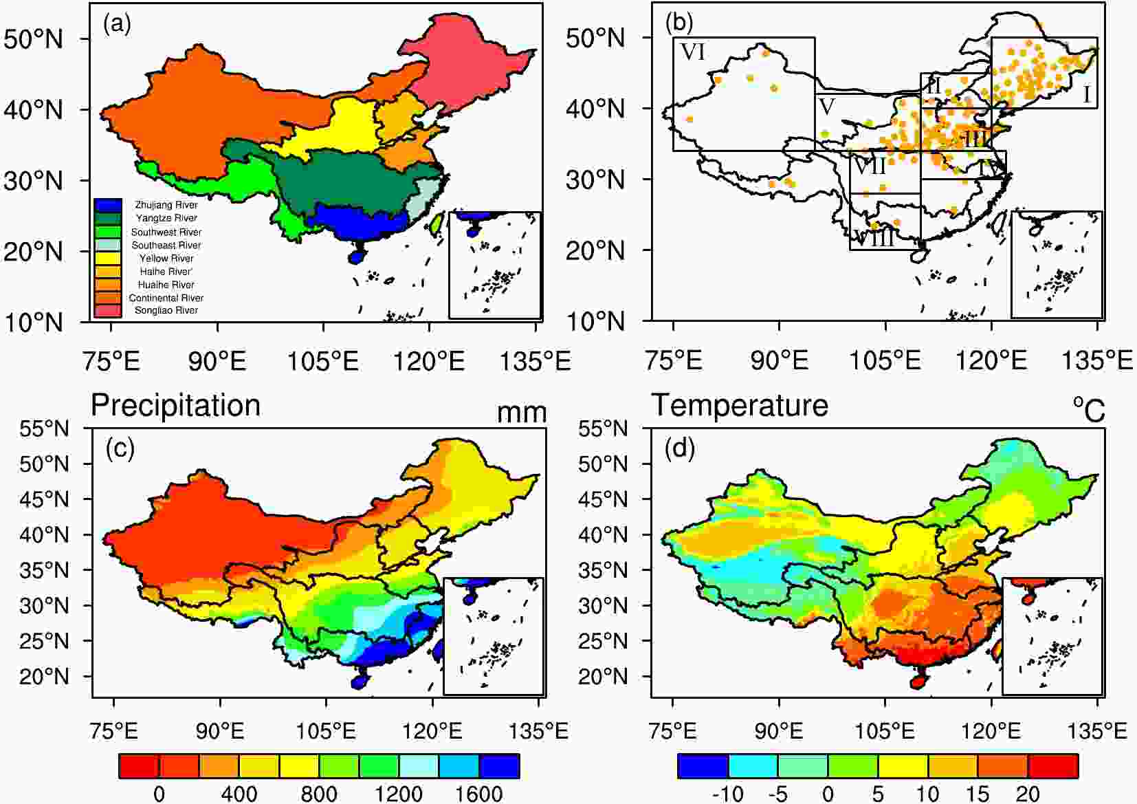 Figure1. Map of China showing (a) river basins, (b) the eight regions defined in Table 3, and average annual (2001–14) (c) precipitation and (d) temperature. The dots shown in (b) represent the distribution of soil moisture stations.
| Region | Area (km2) | Rainfall (mm yr?1) | Temperature (°C) |
| China | 9.63 × 10⁶ | 759 | 7.85 |
| Yangtze River | 1.80 × 10⁶ | 932 | 9.26 |
| Yellow River | 8.09 × 10⁵ | 443 | 5.66 |
| Huaihe River | 3.24 × 10⁵ | 895 | 14.23 |
| Haihe River | 3.17 × 10⁵ | 517 | 9.38 |
| Pearl River | 5.35 × 10⁶ | 1534 | 19.17 |
| Songliao River | 1.24 × 10⁶ | 550 | 3.09 |
Table2. Size and climatic conditions in the study area and its subregions.
2
2.3. Input data
32.3.1. Model input data
For atmospheric forcing, we use version 2 of the Global Land Data Assimilation System (GLDAS) reanalysis dataset (Rodell et al., 2004), which integrates a huge quantity of observation-based data. The version 2.0 meteorological forcing data from GLDAS, at a spatial resolution of 0.25° × 0.25° and three-hourly temporal resolution, are entirely based on Princeton meteorological forcing data, whereas the version 2.1 data combine model, remote sensing, and observation-based forcing datasets. Our initial comparisons of the Noah-MP simulation results using these two versions of forcing data (not shown) suggest that version 2.1 produces a better simulation of soil moisture, evapotranspiration, and TWS in most of China, with higher correlation coefficients and lower root-mean-square errors (RMSEs) during the period 2000–10. However, only version 2.0 provides forcing data before 2000, a period when our runoff observations are available. Thus, to reconcile the model performance and data availability issues, we combine both versions of the forcing data such that version 2.0 of GLDAS is used as the forcing data from 1959 to 1999, and version 2.1 as the forcing data from 2000 to 2014.GLDAS also provides static input data for this study, including land use and land cover types (Friedl et al., 2010), a land water mask (Carroll et al., 2009), soil texture (Reynolds et al., 2000), and elevation (GTOPO30). The prescribed LAI data come from the MODIS dataset, with the climatological data varying by month.
3
2.3.2. Observational data for soil moisture
We obtain the observed soil moisture data from the Chinese Crop Growth and Farmland Soil Moisture Dataset of the China Meteorological Administration’s Science Data-sharing Network (To best match the simulation results considering the availability of observational data, we only compare the soil moisture at a depth of 10 cm, after converting its units from relative humidity to volumetric content. These sites are mainly distributed in eastern China (Fig. 1d). Although the spatial and temporal distribution appears relatively sparse, this soil moisture dataset covers the most extensive area in China over the longest time period. Part of this dataset has also been integrated into the Global Soil Moisture Database by Robock et al. (2000), so it is a reliable observational dataset for evaluating LSMs.
To ensure comparability and avoid the continuity problem caused by missing values, we choose 2001–13 as the analysis period and divide it into spring, summer, and autumn for further analysis. After data quality control, which means only using those sites whose missing values account for less than 15% of the whole period, the number of qualified stations is 134 for spring (March–April–May, MAM), 130 for summer (June–July–August, JJA), and 118 for autumn (September–October–November, SON). These stations are grouped into eight regions (shown in Fig. 1b) based on the spatial patterns of the dryness and wetness centers throughout the domain, as defined in Table 3 (Liu and Xie, 2013).
| Identification | Name | Longitude | Latitude |
| I | Northeast | 120°–135°E | 40°–50°N |
| II | Northern North | 110°–120°E | 40°–45°N |
| III | Southern North | 110°–120°E | 34°–40°N |
| IV | Middle and Lower Yangtze River basin | 110°–125°E | 30°–34°N |
| V | Eastern Northwest | 95°–110°E | 34°–42°N |
| VI | Western Northwest | 80°–95°E | 34°–50°N |
| VII | Northern Southwest | 100°–110°E | 28°–34°N |
| VIII | Southern Southwest | 100°–110°E | 20°–28°N |
Table3. Location of eight subregions for soil moisture division.
3
2.3.3. Observational data for runoff
Monthly streamflow data are from Dai et al. (2009), which are derived from natural discharge considering losses due to human activities in the upper reaches. Datong, Wuzhou, Bengbu, Gaocung, and Chilling stations are chosen, representing the Yangtze, Xijiang, Huaihe, Yellow, and Liaohe River basins, respectively. Among these sites, the Yangtze, Yellow, and Liaohe stations provide monthly data from 1960 to 1999, whereas Huaihe provides data from 1960 to 1989 and Xijiang from 1960 to 1986. To compare the runoff pattern for the whole domain, we use the University of New Hampshire Global Runoff Data Center (UNH-GRDC) dataset as a source of monthly gridded climatological runoff composite fields, which combines the measured discharge with the output from a hydrological balance model (Fekete et al., 2002). In addition, the MERRA-Land (Reichle et al., 2011) and GLDAS-Noah (Rodell et al., 2004) climatology runoff datasets are also used because of potential uncertainty/errors contained in a single reference dataset.3
2.3.4. Observational data for evapotranspiration
FLUXNET-MTE (model tree ensemble) is chosen to evaluate the evapotranspiration simulation. Jung et al. (2009) combined FLUXNET observations at 253 sites with satellite data and land surface meteorological data and used the MTE algorithm to produce gridded FLUXNET-MTE data at 0.5° and monthly resolution covering the period 1982–2011. This dataset has been used to detect and attribute the decrease in global land evapotranspiration (Jung et al., 2010), improve version 4 of the Community Land Model with enhanced canopy processes (Bonan et al., 2011), and reveal the spatiotemporal patterns of evapotranspiration in response to multiple environmental factors (Shi et al., 2013). In this study, we choose the data from 2001 to 2011 as the validation data.3
2.3.5. Observational data for TWS
The Gravity Recovery and Climate Experiment (GRACE) satellites (Wahr et al., 2004) provide global monthly TWS anomaly data at a resolution of 1°. The data used in this study were derived by Landerer and Swenson (2012) based on Release-05 of the GRACE Level-2 data from the University of Texas at the Austin Center for Space Research. The data from 2003 to 2014 are selected for model evaluation.2
2.4. Spin-up
To reach equilibrium for the model variables (such as water table depth) with longer memories, we use a two-stage procedure for spin-up. First, the atmospheric forcing for the whole year of 1959 from GLDASv2.0 is repeated 70 times, followed by 41 years of integration to cover the period 1960–2000. Second, atmospheric forcing for the whole year of 2000 from GLDASv2.1 is repeated 70 times, followed by 14 years of integration to cover the period 2001–14. The 70-year spin-up has been shown to be sufficiently long to reach equilibrium (Cai et al., 2014). The results for these periods are calculated and evaluated.2
2.5. Simulation performance metrics
The model performance is evaluated using three metrics: the correlation coefficient (R), the RMSE and the Nash–Sutcliffe efficiency (NSE) coefficient (Nash and Sutcliffe, 1970). These three metrics are defined aswhere N is the sample size, Mi is the simulation value, Oi is the observation value,


3.1. Soil moisture
The soil moisture site data can be used to represent the temporal variation in soil moisture over a 500-km radius around each site (Entin et al., 2000). Therefore it is reasonable to compare the site data with the gridded values. We also compare the mean value of all the sites located in each region and their corresponding grids to analyze the consistency, which could reduce the deviation caused by spatially representative differences in the site observations. Here, considering the availability and distribution of the observations, we choose the first five regions for regional comparison. Moreover, the correlation coefficient and RMSE for each site are also presented.Because of the lack of observational data during winter when the soil is frozen, we only compare the spatial distributions of the simulated and observed soil moisture in spring, summer, and autumn (Fig. 2). The observational data show that, in spring, the Yangtze and Huaihe River basins and eastern and northeastern China are humid, while the dry regions are located in northern-central China, consistent with previously reported work (Lai et al., 2016). The simulation captures this pattern and reflects the increase in soil moisture from west to east in northeastern China. Overall, the simulation captures the spatial distribution of soil moisture, but shows wetter conditions in almost the whole domain, especially in eastern China. The simulation also underestimates two sites in northwestern China. These two stations are located near a lake and receive water from snowmelt in spring, which results in their relatively high soil moisture. This discrepancy shows that there is still room for the model to include the influence of both the environment and terrain.
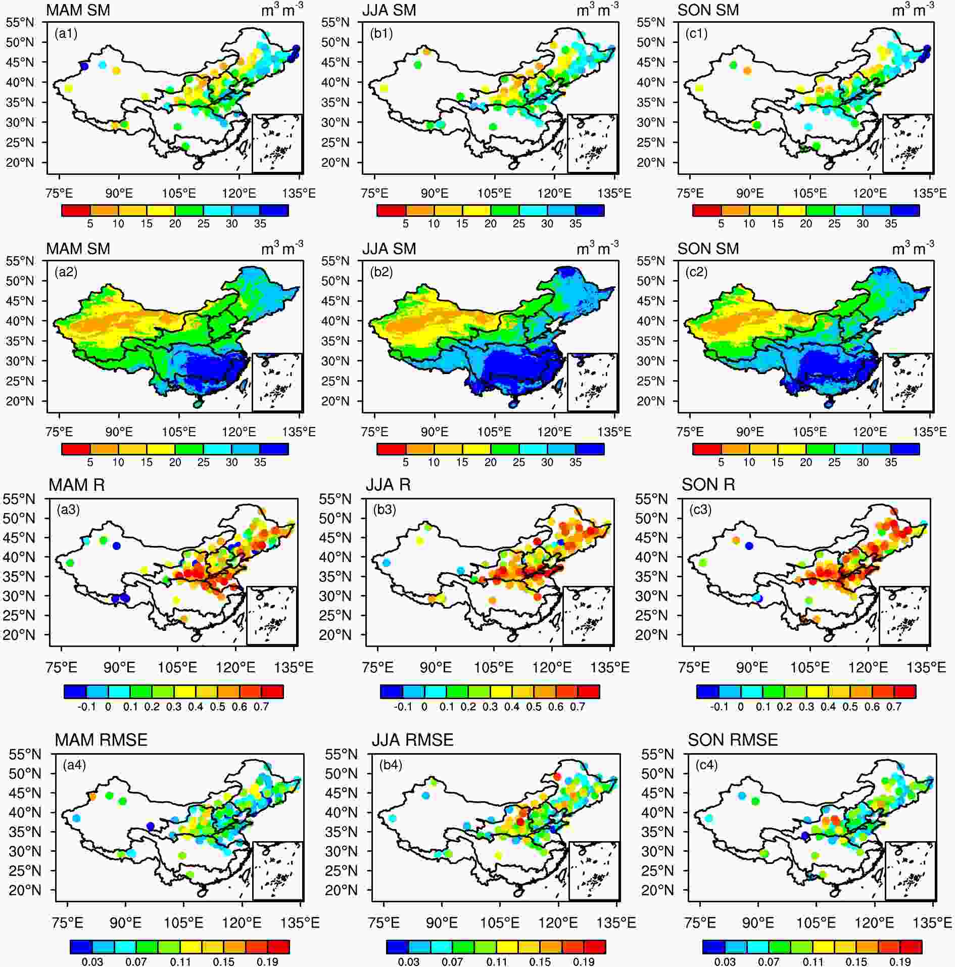 Figure2. Spatial comparison of top 10-cm soil moisture for the 2001–13 period: (a1, b1, c1) mean observations for MAM, JJA and SON, respectively; (a2, b2, c2) same as the first row, but for simulations; (a3, b3, c3) correlation coefficients; (a4, b4, c4) RMSEs. The winter months are excluded due to the issue of frozen soil.
This overall good performance in spring is also applicable to summer and autumn. Both the simulations and observations reflect the contrasting distribution of dry and wet regions in northeastern China, showing wet areas in the central plains and dry areas in the eastern and western mountainous regions. Although we have only four sites in northwestern China, the simulation is also reasonable here. A decreasing trend from east to west in Inner Mongolia and two clear dry centers in western Inner Mongolia and the Tarim basin of Xinjiang are also seen in the simulations. The simulations are better in northeastern China. Although the distribution pattern is captured by the simulations, it is too big in most regions. Both the simulations and observations show slight increases of soil moisture in the middle Yellow River basin and near the junction between the Yellow and Yangtze River basins in SON, when compared with that in JJA. The simulations also capture the observed soil moisture reduction in the northeastern Yangtze River basin. However, the simulations fail to reproduce the increase at some sites in the Yangtze River basin. In SON, precipitation is less than in JJA, which reduces soil moisture. The SON temperature is also smaller than in JJA, contributing to the soil moisture increase. They both affect the soil moisture at the same time, resulting in different variation trends. As such, the model is unable to reproduce the SON soil moisture, leaving room for further development.
Figure 2 shows that the simulations are better in summer and autumn than in spring because it is challenging to reproduce the soil moisture during spring in the presence of snow and ice melt. Overall, as shown in Table 4, the sites located in the northeast (region I), southern North China (region III), and the middle and lower Yangtze River basin (region IV) show a relatively high correlation. Most stations show reasonable results for the RMSE, except for several sites in the Yellow River region—the region with complex terrain and dense population. The simulation therefore captures the spatial distribution of soil moisture, but overestimates the soil moisture in all three seasons. This overestimation could be a result of uncertainty in forcing data. We compare our precipitation forcing datasets with the gridded monthly data provided by the China Meteorological Administration based on site-observed values (shown in the Electronic Supplementary Material, Fig. S1), and find that our forcing is larger in most regions in northeastern and southern North China where most sites are located in MAM, JJA, and Son. Although this overestimation is marginal, it still might explain the overestimation in soil moisture in these regions to some extent. Human activities such as irrigation, groundwater withdrawal, and reservoirs and dams also influence the soil moisture, but the sign and magnitude of the influence depend on the type of human activities, which is region-specific. In this study, Noah-MP does not include any of these activities. The sparseness of in-situ soil moisture data and coarse resolution in the simulations makes it difficult to pinpoint the exact causes of modeling deficiencies.
| Identification | RMSE (m3 m?3) | R | No. of sites | |
| MAM | I | 7.15×10⁻⁴ | 0.733 | 40 |
| II | 7.78×10⁻⁴ | 0.760 | 10 | |
| III | 5.97×10⁻⁴ | 0.347 | 40 | |
| IV | 1.10×10⁻³ | 0.262 | 8 | |
| V | 5.56×10⁻⁴ | 0.346 | 19 | |
| JJA | I | 5.76×10⁻⁴ | 0.898 | 40 |
| II | 6.83×10⁻⁴ | 0.734 | 10 | |
| III | 5.24×10⁻⁴ | 0.906 | 37 | |
| IV | 7.73×10⁻⁴ | 0.539 | 7 | |
| V | 4.89×10⁻⁴ | 0.723 | 18 | |
| SON | I | 6.75×10⁻⁴ | 0.948 | 34 |
| II | 9.81×10⁻⁴ | 0.707 | 5 | |
| III | 8.55×10⁻⁴ | 0.886 | 39 | |
| IV | 8.35×10⁻⁴ | 0.406 | 7 | |
| V | 6.77×10⁻⁴ | 0.823 | 16 |
Table4. Correlation coefficient (R) and root-mean-square-error (RMSE) between the simulated and measured detrended soil moisture and the number of sites in different regions from 2001 to 2013. Winter is excluded due to the issue of frozen soil.
Considering the differences in spatial representativeness between the site observations and gridded simulations, we use regionally averaged detrended values for comparison. Based on the spatial distribution of the stations, we compare five basins (Table 3). All of the correlation coefficients are relatively high, especially for the northeastern and northern north regions (regions I and II), which have the most sites for the three seasons and show the highest correlation between the observations and simulations. All the values pass the 95% confidence test, suggesting that the simulation can reproduce the interannual variability well. The RMSE of the eastern northwest region (region V) is better than that for the other regions. Note that the middle and lower Yangtze River basin region (region IV) simulation requires improvement, which may be due to the small number of soil moisture measurement sites.
2
3.2. Runoff
Because runoff has impacts on water resources management and the subsequent redistribution of environmental and economic benefits, it is important for LSMs to be able to reproduce and predict runoff.Figure 3 shows that the Noah-MP simulations capture the spatial distribution of runoff relative to the UNH-GRDC, MERRA and GLDAS_Noah datasets. The pattern of runoff is similar to that of precipitation, with a gradual increase from northwestern to southeastern China. However, the simulation does not reproduce the data from some small regions in southern China. The simulation gives the highest value in southwestern China of these four datasets, with the multi-year mean annual value (265 mm) closest to that in the GRDC dataset (271 mm).
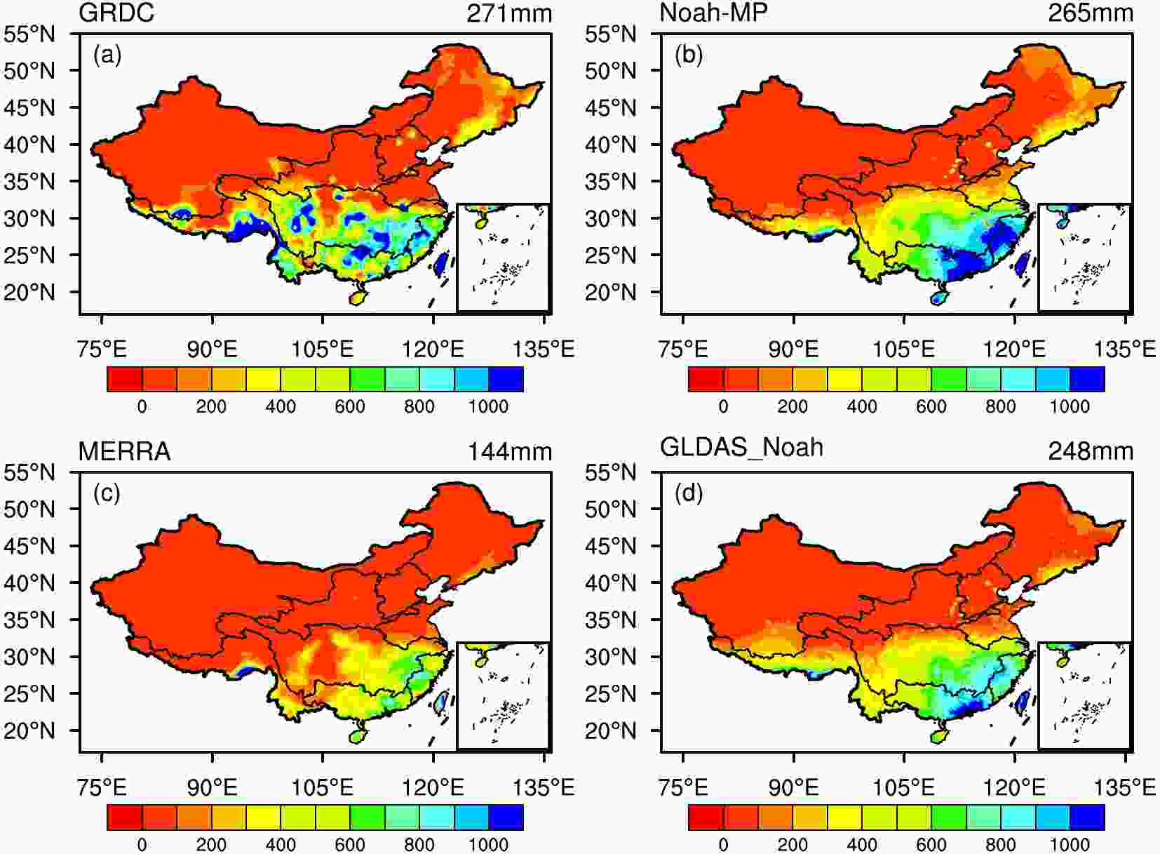 Figure3. Spatial distribution of (a) GRDC, (b) Noah-MP simulated, (c) MERRA, and (d) GLDAS_NOAH climatological annual-mean runoff. The numbers in the top-right of each figure are the annual-average runoff (mm).
Figure 4 shows the distribution of five hydrological stations and their river systems. There is considerable consistency between the observed and simulated annual mean anomalous runoff over these basins, with the correlation coefficients generally greater than 0.8. The NSE is also satisfactory. Specifically, the Yangtze River ranks the best for the NSE (0.8) and also has the largest correlation coefficient (0.91) among these five basins, followed by the Huaihe and Xijiang Rivers, which shows the ability of the model to simulate streamflow in semi-humid and humid areas. By contrast, the Yellow River has a relatively low NSE due to its complex terrain and high levels of human activity, such as irrigation and the construction of dams. The Liaohe River has the smallest correlation coefficient because it is located mostly in a semiarid region, where many LSMs still struggle to reproduce the streamflow patterns and dynamics (Xia et al., 2012).
 Figure4. Location of stations and comparison of simulated and observed runoff anomalies in 1960–2000, where R is the correlation coefficient, NSE is the Nash–Sutcliff efficiency, and the regression lines are shown for these five sites.
Figure 4 also shows that the Noah-MP LSM reproduces the variation trend of the four basins well, except for the Liaohe River. Specifically, the simulation captures the significant decreasing trend of the Yellow River and the increasing trend of the Yangtze and Xijiang Rivers, which is consistent with previously published research (Li et al., 2017). The simulation also captures the peak and lowest values of the observational dataset in most regions. From the viewpoint of the interdecadal variation, the simulation reproduces the switch from an increasing trend to a decreasing trend during the 1980s to 1990s in the Liaohe River basin and the change from an increasing to a decreasing trend in the Huaihe River basin during the 1960s to 1970s.
In addition to the forcing and static data, errors in the runoff simulation can also be caused by a number of other factors. First, the observational data are obtained directly at fixed times and locations, but do not record where the water comes from and the relevant pathways. Therefore, the data cannot distinguish between precipitation and irrigation, resulting in considerable uncertainties. Second, the model does not include human activities, such as the tile drainage process, which is an important agricultural method used to adjust the soil moisture content and subsequently influences the amount of runoff and groundwater. In addition, some parameters are initially defined by the modelers using locally calibrated values, making it difficult for the simulations to match the observations in all the basins when using the same set of parameters, causing greater uncertainties and larger errors.
2
3.3. Evapotranspiration
As the sum of water transport from the land surface to the atmosphere, evapotranspiration has significant effects on the water, energy, and carbon cycles through land–atmosphere interactions (Sellers et al., 1997). The ability of an LSM to simulate evapotranspiration is therefore an important indicator in the evaluation of models.The MTE_Obs dataset shows a strong spatial variation and a clear gradient from the northwest to southeast (Fig. 5). In general, southern China has relatively high evapotranspiration, with the mean annual precipitation (temperature) exceeding 700 mm (10°C) because the temperature and humidity of subtropical basins are sufficient for evapotranspiration. However, these two factors limit evapotranspiration in cold and dry basins and the lowest rates of evapotranspiration are found in the arid and semiarid regions of northwestern China. The simulation captures this spatial pattern well, although there is still a clear difference between the simulation and the MTE_Obs data (Fig. 5c). This underestimation is seen in most regions and especially in southeastern China, although it is not observed in Tibet, Inner Mongolia, and Ningxia Province, consistent with previously reported results (Liu et al., 2016). We also compare the values for skin temperature, which is used in the simulation and in the MODIS data (shown in the supplementary material, Fig. S2); and find the simulation result is smaller in most regions for all the reasons, which contributes to the smaller value of evapotranspiration in the simulation.
 Figure5. Spatial distribution of annual evapotranspiration during the period 2001–11: (a) MTE-derived observation; (b) Noah-MP simulation; (c) Noah-MP minus observation. The white area in northwestern China indicates missing observations.
Through a further comparison of the interseasonal variation, we find that both the MTE_Obs data and the simulation show a clear seasonal variation (shown in the supplementary material, Fig. S3 and Fig. S4) and that the spatial variability is controlled by climatic conditions. Evapotranspiration is at a maximum in summer, whereas the lowest evapotranspiration occurs in winter, showing the limit imposed by the temperature and humidity. The MTE_Obs data decrease from southeast to northwest in all four seasons and the simulation reproduces this pattern, as well as the seasonal dynamics of evapotranspiration, although it still underestimates evapotranspiration in most regions.
To further evaluate the simulation of evapotranspiration, we compare the annual variation in the regional mean anomalies over the six major river basins and the whole of China (Fig. 6). The observed data and the simulation both show a clear interannual variability, with the trend in evapotranspiration being upward during 2001–11. This is in agreement with the reported increase in precipitation in recent years (Ma et al., 2015). The simulation shows a high consistency with the MTE_Obs data in all the regions. Table 5 shows that all the correlation coefficients are greater than 0.7, especially in the Yellow River basin (0.97), which has the smallest RMSE (0.71) and the second largest NSE (0.90). Apart from the Songliao River basin, all the other basins and the simulation for the whole of mainland China show a reasonable NSE, which confirms that the simulation in anomalies is reliable. The simulation reproduces the variation trend on both the national and basin scales, although the mean evapotranspiration is underestimated in most regions.
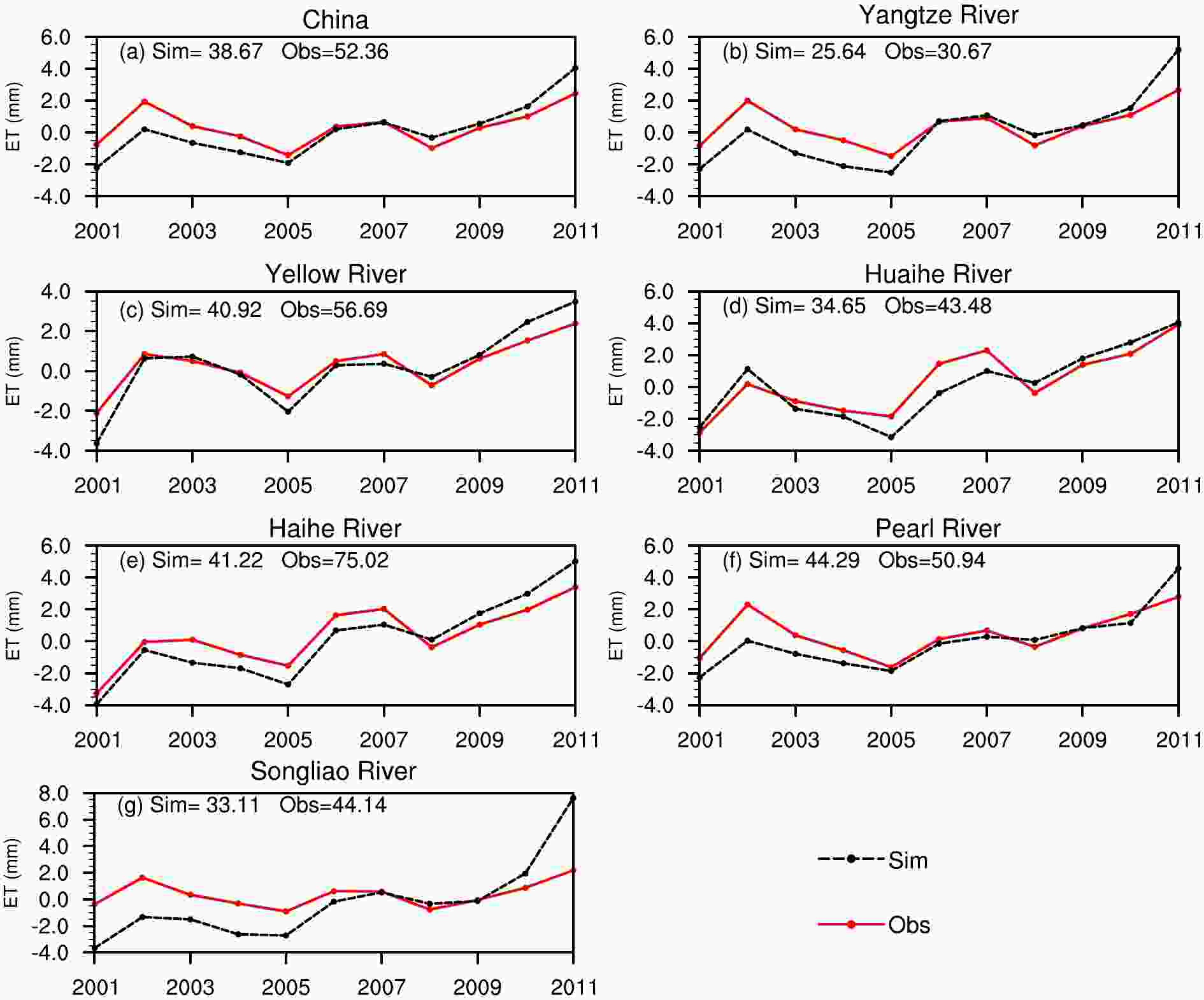 Figure6. Comparison of the evapotranspiration (ET) mean annual anomalies between the results of the simulation and the MTE_Obs data for China and the six major river basins. The numbers given are the mean annual evapotranspiration values.
| Region | R | RMSE (mm) | NSE |
| China | 0.83 | 0.99 | 0.85 |
| Yangtze River | 0.85 | 1.29 | 0.53 |
| Yellow River | 0.97 | 0.71 | 0.90 |
| Huaihe River | 0.91 | 0.92 | 0.93 |
| Haihe River | 0.94 | 1.00 | 0.82 |
| Pearl River | 0.83 | 1.07 | 0.77 |
| Songliao Riverriver | 0.73 | 2.40 | ?1.39 |
Table5. Correlation coefficient (R), root-mean-square-error (RMSE), and Nash–Sutcliffe coefficient (NSE) for the annual evapotranspiration anomalies between the simulation and the FLUXNET-MTE data in different river basins from 2001 to 2011.
2
3.4. Terrestrial water storage
As an important part of the water cycle, TWS plays a significant part in the climate system. The ability to reproduce the TWS reflects the capacity of the LSM in a hydrological simulation. The Noah-MP LSM calculates TWS anomalies using the formulawhere SWEA is the snow water equivalent anomalies, SMCA is the total soil moisture anomalies, and WTDA is the anomalies of water table depth. Their units are mm.
The simulation is consistent with the observations at the national scale (Fig. 7a). Specifically, they both reflect the relatively high level of TWS during 2003?06 and the low level of TWS during 2006?12, when there were frequent droughts (
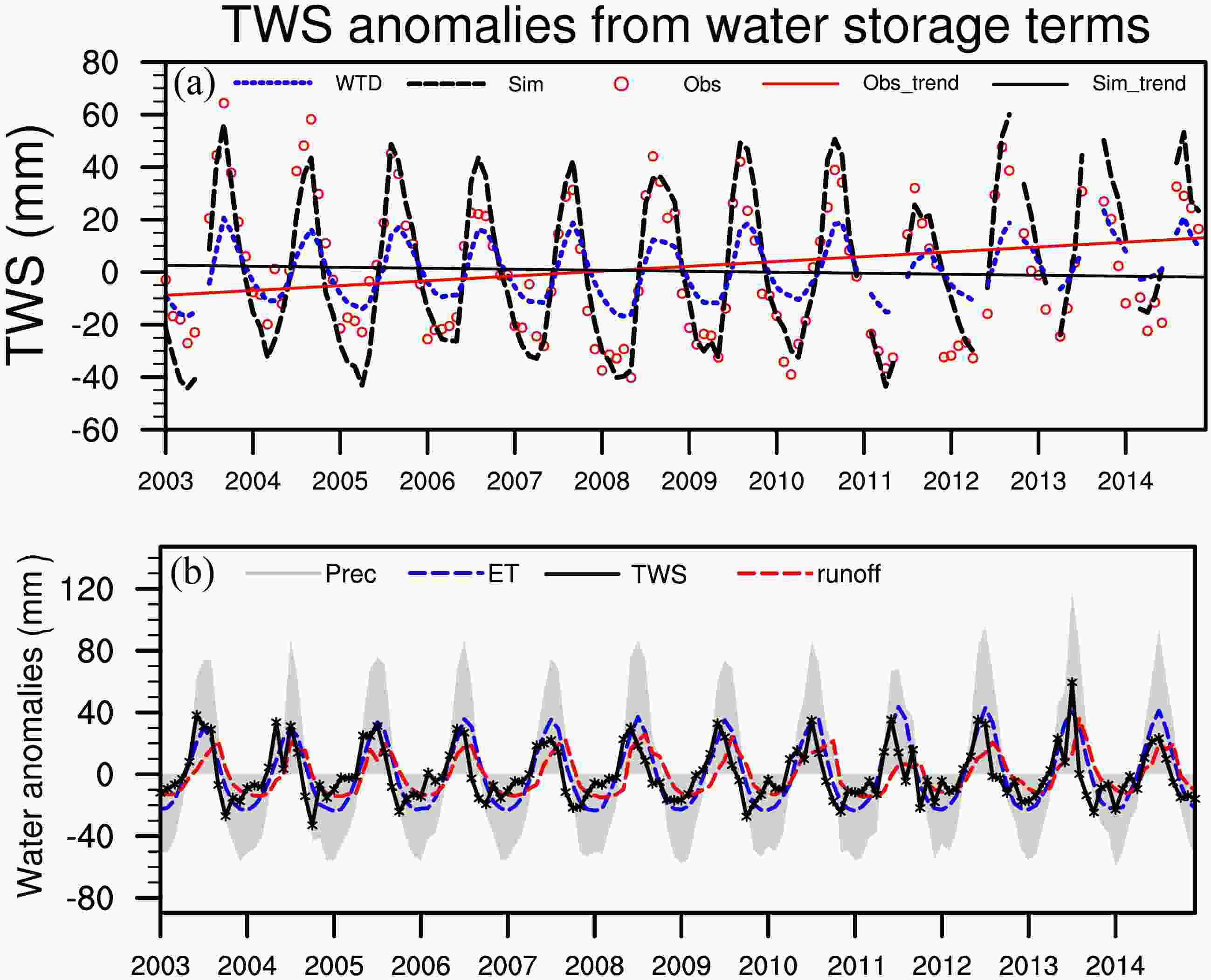 Figure7. TWS anomalies for China: (a) TWS calculated as the sum of three contributing components; and (b) the water flux terms, which are the cumulative results from three separate components.
| Region | R | RMSE (mm) | NSE |
| China | 0.76 | 20.29 | 0.46 |
| Yangtze River | 0.72 | 23.85 | 0.40 |
| Yellow River | 0.64 | 21.60 | 0.29 |
| Huaihe River | 0.80 | 32.42 | 0.40 |
| Haihe River | 0.83 | 23.88 | 0.72 |
| Pearl River | 0.92 | 23.03 | 0.67 |
| Songliao River | 0.64 | 31.91 | 0.23 |
Table6. Correlation coefficient (R), root-mean-square-error (RMSE), and Nash–Sutcliffe coefficient (NSE) for the monthly TWS anomalies between the simulation and GRACE data in different river basins from 2003 to 2014.
From the perspective of water flux, TWS is equal to the difference between precipitation and the sum of evapotranspiration and runoff. Figure 7b shows that the variation range of precipitation is the largest among all three components, implying its dominant role in controlling TWS among the water flux factors. Evapotranspiration and runoff are the second and third most important contributors, respectively.
To examine the ability of the simulation to model TWS under different climatic conditions, we evaluate the six river basins. Figure 8 shows that the simulation captures the variation in all the basins, with correlation coefficients greater than 0.7 (Table 6). In general, the simulations in the Pearl and Haihe Rivers are better, with correlation coefficients greater than 0.8 and NSE around 0.7. The Haihe, Huaihe, and Yellow Rivers were all affected by floods in 2003; these sudden increases in flow are reflected by both the simulation and the GRACE data. The Songliao River, which has the smallest variation, was affected by a drought event in 2007 and flooding in 2013; both of these incidents are well-traced by the simulation. The performance of the simulation still needs to be improved for the Yellow and Songliao Rivers, which could be partially explained by the complex topography and human activity over these regions.
 Figure8. Comparison of simulated and GRACE TWS anomalies from the water storage terms for the six major river basins in China.
The simulation captures the decreasing trend of TWS for the Huaihe River and the increasing trends for the Yangtze, Songliao, and Pearl Rivers. However, it underestimates the decrease in TWS for the Yellow and Haihe Rivers in recent years, overlapping with the time period of the greatest overexploitation of groundwater. The model only reflects the increase in precipitation during the experimental period, rather than the impact of human activity, which leaves room for improvement of the model.
2
3.5. Evaluation using Budyko’s aridity index
To further investigate the performance of the model under different climatic conditions, we evaluate the simulation of evapotranspiration and TWS with different Budyko’s aridity indexes, which is defined as the ratio of the annual potential evapotranspiration to the annual precipitation, with the expression of the former as the annual net radiation divided by the latent of heat of vaporization for water (Gerrits et al., 2009). Following the classification of Budyko’s aridity index, we divide China into three areas: a humid zone (aridity index < 1), a transitional zone (aridity index 1–2.25), and an arid zone (aridity index > 2.25) (Fig. 9a).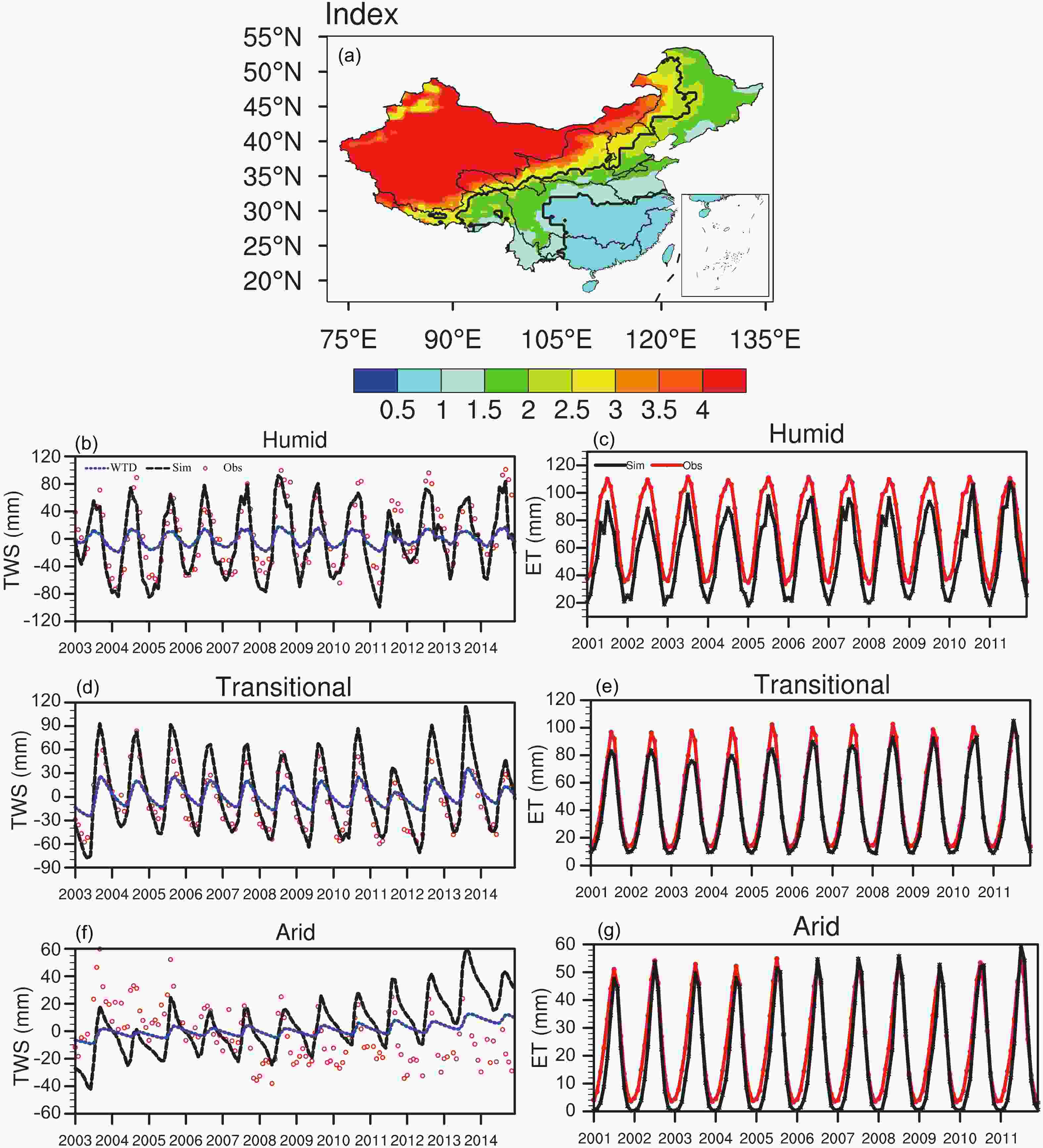 Figure9. (a) Spatial distribution of Budyko’s aridity index, where the black lines at 1.0 and 2.25 divide China into humid, transitional, and arid zones. (b, d, f) Comparison of the simulated TWS anomalies with GRACE estimates. (c, e, g) Comparison of the simulated evapotranspiration with FLUXNET estimates.
Figures 9b, d and f show that the simulation captures the variation in TWS in the humid and transitional zones, with an NSE greater than 0.6, but that the model needs to be improved to be able to reproduce the TWS in the arid zone during the same period. Specifically, increasing trends are seen in all three zones in the simulation as a result of the increase in precipitation in recent years. However, GRACE only shows the same increasing trend as the simulation in the humid zone, where there is no excessive exploitation of groundwater. The model is unable to reflect this phenomenon in the transitional and arid zones as a result of the lack of inclusion of the effects of human activity in the model, which therefore shows the opposite trend to the GRACE data.
Figures 9c, e and g indicate the ability of the model to capture the variation in evapotranspiration in all three zones, with correlation coefficients greater than 0.97. However, the simulation shows a clear underestimation in the humid zone, consistent with previously reported work (Lin et al., 2018b). The match between the simulation and the FLUXNET data gradually improves with increases in the aridity index, which may be explained by a simple mechanism of evapotranspiration in the arid regions with fewer plants. As the region becomes wetter and the fraction of vegetation increases, it is difficult to determine the dominant element in evapotranspiration with a more complicated mechanism because it is the sum of soil evaporation, canopy evaporation, and canopy transpiration. Vegetation does not change very much, meaning its fraction always keeps at a relatively high level, throughout the year, in the humid zone. In addition, the simulation underestimates the skin temperature. Both of these lead to the underestimation in the simulation over the whole time period. However, in the transitional zone, the amount of vegetation varies across the different seasons and the underestimation mainly occurs in summer. The underestimation is only observed in the cold season in the arid zone because frozen soil, which is sensitive to the soil temperature, makes it difficult for the model to reproduce evapotranspiration.
We find that the runoff scheme is the most important factor influencing the hydrological performance in averaged soil moisture, runoff, evapotranspiration, and their relationships (Fig. 10). There is an overall positive correlation between soil moisture and evapotranspiration and a negative correlation between evapotranspiration and runoff in the simulation. SIMTOP produces the highest evapotranspiration and soil moisture among the four runoff schemes because the model seals the soil bottom to retain more water in the soil, which may then become a source of water for evapotranspiration. The BATS scheme produces the smallest amount of evapotranspiration and soil moisture and the largest amount of runoff, which restricts the amount of water infiltrating the soil.
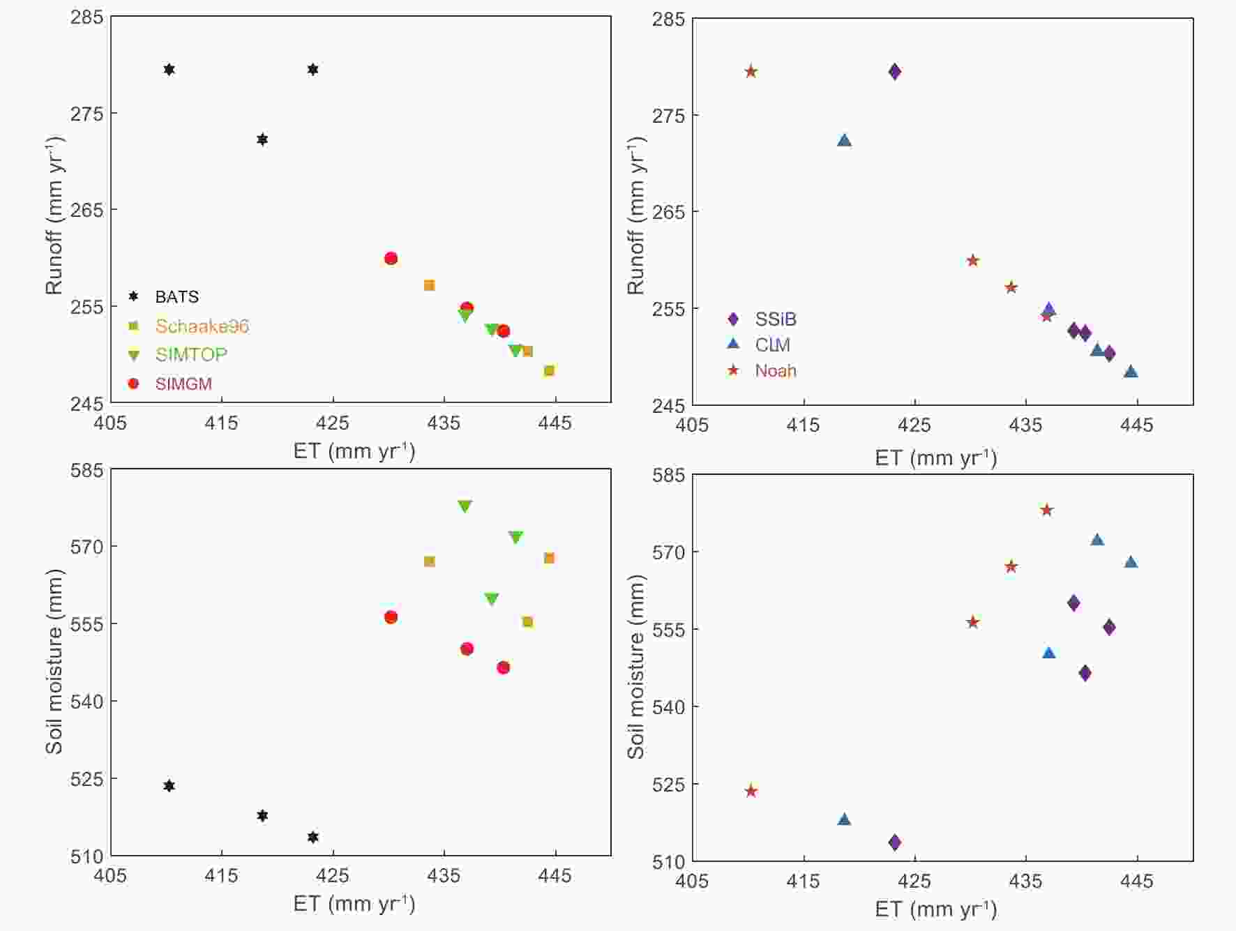 Figure10. Relationships between evapotranspiration and runoff (upper panels), and the top 2-m soil moisture versus evapotranspiration (lower panels). All variables are averaged over China for the period of 2001–14.
Given the same amount of soil moisture, both CLM and SSiB simulate more evapotranspiration than Noah because the former two use the same matric potential method. However, there are smaller differences in the simulations among the various stomatal resistance schemes than those resulting from the different runoff schemes, since the degree of impact of the stomatal resistance on the relationship between soil moisture and evapotranspiration should depend on the soil moisture regime, meaning that the stomatal resistance should exhibit more effects over the region with specific soil types and ranges of soil moisture than the national scale average (Yang et al., 2011).
As in Zheng et al. (2019), the runoff schemes show larger uncertainties than the stomatal resistance schemes when simulating the annual mean climatologies of soil moisture, evapotranspiration and runoff. We analyze monthly variations of soil moisture, evapotranspiration, and runoff in different schemes (shown in the supplementary material, Fig. S5). The above conclusion becomes clearer, especially for runoff. Specifically, the percentages of the ranges caused by the different runoff (stomatal resistance) schemes in the mean of all 12 experiments are around 30% (10%) for runoff, 8% (2%) for soil moisture, and 8% (2%) for evapotranspiration. The stomatal conductance and turbulence schemes may also show relatively large uncertainties in hydrological variables, which will be investigated in future work.
It should be acknowledged that there will be uncertainties in the observation data. The in-situ soil moisture data will not only contain errors from instruments and measuring practices, but also may not represent grid-mean states well. Most stations are located in the urban fringe area because of convenience, making the occurrence of sampling errors or human influence inevitable. Runoff data are a blended product of streamflow data and model simulations. As the model fails to represent the influence of human activities on runoff, it adds to the uncertainties in runoff data. FLUXNET-MTE-derived evapotranspiration data have uncertainties stemming from the sparse and uneven distributions in China, and are further contributed by the derivation of MTE. GRACE-derived TWS data have uncertainties in satellite measurements and post-processing. The influence of all these uncertainties on the evaluation needs to be explored in future work.
Overall, Noah-MP, with GLDAS forcing, simulates the hydrological variables for China reasonably well, showing its potential in flood and drought prediction studies and regional hydrological management. Notably, there is still quite a lot of room for improvement in the model, especially for TWS in regions with intense human activity (a likely result of groundwater exploitation), and for runoff in the Yellow and Liaohe River basins, located mostly in the semiarid region where lots of LSMs still struggle to reproduce the streamflow patterns and dynamics.
Acknowledgments. This work was supported by the National Key Research and Development Program of China (Grant No. 2018YFA0606004) and the National Natural Science Foundation of China (Grant Nos. 91337217 and 41375088). The first author acknowledges the support of the China Scholarships Council.
Electronic supplementary material: Supplementary material is available in the online version of this article at
Electronic Supplementary Material to: Systematic Hydrological Evaluation of the Noah-MP Land Surface Model over China*
Jingjing LIANG1, Zongliang YANG*2, and Peirong LIN2,3
1 Institute of Atmospheric Physics, Chinese Academy of Sciences, Beijing 100029, China2 Jackson School of Geosciences, University of Texas at Austin, Austin, TX 78712, USA3 Department of Civil and Environmental Engineering, Princeton University, Princeton, NJ 08540, USA
ESM to: Liang, J. J., Z. L. Yang, and P. R. Lin, 2019: Systematic hydrological evaluation of the Noah-MP land surface model over china. Adv. Atmos. Sci., 36(11), 1171?1187, https://doi.org/10.1007/s00376-019-9016-y.
