HTML
--> --> -->Because the output of NWP and observations have different systematic errors, the forecasting performance for various regions, seasons and weather processes is different. Before the release of a weather forecast, in order to further improve its accuracy, a weather consultation is indispensable. The forecasters obtain the final results during this weather consultation by combining observations with the NWP results and giving opinions based on their experience. The process of weather consultation is actually a manual process of post-processing the NWP results, and thus the professional knowledge and practical experience of individuals have a crucial impact on the forecast results. Owing to the current increase in data size and the improvement of weather forecasting requirements, the current weather consultation model cannot meet the needs of the development of weather forecasting, and so suitable post-processing algorithms are needed to help the manual process of weather consultation (Hart et al., 2003; Cheng and Steenburgh, 2007; Wilks and Hamill, 2007; Veenhuis, 2013).
In order to remove systematic errors and improve the output from NWP models, a variety of post-processing methods have been developed for simulating weather consultation (Wilks and Hamill, 2007; Veenhuis, 2013)—for example, model output statistics (MOS) (Glahn and Lowry, 1972; Cheng and Steenburgh, 2007; Wu et al., 2007; Glahn et al., 2009; Jacks et al., 2009; Zhang et al., 2011; Glahn, 2014; Wu et al., 2016), the analog ensemble (Monache et al., 2013; Alessandrini et al., 2015; Junk et al., 2015; Plenkovi? et al., 2016; Sperati et al., 2017), the Kalman filter (Delle Monache et al., 2011; Cassola and Burlando, 2012; Bogoslovskiy et al., 2016; Buehner et al., 2017; Pelosi et al., 2017), anomaly numerical-correction with observations (Peng et al., 2013, 2014), among which MOS is one of the most commonly used to produce unbiased forecasts (Glahn et al., 2009). MOS uses multiple linear regression to produce an improved forecast at specific locations by using model forecast variables and prior observations as predictors (Marzban et al., 2006; Cheng and Steenburgh, 2007). MOS remains a useful tool and, during the 2002 Winter Olympic Games, MM5-based MOS outperformed the native forecasts produced by MM5 and was equally or more skillful than human-generated forecasts by the Olympic Forecast Team (Hart et al., 2003). Glahn (2014) used MOS with a decay factor to predict temperature and dewpoint, and showed how different values of the decay factor affect MOS temperature and dewpoint forecasts (Glahn, 2014).
Although machine learning and statistics both draw conclusions from the data, they belong to two different modeling cultures. Statistics assumes that the data are generated by a given stochastic data model. Statistical methods have few parameters, and the values of the parameters are estimated from the data. Machine learning uses algorithmic models and treats the data mechanism as unknown. The approach of machine learning is to find an algorithm that can be fitted to the data, and it has lots of parameters (Breiman, 2001b). Machine learning has developed rapidly in fields outside statistics. It can be used both on large complex datasets and as a more accurate and informative alternative to data modeling on smaller datasets (Mirkin, 2011). Machine learning is becoming increasingly more important to the development of science and technology (Mjolsness and Decoste, 2001). To apply machine learning to practical problems, one of the most important things is to apply feature engineering and data structures (Domingos, 2012). The quality of feature engineering directly affects the final result. For some practical problems with special data structures, targeted feature engineering is required.
Since weather forecasts depend highly on data information and technology, how to make better use of machine learning and big-data technology to improve weather forecasts has become a research hotspot. Machine learning has been used in meteorology for decades (Haupt et al., 2009; Lakshmanan et al., 2015; Haupt and Kosovic, 2016; Cabos et al., 2017). For instance, the neural network technique was applied to the inversion of a multiple scattering model to estimate snow parameters from passive microwave measurements (Tsang et al., 1992). Schiller and Doerffer (1999) used a neural network technique for inverting a radiative transfer forward model to estimate the concentration of phytoplankton pigment from Medium Resolution Imaging Spectrometer data (Schiller and Doerffer, 1999). Chattopadhyay et al. (2013) put forward a nonlinear clustering technique to identify the structures of the Madden?Julian Oscillation (Chattopadhyay et al., 2013). Woo and Wong (2017) applied optical flow techniques to radar-based rainfall forecasting (Woo and Wong, 2017). Weather consultation data are unique, and mainly include NWP model data and observational data. They have different data structures and features, which makes feature engineering a complicated task. On the one hand, the observational data are real, but they only comprise the historical data of weather stations. If relying solely on observational data for prediction, only short-term weather can be predicted. On the other hand, model data reflect the average of a region, and can therefore help to make long-term predictions. Furthermore, model data have time series and a spatial structure that contain abundant intrinsic information on the problem to be solved.
Therefore, the key to using machine learning algorithms to solve the problems of weather forecasts is to apply feature engineering, such that the structure of observational and model data can be fully taken into account. This is a difficult but meaningful topic.
The ever-increasing demand for weather forecasts has made the accuracy of grid weather forecasts more and more important. However, most post-processing methods, such as MOS, can only consider the correction of one spatial point, without considering the spatial and temporal structure of the grid. Currently, one challenging and important area of research is finding a solution to apply post-processing methods to large volumes of gridded data across large dimensions in space and time. The feature engineering of constructing a data structure is a useful technology to achieve this goal.
In this paper, the model output machine learning (MOML) method is proposed for simulating weather consultation. MOML matches NWP forecasts against a long record of verifying observations through a regression function that uses a machine learning algorithm. MOML constructs datasets by feature engineering based on spatial and temporal data, and it can make full use of the spatial and temporal structure of a point on the grid. In order to test the results of the application in practical problems, the MOML method is used to forecast 2-m grid temperature in the Beijing area. A variety of post-processing methods are used to calculate the 2-m temperature with different datasets in a 12-month period, including several machine learning algorithms, such as multiple linear regression and Random Forest, two training periods, and three datasets.
The paper is organized as follows: In section 2, the data and the problem concerned in this study are described. The MOML method is proposed in section 3. Section 4 compares the NWP forecasts with the numerical results from multiple linear regression, Random Forest, and MOS. Conclusions are drawn in section 5.
2.1. Model data
The six-hourly forecast data of the ECMWF model initialized at 0000 UTC up to a lead time of 360 hours from January 2012 to November 2016 are used in this paper. The model data are obtained for a grid of 5 × 6 points covering the Beijing area (39°?41°N, 115°?117.5°E) with a horizontal resolution of 0.5°, as well as the grid points on the edge of this area, and thus the model data on this 7 × 8 grid are used. Several predictors (e.g., land?sea mask) have the same value in the Beijing area and do not change with time. In addition to these unnecessary variables, 21 predictors are chosen, broadly based on meteorological intuition. Table 1 shows these predictors and their abbreviations.| Predictor | Abbreviation |
| 10-m zonal wind component | 10U |
| 10-m meridional wind component | 10V |
| 2-m dewpoint temperature | 2D |
| 2-m temperature | 2T |
| Convective available potential energy | CAPE |
| Maximum temperature at 2 m in the last 6 h | MX2T6 |
| Mean sea level pressure | MSL |
| Minimum temperature at 2 m in the last 6 h | MN2T6 |
| Skin temperature | SKT |
| Snow depth water equivalent | SD |
| Snowfall water equivalent | SF |
| Sunshine duration | SUND |
| Surface latent heat flux | SLHF |
| Surface net solar radiation | SSR |
| Surface net thermal radiation | STR |
| Surface pressure | SP |
| Surface sensible heat flux | SSHF |
| Top net thermal radiation | TTR |
| Total cloud cover | TCC |
| Total column water | TCW |
| Total precipitation | TP |
Table1. The predictors taken from the ECMWF model and their abbreviations.
These model data constitute a part of the original dataset D0, and this part is denoted by X0. A record of meteorological elements on a certain day at a spatial point is called a sample S, and thus there are 1796 samples, i.e., S = 1, 2, …, 1796. Each sample has 61 six-hour time steps TTem with a forecast range of 0?360 hours (TTem= 0, 6, …, 360) and 21 predictors C, as listed in Table 1

2
2.2. Observational data
Data assimilation can determine the best possible atmospheric state using observations and short-range forecasts. The weather forecasts produced at the ECMWF use data assimilation and obtain the model analysis (zero-hour forecast) from meteorological observations. Therefore, for this study, the model analysis is used as the label, because not every grid point has an observation station. Furthermore, the model analysis data contain the observational information through data assimilation. The model analysis data used in this paper are the 2-m temperature of the ECMWF analysis in the Beijing area, with a horizontal resolution of 0.5° and recorded every 0000 UTC from 1 January 2012 to 15 December 2016.These observational data constitute the other part of the original dataset D0, and this part is denoted by Y0, D0 = (X0, Y0). Following the above notation, the samples S = 1, 2, …, 1796 are from January 2012 to November 2016, the predictor C is given the value 2T, 2T stands for 2-m temperature, the horizontal grid division is 5 × 6, and thus m = 2, 3, …, 6 and n = 2, 3, …, 7. Actually, the model analysis data include 1811 days, because, for a sample, the temperatures in the next 15 days are predicted by the model, and the corresponding true values need to be used. Let t be the forecast lead time, t = 24, 48, …, 360 hour, for a fixed (m, n) and S, the temperatures in the next t hours can be aggregated into vectors. Y0 can be written as
where C = 2T was omitted. Y0 consists of a 4D array, of which the size is 1796 × 5 × 6 × 15.
2
2.3. Problem
For this study, the grid temperature forecast is actually a problem of using the predictions from the ECMWF model as the input and obtaining the 2-m grid temperature forecasts as the output. Focusing on the samples from January to November 2016, for each sample, the 2-m grid temperature forecasts in the Beijing area at the forecast lead times of 1?15 days need to be forecast.3.1. Univariate linear running training period MOS
Univariate linear MOS is one of the most important and widely used statistical post-processing methods (Glahn and Lowry, 1972; Marzban et al., 2006). The statistical method used by univariate linear MOS is unary linear regression; thus, only one predictor is used. The general unary linear regression equation of univariate linear MOS can be written aswhere y is the desired predicted value; xp is the predictor, which is the NWP model output of this predicted value; w0 is the intercept parameter, and w1 is the slope parameter of the linear regression equation. Applying univariate linear running training period MOS to this problem, for a fixed (m, n, t) and S, the predicted value


2
3.2. Machine learning
The meaning of machine learning in terms of weather forecasting can be understood in conjunction with the data mentioned above. In machine learning, a feature is an individual measurable property or characteristic of a phenomenon being observed, and a label is resulting information (Bishop, 2006). Machine learning obtains a model f by learning in the training set (Xtrain, Ytrain). Then, for a test sample in the test set, its predicted value


Using the MOML method to solve the problem raised in section 2.3, the most important step is feature engineering. Feature engineering produces different datasets, and then a machine learning algorithm is used to process these datasets. As we all know, in order to obtain better results, the importance of feature engineering is far greater than that of the choice of machine learning algorithm. Therefore, this paper focuses on feature engineering in MOML (section 2.3), and two mature machine learning algorithms are used.
3
3.2.1. Multiple linear regression
Multiple linear regression attempts to model the relationship between two or more explanatory features and a response variable by fitting a linear equation to observed data. In this problem, a multiple linear regression model with d features

which can also be written in the vector form


Multiple linear model is a simple but powerful model to solve problems. The coefficient can intuitively express the importance of each independent normalized feature, which means the multiple linear model is an explanatory model.
3
3.2.2. Random Forest
A decision tree is a tree-like structure in which each internal node represents a test on an attribute, each branch represents the output of the test, and each leaf node represents a class label (Alpaydin, 2014). Decision trees can be classified into classification trees and regression trees. This problem is a regression problem, and thus a regression tree is used. A regression tree generation algorithm that can be applied to this problem is depicted in Fig. 1.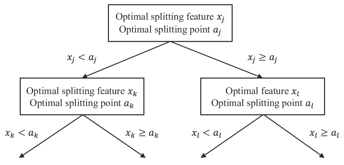 Figure1. Diagram of a regression tree generation algorithm, where xj is the optimal splitting features and aj is the optimal splitting point.
This regression tree generation algorithm chooses the optimal splitting features xj and the optimal splitting point aj, and solves
where


In this problem, a regression tree f is generated with the features


The bagging decision tree algorithm is an ensemble of decision trees trained in parallel, and the Random Forest algorithm is an extended version of the bagging decision tree algorithm, which introduces random attribute selection in the training process of the decision tree (Breiman, 2001a).
Actually, the dataset is divided into a training set and test set, and the training set is also randomly divided into a training subset and validation subset. The training subset and validation subset used in the Random Forest algorithm are generated by the random selection of bagging from the training set (Breiman, 2001a). The test set is used to test the results of the algorithm.
Random Forest has low computational cost and shows strong performance in many practical problems. The diversity of the base learners in Random Forest is not only from the sample bagging, but also from the feature bagging, which enables the generalization performance of the final ensemble algorithm to be further improved by the increase in the difference among the base learners.
2
3.3. MOML method
MOML is a machine learning-based post-processing method, which matches NWP forecasts against observations through a regression function, and improves the output of the ensemble forecast. The MOML regression function uses an existing machine learning algorithm. Setting the MOML regression function as f, the MOML regression equation is written aswhere


This MOML method involves performing two steps: feature engineering and machine learning.
First, by utilizing feature engineering (sections 3.3.1 and 3.3.2), the original dataset D0 = (X0, Y0) needs to be processed into the training set (Xtrain, Ytrain) and the test set (Xtest, Ytest) to fit machine learning. The test set can be obtained by dividing the samples; when S = 1442, 1443…, 1796, the data are in the test set. The feature engineering focuses on two aspects: the training period and the dataset.
On the one hand, for training set selection, the samples of the original training set are S = 1, 2…, 1441, and for each sample S in the test set there are different ways to select the training period to construct the training set. For this study, the original training set can be improved to some training periods that are more suitable for this problem (example in section 3.3.1).
On the other hand, for a sample S at fixed (m, n, t) in this problem, the label


Second, by using the machine learning regression function f and the training data, the parameter

where argmin stands for arguments of the minimum, and are the points of domain of some function at which the function values are minimized, and the machine learning regression function f and the parameter

The flow diagram of the MOML method is shown in Fig. 2. The MOML diagram uses multi-layer structures to represent historical time series. The extracted square of the diagram refers to selecting the required data from all the features to form predictors on the one hand, and on the other hand it represents the spatial structure around a single grid point. MOML can calibrate not only the forecasts of a single point, but also those of all points on the grid by constructing a suitable dataset. Feature engineering is the first and most important step of MOML, which includes the processing of both the training period and datasets. In terms of the training period, a year-round training period and running training period are considered. For datasets, temporal and spatial grid data are considered and combined into three datasets.
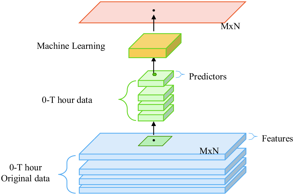 Figure2. Flow diagram of the MOML method. The blue cuboids are the original data in the Beijing area, and the green cuboids are the dataset with proper feature engineering. The yellow cuboid represents the process of machine learning, and the orange rectangle represents the output.
3
3.3.1. Feature engineering: training period
The data of 366 days (from 1 December 2015 to 30 November 2016) from those of 1827 days (from 1 January 2012 to 30 November 2016) from the ECMWF model are taken as the test set, i.e.,The training period is a set of times throughout the original training set, and the training set in this problem concerns the following two types of training period.
3
3.3.1.1. Year-round training period
One of the most natural ideas is for any month on the test set, all the previous data are taken as the training set. For example, when the temperatures from 1 February to 29 February 2016 need to be forecast, the training period is 1 January 2012 to 31 January 2016. This training period is named as the year-round training period. This training period is simple and suitable for most machine learning algorithms, but the training period is fixed for some samples.3
3.3.1.2. Running training period
Some optimal training periods have been proposed in recent years. Wu et al. (2016) used the running training period scheme of MOS to forecast temperature (Wu et al., 2016). The idea of the running training period is that, for any day on the test set, the data for 35 days before the forecast time and 35 days before and after the forecast time for previous years are taken as a training set. For example, when the temperature of 1 May 2016 needs to be forecast, the training period is from 27 March to 30 April 2016 and from 27 March to 5 June 2012?15. This training period can be adjusted as the date changes.3
3.3.2. Feature engineering: dataset
The original dataset D0 = (X0, Y0) is reconstituted into datasets 1?3 separately, Di = (Xi, Yi), i = 1, 2, 3. The labels of datasets 1 and 2 are the same as that of the original data set, i.e.,The features are different according to diverse ways of dealing with the spatial structure.
3
3.3.2.1. Dataset 1
For the label


if t ≤ 60, TTem = 0, 6…, t. Then, reshape the array


if t ≤ 60, TTem = 0, 6…, t. Then, reshape the array


and dataset 2 D2 = (X2, Y2). Figure 3b depicts dataset 2 diagrammatically.
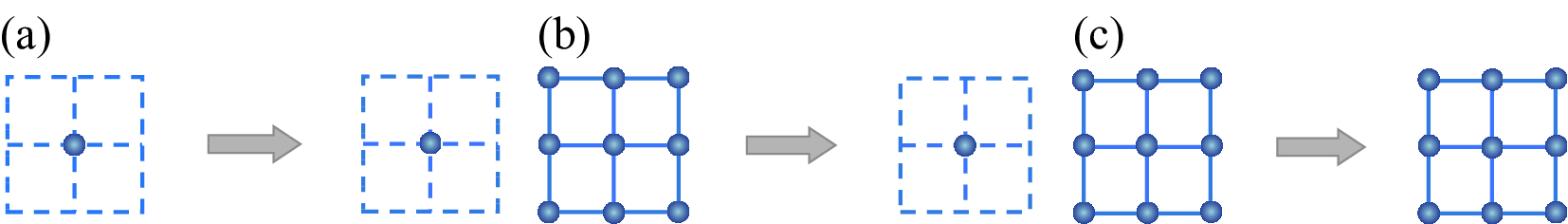 Figure3. Diagram of datasets 1?3. Dataset 1 focuses on the fixed spatial point, and dataset 2 adds the surrounding eight grid points. Dataset 3 takes all the 30 spatial points of the Beijing area into account in a unified way.
and dataset 1 D1 = (X1, Y1). Figure 3a depicts dataset 1 diagrammatically.
3
3.3.2.2. Dataset 2
For the label


3
3.3.2.3. Dataset 3
By using the idea of spatial interpolation, for a fixed spatial point (m, n), the longitude, latitude and altitude of the grid point are uniquely determined (m = 2, 3…, 6 and n = 2, 3…, 7). At a fixed forecast time tth hour (
Then, add the longitude, latitude and altitude of the 30 spatial points as the new predictors to the features

if t ≤ 60, TTem= 0, 6…, t. Then, reshape the array


if t ≤ 60, TTem = 0, 6…, t. Also, we have
and dataset 3 D3 = (X3, Y3). Figure 3c depicts dataset 3 diagrammatically.
The RMSE is one of the most common performance metrics for regression problems, and the RMSE of temperature is denoted by TRMSE,
where f is the machine learning regression function, D is the dataset, K is the total number of samples of dataset D, xk is the input, and yk is the label.
The temperature forecast accuracy (denoted by Fa) in this study is defined as the percentage of absolute deviation of the temperature forecast not being greater than 2°C,
where Nr is the number of samples in which the difference between the forecast temperature and the actual temperature does not exceed ±2°C and Nf is the total number of samples to be forecast.
In this section, the MOML method with the multiple linear regression algorithm (“lr”) and Random Forest algorithm (“rf”) is used to solve the problem of grid temperature forecasts, mentioned in section 2.3, and datasets 1?3 with two training periods, a year-round training period and running training period, are adopted. It is worth noting that the multiple linear regression algorithm is unsuitable for dataset 2 because it has too many features, and the running training period is unsuitable for Random Forest because of the heavy computation. The univariate linear MOS method is a linear regression method that uses only temperature data and does not require the datasets introduced in the last section. In fact, dataset 1 contains 21 features, dataset 2 contains 2268 features, and multiple linear regression is used on datasets 1 and 2 to obtain models


| Method | Dataset | Training period | Notation |
| ECMWF | ? | ? | ECMWF |
| Univariate linear MOS | ? | Running | mos_r |
| MOML (lr) | 1 | Year-round | lr_1_y |
| 3 | Year-round | lr_3_y | |
| 3 | Running | lr_3_r | |
| MOML (rf) | 2 | Year-round | rf_2_y |
| 3 | Year-round | rf_3_y |
Table2. List of methods used and their notation.
2
4.1. Whole-year comparison of the ECMWF model, univariate linear running training period MOS, and MOML
In this subsection, a whole-year comparison of the ECMWF model, univariate linear running training period MOS, and MOML is presented. The results of MOML with the multiple linear regression algorithm,

 Figure4. Results of the


Actually, the better the model data, the better the forecast results. The forecast accuracy is negatively correlated with the RMSE. Generally speaking, the lower the RMSE, the higher the forecast accuracy. The forecast ability of the model decreases linearly in a short time period, and nonlinearly in a long time period.
According to Fig. 4, all of the three methods (


 Figure5. A feasible solution fMOML to the grid temperature correction in the Beijing area. fMOML uses the

The average TRMSE and Fa of the solution fMOML and the ECMWF model (or univariate linear MOS) are calculated respectively, and these values are then used to evaluate the difference between the forecasting abilities of the two methods. In conclusion, the average TRMSE and average Fa of the solution for the fMOML method decreases by 0.605°C and increases by 9.61% compared with that for the ECMWF model, respectively, and by 0.189°C and 3.42% compared with that of the univariate linear running training period MOS, respectively.
2
4.2. Month-by-month comparison of the three algorithms
Considering that the change in temperature is seasonal within a year and fierce in some months in the Beijing area, a month-by-month comparison of the ECMWF model, univariate linear running training period MOS (

3
4.2.1. Winter months
It is more important to improve the accuracy of temperature forecasts in winter, because the forecast results of the ECMWF model do not work well in winter months. The forecast data in winter months are revised by the six methods listed in Table 2. Figure 6 shows the correction results of the grid temperature data in the Beijing area in November, December, January and February.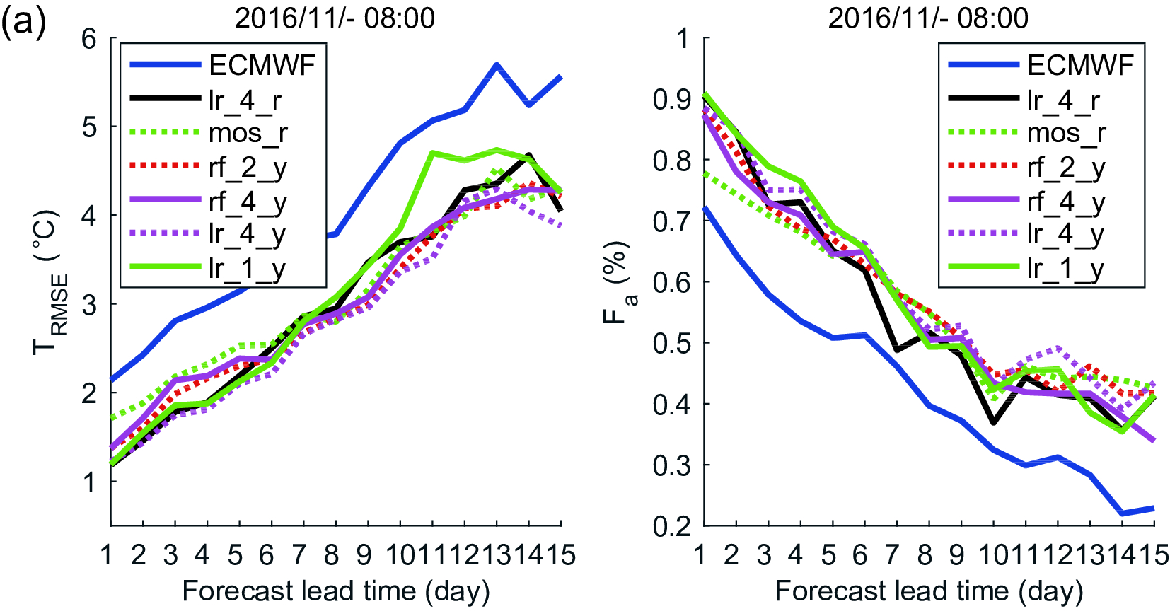 Figure6. Results of grid temperature forecasts in the Beijing area in November (a), December (b), January (c) and February (d). In these months, the forecast results of the ECMWF model do not work well, and the linear methods
From December to February, the average TRMSE and average Fa of the


3
4.2.2. Other months
Figure 7 shows the results of the grid temperature data in the Beijing area in March, June, July, August and October. In these five months, the forecast result of the ECMWF model are better than those in winter months, and the results of some MOML methods do not work better than the ECMWF model. On the whole, in these months, the results of MOML with the multiple linear regression algorithm are better than those of other methods in the first few days of the forecast period, and those with Random Forest are better than other methods when the forecast time is relatively long. Also, the results of the running training period are better than those of the year-round training period when applying a linear method.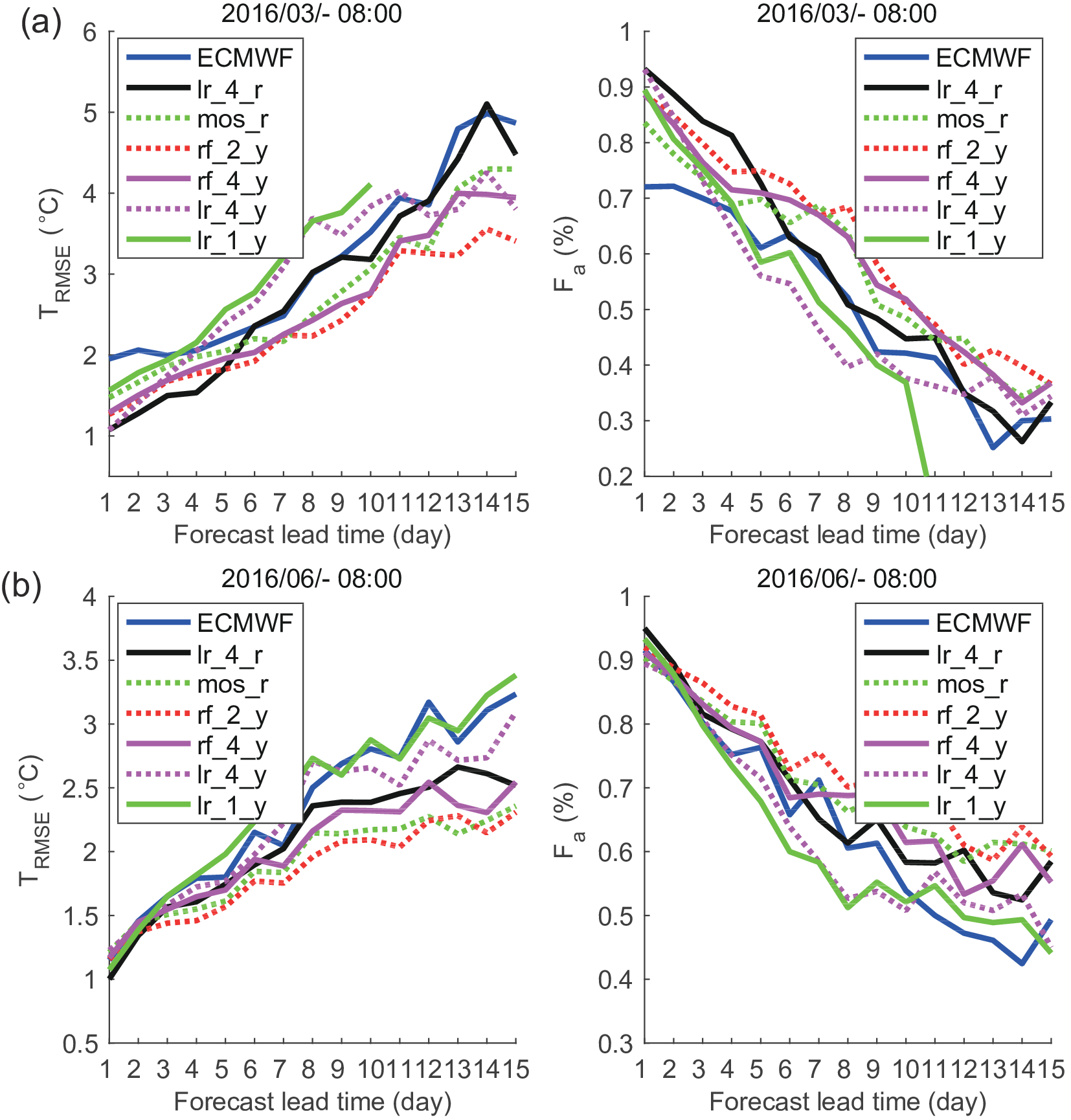 Figure7. Results of grid temperature forecasts in the Beijing area in March (a), June (b), July (c), August (d) and October (e). In these five months, the forecast results of the ECMWF model are better than those in winter months. The linear methods are better than other methods when the forecast lead time is short, and Random Forest algorithm are better when the forecast lead time is relatively long.
Figure 8 shows the correction results of the grid temperature data in Beijing in April, May and September. The forecast results of the ECMWF model in these three months are better than those in the other months, and there is no need for revision in selected times of the forecast period. On the whole, in these three months, the results of MOML with the multiple linear regression algorithm are best in the first few days of the forecast period, and those with the Random Forest algorithm are better than for other methods in the next few days. Also, the results of the running training period are close to those of the year-round training period when applying a linear method.
 Figure8. Results of grid temperature forecasts in the Beijing area in April (a), May (b) and September (c). In these three months, the forecast results of the ECMWF model in these three months are better than those in the other months. The multiple linear regression algorithm is best in the first few days of the forecast period, and the Random Forest algorithm is better than for other methods in the next few days.
In summary, the MOML method is better than the univariate linear running training period MOS method with a running training period, and has the ability to improve grid temperature forecast results in the Beijing area. In addition, as a post-processing method, MOML can be applied to the weather consultation process. This approach has good application prospects and can greatly reduce the manpower consumption during the consultation. In terms of its practical applicability, the machine learning algorithm in this paper adopts a mature, fast, multiple linear regression algorithm and the Random Forest algorithm, which do not need a lot of parameter adjustment and are easy to use. Constructing a more accurate and efficient machine learning algorithm to solve the problem will be our focus in future work.
Acknowledgments. The authors would like to express sincere gratitude to Lizhi WANG, Quande SUN and Xiaolei MEN for unpublished data; Zongyu FU and Yingxin ZHANG for professional guidance; and Zhongwei YAN and Fan FENG for critical suggestions. This work is supported by the National Key Research and Development Program of China (Grant Nos. 2018YFF0300104 and 2017YFC0209804) and the National Natural Science Foundation of China (Grant No. 11421101) and Beijing Academy of Artifical Intelligence (BAAI).
