HTML
--> --> -->There are two main downscaling approaches: dynamical downscaling and statistical downscaling. In the former, a higher-resolution model, such as a regional climate model (RCM), is driven by a GCM or reanalysis data and run at spatial resolutions of up to a few meters (e.g., Aitken et al., 2014), at which complex topography and smaller-scale processes are better represented (Laprise, 2008). This approach can give a very good simulation of local atmospheric conditions (Pan et al., 2012; Soares et al., 2012; Warrach-Sagi et al., 2013; Aitken et al., 2014; Heikkil? et al., 2014). However, it has some drawbacks: e.g., it requires a significant amount of computational resource, particularly for very-high-resolution simulations, and the RCM performance is also strongly dependent on the GCM/reanalysis boundary forcing data (Fowler et al., 2007). Further, when forced with coarse-resolution data and run without any additional constraints, the interior fields of the RCM’s domain can diverge substantially from the driving fields (e.g., Bowden et al., 2012, 2013). One way to prevent this is to relax or nudge the fields in the interior of the domain to those of the coarse-grid data used to force the model (e.g., Waldron et al., 1996; von Storch et al., 2000). However, doing so is not the meteorological community’s consensus, as it removes freedom from the model’s large scales (e.g., Miguez-Macho et al., 2004; Alexandru et al., 2009), even though it has proven to be effective (e.g., Otte et al., 2012). There are two main nudging techniques employed in RCMs: grid (or analysis) nudging and spectral nudging. In the former, the prognostic variables are relaxed towards a reference state at every grid point (e.g., Stauffer and Seaman, 1990), whereas in the latter only some zonal and meridional wavenumbers are retained, with all other waves filtered out (e.g., Miguez-Macho et al., 2004, 2005). Both techniques have been successfully applied in numerical simulations (e.g., Soares et al., 2012; Heikkil? et al., 2014; Steinhoff et al., 2014; Ma et al., 2016; Wootten et al., 2016).
A computationally less demanding and more flexible alternative to dynamical downscaling is statistical downscaling. Statistical methods have been used for some time to downscale and predict variables such as temperature and precipitation, and range from simple regression methods [including multiple linear regression and partial least-squares regression (e.g., Ke et al., 2011; Fan et al., 2012)] to more complex techniques such as singular value decomposition (e.g., Landman and Tennant, 2000; Wei and Huang, 2010), artificial neural networks (e.g., Wilby and Wigley, 1997), and the method of analogs (e.g., Zorita and von Storch, 1999).
Statistical techniques are often used to correct GCM/RCM parameter field biases (Déqué, 2007; Pierce et al., 2015). They are typically applied in a two-step process: in step (1), known as the past or “training” period, the statistical relationships between local climate variables (e.g., from a weather station) and large-scale fields (e.g., from a numerical model) are developed; and in step (2), known as the future or “prediction” period, they are applied to some period of interest. For example, model data for the past climate can be used for “training” purposes with the statistical relationships then applied to the output of the same model for a future climate simulation, to infer the local climate change signal (Diaz-Nieto and Wilby, 2005). As discussed in Pierce et al. (2015), some of the most commonly employed statistical techniques make use of the cumulative distribution functions (CDFs) of modelled and observed data. A CDF, denoted as FX(x), is a distribution function of a random variable X evaluated at xthat returns the probability of X≤x. It varies between 0, at the minimum value of a CDF, and 1, at its maximum value. When two CDFs are plotted against each other, a quantile-quantile (Q-Q) plot is obtained (Field, 2013). A simple bias correction approach is quantile mapping. In this technique, the Q-Q plot for the “training” period, obtained using past model and observational data, is used to bias-correct the model forecasts for the “prediction” period. Another commonly used method is equidistant quantile matching. Here, and at a given quantile, the model-predicted change signal is added to the observed data for the past period. The advantage of this approach is that, if the model bias is invariant with time, it will be effectively removed when taking the difference of the future and past forecasts. The statistical method used in this work is the CDF-transform, or CDF-t (Michelangeli et al., 2009). In this technique, a transformation that projects the model’s CDF to the observed CDF is computed over the past period and is subsequently applied to the model’s future CDF. This statistical stationarity assumption (invariance of statistical moments in time) is commonly made in CDF-t studies, including this one, even though it has recently been challenged (Dixon et al., 2016).
The CDF-t method has been used in a wide range of studies. It has been employed to directly downscale reanalysis data (Kallache et al., 2011), and it has also been applied in conjunction with a dynamically downscaled (GCM/RCM) product [hybrid technique (e.g., Lavaysse et al., 2012; Vrac et al., 2012; Flaounas et al., 2013; Wu et al., 2018)]. The CDF-t approach has been found to be very effective at removing model biases (e.g., Famien et al., 2018). In fact, Colette et al. (2012) concluded that a hybrid downscaling technique, using the Weather Research and Forecasting (WRF) model (Skamarock et al., 2008) and the CDF-t approach, can give nearly unbiased, high-resolution, physically consistent, three-dimensional fields that can be used for climate impact studies. Vigaud et al. (2013) applied the CDF-t to GCM surface temperature and precipitation predictions over southern India. The authors found a substantial improvement compared to the raw GCM data, regarding the distribution, seasonal cycle and monsoon daily means for different environments in the Indian subcontinent. Bechler et al. (2015) downscaled WRF-predicted precipitation data over southern France using different hybrid downscaling approaches and found that CDF-t was one of the best performing statistical techniques. The successful implementation of the CDF-t for different meteorological studies, such as those mentioned above, justifies the choice of the technique for this work.
In this paper, the CDF-t technique is first developed using the 3-km output of the WRF model, WRF[3 km], and station data from the Finnish Meteorological Institute (FMI). For the central month of each season in a given year, the developed technique is used in combination with a 3-km WRF output, with the hybrid statistical–dynamical downscaling, WRF[3 km]+CDF-t, compared against a 1-km dynamically downscaled product, WRF[1 km], over Scandinavia. If WRF[3 km]+CDF-t is found to give more accurate predictions than WRF[1 km], it can be argued that there is no substantial added value in conducting numerical simulations over this region at kilometer and perhaps sub-kilometer resolutions. Should this be true, and given that a very-high-resolution dynamical downscaling is extremely computationally expensive, the findings of this work will provide guidance into the setup of future model runs over Scandinavia.
The focus of the work is on the air temperature as (i) it is a crucial field for the vast majority of weather and climate applications, including climate change studies (e.g., Overland et al., 2016), and (ii) this variable is projected to change significantly in the target region in a hypothetical warming climate (e.g., Jylha et al., 2004; Hanssen-Bauer et al., 2005). In addition, RCMs, including the WRF model, are found to have large temperature biases in the region (e.g., Kotlarski et al., 2014; Katragkou et al., 2015), making it of interest to investigate how much of an added value a hybrid downscaling approach will give.
This paper is organized as follows. The models, datasets and diagnostics are introduced in section 2. The results are presented and discussed in section 3, while the main findings are outlined in section 4.
2.1. WRF simulations
In this study, the WRF model is run over the Honkajoki wind farm in near-coastal western Finland with two different configurations, given in Fig. 1. For the “training” period, a 20-year run (April 1997 to March 2016) with 27-, 9- and 3-km grids is conducted, hereafter referred to as the WRF[3 km] simulation. For the “forecast” period, WRF is run for 4 months (April, July, October 2016 and January 2017) with an additional 1-km nest, WRF[1 km]. The computational cost of the WRF[1 km] simulations hinders us from taking full seasons as prediction periods, so we focus instead on the central month of each season. The rather short evaluation period is a limitation of this study, and a multi-year simulation would be needed given the significant interannual variability of the atmospheric conditions in northern Europe (e.g., Toniazzo and Scaife, 2006; Gray et al., 2016). The Honkajoki near-coastal region is selected given its strong seasonal contrast, typical of high-latitude climates (snow-covered terrain and coastal sea-ice in winter versus open water and snow-free land in summer). The presence of a wind park in this area provides a potential extension of the methodology developed here for wind-energy-related applications. Figure 1 shows the spatial extent of the model grids used in both simulations: 27-9-3 km grids in the former, and 27-9-3-1 km grids in the latter. The initial and boundary conditions for the runs are obtained from the National Centers for Environmental Prediction Climate Forecast System Reanalysis (CFSR; Saha et al., 2010) 6-hourly data (spatial resolution of 0.5° × 0.5°). CFSR has been shown to be one of the best performing reanalysis datasets in midlatitude environments (e.g., Ebisuzaki and Zhang, 2011; Free et al., 2016). It is important to note that the spatial resolution of the CFSR data is higher than that employed in the majority of GCMs used for climate simulations: e.g., the output of the Community Climate System Model, version 3 (Collins et al., 2006), frequently used to drive future regional climate change simulations, is available at a 1.4° spatial resolution (Bruyère et al., 2014). CFSR data are employed here to force WRF owing to their good performance over the region, and given that the focus of this work is on the assessment of the performance of the two downscaling methods. In order to minimize the accumulation of integration errors, and following Lo et al. (2008), the simulations are broken into several overlapping periods. For the 20-year WRF simulation, WRF[3 km], the model is run for 13 months at a time (March year Z to March year Z+1) with the first month regarded as model spin-up. The (re-)initialization takes place in spring so as to keep the summer (June to August) and winter (December to February) seasons within one continuous integration. The WRF[1 km] simulations are conducted separately for April 2016 (spring), July 2016 (summer), October 2016 (autumn) and January 2017 (winter), with a 1-day spin-up before each.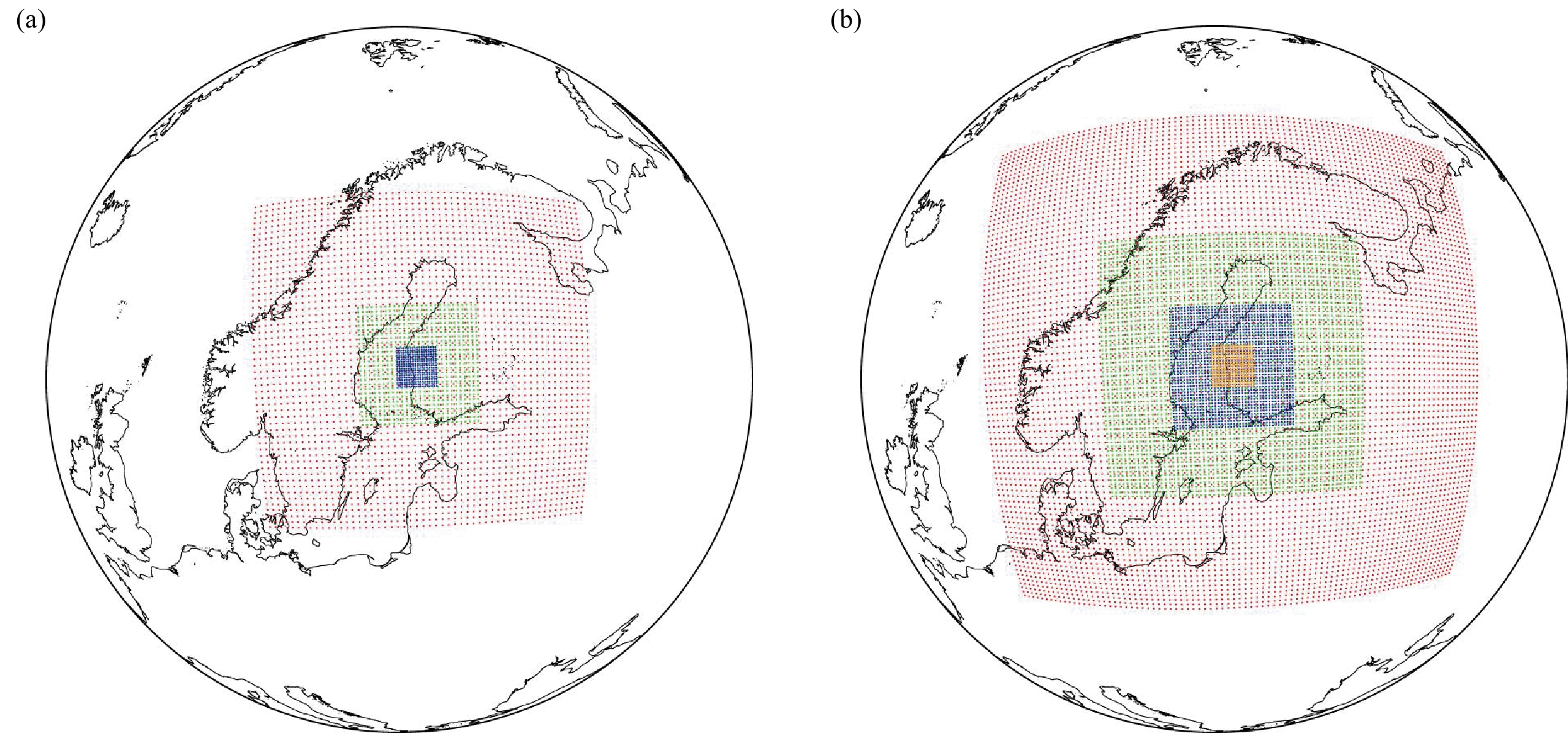 Figure1. Spatial extent of the model grids used in the (a) 20-year and (b) 1-year WRF simulations with the boundary regions excluded. The spatial resolutions of the grids are 27 km (red), 9 km (green), 3 km (blue) and 1 km (orange).
The setup of the WRF simulations presented here is the same as in Wang et al. (2019) and Duran et al. (2019), which is found to work well for this higher-latitude region. The following physics parameterizations are used: the Thompson double-moment 6-class cloud microphysics scheme (Thompson et al., 2008); the Rapid Radiative Transfer Model for Global models, for both shortwave and longwave radiation (Iacono et al., 2008), with the Tegen et al. (1997) climatological aerosol distribution; Mellor–Yamada Nakanishi and Niino (MYNN) level 2.5 (Nakanishi and Niino, 2006) with Monin–Obukhov surface layer parameterization (Monin and Obukhov, 1954); the Fitch et al. (2012) wind farm parameterization scheme configured for the Honkajoki wind farm in western Finland; the four-layer Noah land surface model (Noah LSM; Chen and Dudhia, 2001); and the Betts–Miller–Janji? (BMJ) cumulus scheme (Janji?, 1994) coupled with the Koh and Fonseca (2016) precipitating convective cloud scheme. The BMJ scheme is switched off in the 3- and 1-km grids. The combination of the Thompson cloud microphysics scheme with the MYNN PBL scheme was found to give the best results for a dynamical downscaling over a wind farm in Sweden (Davis et al., 2014). An interactive prognostic scheme for the sea surface skin temperature based on Zeng and Beljaars (2005) is also employed, with the sea surface temperatures read in from CFSR every 6 h and linearly interpolated in time in order to have a continuous-varying forcing on the skin layer. Also read in from CFSR are the fractional sea-ice coverage and sea-ice depth, with the sea-ice albedo being a function of the air temperature, skin temperature and snow (Mills, 2011). Gravitational settling of cloud drops in the atmosphere is parameterized in the model as in Duynkerke (1991) and Nakanishi (2000), while cloud water (fog) deposition onto the surface due to turbulent exchange and gravitational settling is treated using the fog deposition estimation scheme (Katata et al., 2011).
Grid (or analysis) nudging towards CFSR is employed in the outermost (27-km) domain with the water vapor mixing ratio nudged in the mid- and upper-troposphere and the horizontal wind components and potential temperature perturbation nudged in the upper-troposphere and stratosphere. The former is needed to correct the WRF humidity biases, as reported in Merino et al. (2015) for example, while the latter is justified by the reduced vertical resolution of WRF in the upper troposphere and stratosphere compared to the model used to generate the CFSR data (Saha et al., 2010), and the need to properly simulate the flow in the region given the strong stratosphere–troposphere coupling in the winter season (e.g., Kidston et al., 2015). The nudging time scale is set to 1 h for all fields. Employing analysis nudging in the interior of the outermost grid of a nested simulation has been shown to improve the model predictions of the innermost grid (e.g., Wootten et al., 2016). In order to prevent the reflection of waves near the model top, a sponge layer is added (Skamarock et al., 2008). In the vertical, 40 levels are considered, with roughly 17 placed in the lowest 1 km. The hourly output of the 3-km grid in the 20-year simulation and of the 1-km grid in the 1-year run are stored and subsequently used for analysis.
2
2.2. Observational data
Daily station data from the FMI (available online at Figure2. Spatial distribution of the seven FMI stations (black dots) in the 3-km WRF grid of the 20-year simulation (boundary regions excluded). The shading is the orography (m) as seen by the model and the star highlights the approximate location of the Honkajoki wind farm. The 1-km grid of the 1-year run has a similar spatial extent.
2
2.3. CDF-t technique
The CDF-t technique, introduced by Michelangeli et al. (2009), has been used in a number of studies, such as Kallache et al. (2011), Colette et al. (2012), Famien et al. (2018) and Wu et al. (2018). For a given variable, the CDF-t relates the CDF obtained from a large-scale model or dataset (e.g., GCM/RCM data), to that observed at a specific location (e.g., weather station data). This technique is developed over a “training” period (e.g., past climate) and applied over a “prediction” period (e.g., future climate). In the “training” period, the relationship between the large-scale and local-scale’s CDFs is computed. The transformation T between the two is assumed to be time-invariant, so that the local-scale CDF for the “prediction” period can be estimated. T is defined aswhere the subscripts W, O and p denote the WRF data, the observed data, and the “training” (past) period, respectively; and x represents the values of the data. Replacing x by F?1Wp(u) in (1a), where u∈[0,1], we get
A similar relation can be obtained for the “prediction” (future) period, f:
Substituting Eq. (1b) into Eq. (2) gives
In Eq. (3),


Note that


As stated before, the “training” period is taken to be the 20-year (April 1997 to March 2016) period, and the “prediction” period is the central month of each season for April 2016 to March 2017 (i.e., April, July, October 2016 and January 2017). Given the large annual variability of the air temperature in Scandinavia, a transform T is computed for each season separately. For the CDF-t application, the output of the 3-km WRF data is used. The WRF[3 km]+CDF-t predicted temperature and the 1-km WRF-downscaled data are then evaluated against the observed (FMI) air temperature. The model-predicted temperature at the location of a weather station is that given by the closest model grid point to the location of the station to which a topographic correction is added. The latter is estimated using the dry adiabatic lapse rate and the difference in elevation between the height of the station and that of the topography of the reference model grid point.
2
2.4. Verification diagnostics
In order to evaluate the performance of the CDF-t approach, the empirical CDFs of the hybrid statistical–dynamical downscaled WRF[3 km]+CDF-t and the dynamically downscaled WRF[1 km] are compared with the CDF of the observed (FMI) data.A straightforward way to compare two probability distributions is to plot their CDFs against each other, constructing a Q-Q plot. If the two CDFs are identical, the respective quantiles will be aligned along the main diagonal of the plot (i.e., y=x). If they are linearly related but do not match, the Q-Q plot will be a straight line other than the main diagonal. If, on the other hand, the general trend is flatter (steeper) than the y=x line, the distribution plotted on the horizontal axis is more dispersed (clustered) than the distribution plotted on the vertical axis. More details regarding the interpretation of Q-Q plots can be found in Field (2013).
In addition to a visual evaluation, three diagnostics are used to assess the model performance: the mean absolute error (MAE) and the root-mean-square error (RMSE; Wilks, 2006), and the Cramér-von Mises (CvM; Cramer, 1928) criterion.
The MAE between FMI observations and modelled data in the prediction period is given by
where Nt is the number of points in the period (e.g., Nt=31 for July), and the WRF data can be the WRF[3 km]+CDF-t or WRF[1 km] predictions. The RMSE, on the other hand, is expressed as
For both diagnostics, the smaller the scores the more skillful the model prediction, and hence the more accurate the method.
A third skill score is used to quantify the overlap between each pair of CDFs. In statistics, for comparing two CDFs, there are three commonly used non-parametric tests: Anderson–Darling (AD), CvM, and Kolmogorov–Smirnov (KS). Each of the three tests has better power against different alternatives; but on the other hand, they exhibit varying degrees of test bias in some situations. Roughly speaking, AD has better power against heavier tails, KS has more power against deviations in the middle, and CvM lies in between (D’Agostino and Stephens, 1986). Hence, CvM is chosen in this work for its balance. The CvM criterion was originally developed to test whether a sample is drawn from a specified continuous distribution and was later generalized by Anderson (1962) to check whether two samples are drawn from the same unspecified continuous distribution. This diagnostic, CvM, is defined as
where


As the CvM is an increasing function of U given two samples, the CvM as well as U should be larger if the null hypothesis that the two samples come from the same distribution is to be rejected. Thus, the CvM can be seen as a measurement of the divergence between the empirical CDFs of the two samples. In this study,


After calculating the CvM scores for each station and season, a test is conducted to assess whether the distributions of the scores for all available stations and seasons of the two downscaled products are statistically different. A non-parametric test (i.e., one that does not assume that the data follow a specific distribution), the Wilcoxon rank-sum test (Mann and Whitney, 1947; Fay and Proschan, 2010), is used for this purpose. It compares 28 paired samples, from the seven stations and four seasons, for a given variable (daily mean, maximum and minimum air temperatures). The null hypothesis is generally defined as that it is equally likely that a randomly selected value from sample X will be less or greater than a randomly selected value from another sample Y, i.e. P(X>Y)=P(X<Y). Here, a stronger null hypothesis, namely “the distributions of two samples are equal”, is considered. A downscaling technique is only considered to be more skillful than another if its CvM scores, with respect to the observed data, are statistically significantly lower. More details about this test can be found in Neuh?user (2011).
3.1. Daily mean temperature
The Q-Q plots for the daily mean air temperature are given in Fig. 3. Shown are the results for the hybrid downscaling technique (WRF[3 km]+CDF-t) in red and for the higher-resolution dynamic-only downscaling approach (WRF[1 km]) in blue. The numbers at the top of each panel show the MAE between each pair of CDFs, with the panels for a given season sorted out in ascending order of MAE. For all stations and seasons, roughly 1.3% of the total number of points were subjected to the Déqué (2007) out of bounds correction, i.e., less than one point per panel. Figure3. Q-Q plots for the daily mean air temperature (K), for the central month of each season (April, July, October 2016 and January 2017), and for the seven stations shown in Fig. 2. The red dots represent the 100 quantiles of the dynamically and statistically downscaled (WRF[3km]+CDF-t) data against that observed (FMI). The blue dots are the same but for the higher-resolution dynamically downscaled (WRF[1km]) data. The main diagonal, which indicates a perfect agreement between each pair of CDFs, is drawn as a black line. The numbers at the top of each panel show the MAE (K) between each set of distributions, with the panels for a given season sorted in ascending order of the hybrid method’s MAE.
Figure 3 shows that the air temperature in the Honkajoki region exhibits a considerable seasonal variability, as expected of a site located at high latitudes. During winter, it hovers around freezing, being warmer than that recorded further east in eastern Finland and neighboring Russia due to the moderating influence of the prevailing midlatitude westerlies, with extreme cold events occurring when the flow is reversed (e.g., Linderson, 2001; Trigo et al., 2002). In the summer, it is lower than that at the referred places, with daily mean values around 290 K, due to the presence of the nearby Gulf of Bothnia and associated mesoscale circulations (e.g., Rummukainen et al., 2001). A visual inspection of Fig. 3 and of the MAE scores reveals that, for the vast majority of the stations and seasons, the hybrid downscaling outperforms the dynamical-only approach. The only stations for which the latter gives the best results are stations 5 and 6 in spring and stations 2, 3 and 5 in winter. While in the spring, summer and autumn seasons the model-predicted temperatures are in general agreement with those observed, in winter the WRF-predictions at all stations exhibit a warm bias, which can exceed 5 K, and has been reported in other studies (e.g., García-Díez et al., 2013). It likely arises from an incorrect simulation of the near-surface atmospheric conditions in stably stratified environments that are ubiquitous in this region and season (Pepin et al., 2009; Steeneveld, 2014). The use of a statistical downscaling technique (CDF-t) does not seem to fix this problem. In spring, on the other hand, in the three coastal stations (2, 3 and 4) WRF has a cold bias, in the three inland stations (5, 6 and 7) it has a warm bias, while at station 1 there is a good agreement between the observed and modelled temperature range. The warm bias in the inland stations may be related to the tendency of the Noah LSM to underestimate the snow cover extent and give a shorter snow season compared to observations (e.g., Sheffield et al., 2003). In fact, and in comparison with the FMI daily data, for the month of April WRF has a tendency to underpredict the snow depth at the location of these stations (not shown). The cold bias in the coastal stations may be due to an incorrect simulation of the observed sea-ice cover/depth over the Gulf of Bothnia, both fields read in from the 6-hourly 0.5° × 0.5° CFSR dataset (Saha et al., 2010), as the sea-ice in the region usually melts in April (Lepp?ranta and Sein?, 1985). In addition, in the default Noah LSM configuration in WRF there are four soil layers with a maximum depth of 2 m. A lower soil depth may be needed for the model to successfully simulate the freeze–thaw cycles that are important to the Arctic system (Barlage et al., 2008). For the month of January, the snow depth biases have both positive and negative signs, so they cannot fully explain the warm temperature bias shown in the Q-Q plots in the last column of Fig. 3. For nearly all stations and seasons, the temperature extremes (i.e., the first and last quantiles) are not well captured by both methods. These are harder to simulate, and probably require higher spatial resolutions than those used in this work (3 or 1 km).
The model performance is quantified using the CvM diagnostic, with the scores given in Table 1. As discussed in section 2.4, the smaller the CvM score, the more skillful the model forecast. The results in Table 1 show that, in line with the MAE scores given in Fig. 3, for nearly all stations and seasons the hybrid downscaling approach (WRF[3 km]+CDF-t) gives the smallest CvM values, most of the time by an order of magnitude, compared to those obtained with the dynamical-only downscaling approach (WRF[1 km]). The only exceptions are station 6 in spring and station 2 in winter, for which the hybrid approach gives higher MAEs. Besides an individual inspection of the scores, the Wilcoxon rank-sum test is performed to quantify whether the two distributions of the CvM scores are statistically different. As the CvM scores from the hybrid downscaling approach are generally smaller than the ones from the dynamical-only downscaling approach, a one-sided test is performed, i.e., the alternative hypothesis is that the distribution for the dynamical-only downscaling approach is shifted to the right of the one for the hybrid downscaling approach. The p-value is found to be smaller than 0.05, indicating that there is less than 5% probability that the CvM scores obtained with the two approaches are drawn from the same distribution. In other words, the distributions of the CvM scores are statistically different, with the hybrid approach being closer to the observed data for the daily mean temperature. The CvM scores for the two methods averaged over all stations and seasons are 0.15 and 0.84, respectively. When averaged over all stations and seasons, the RMSE and MAE for the WRF[3 km]+CDF-t are 1.5 K and 1.1 K, whereas for WRF[1 km] they are 1.9 K and 1.6 K, respectively. In other words, all skill scores show that the hybrid method outperforms the dynamical-only downscaling approach, giving predictions generally within 2 K of the observed value. Hence, a WRF[3 km]+CDF-t downscaling technique is not only computationally cheaper than a WRF[1 km] downscaling method, it also gives more skillful predictions of the daily mean air temperature, at least for the Honkajoki region in Finland.
| Season | Method | Station | ||||||
| 1 | 2 | 3 | 4 | 5 | 6 | 7 | ||
| Spring: April 2016 | WRF[3 km]+CDF-t | 0.06 | 0.19 | 0.54 | 0.27 | 0.41 | 0.48 | 0.42 |
| WRF[1 km] | 0.72 | 2.63 | 3.31 | 2.38 | 0.43 | 0.17 | 0.56 | |
| Summer: July 2016 | WRF[3 km]+CDF-t | 0.71 | 0.24 | 0.29 | 0.17 | 0.06 | 0.05 | 0.02 |
| WRF[1 km] | 0.91 | 2.72 | 2.33 | 1.40 | 0.43 | 0.33 | 0.95 | |
| Autumn: Octorber 2016 | WRF[3 km]+CDF-t | 0.18 | 0.08 | 0.04 | 0.07 | 0.05 | 0.05 | 0.04 |
| WRF[1 km] | 0.62 | 0.13 | 0.20 | 0.15 | 0.33 | 0.22 | 0.48 | |
| Winter: January 2017 | WRF[3 km]+CDF-t | 0.03 | 0.07 | 0.06 | 0.06 | 0.07 | 0.06 | 0.03 |
| WRF[1 km] | 0.41 | 0.03 | 0.30 | 0.27 | 0.30 | 0.37 | 0.35 | |
Table1. CvM scores for the daily mean air temperature obtained with the hybrid product (WRF[3 km]+CDF-t) and the higher-resolution dynamically-only downscaling (WRF[1 km]) with respect to the FMI data, for the central month of each season (April, July, October 2016 and January 2017) and for the seven stations shown in Fig. 2. The CvM scores for the stations/seasons for which (WRF[1 km]) outperforms (WRF[3 km]+CDF-t) are highlighted in bold.
2
3.2. Daily maximum temperature
In addition to the daily mean temperature, the FMI dataset also provides daily temperature extremes. As they may occur more frequently in a hypothetical warmer world (e.g., Kjellstr?m et al., 2007; Koenigk et al., 2013), it is also of interest to consider them. Figure 4 and Table 2 are similar to Fig. 3 and Table 1 but for the daily maximum air temperature. For this field, and for all stations and seasons, roughly 1.5% of the total number of points are subjected to the Déqué (2007) out of bounds correction, i.e., less than one point per panel.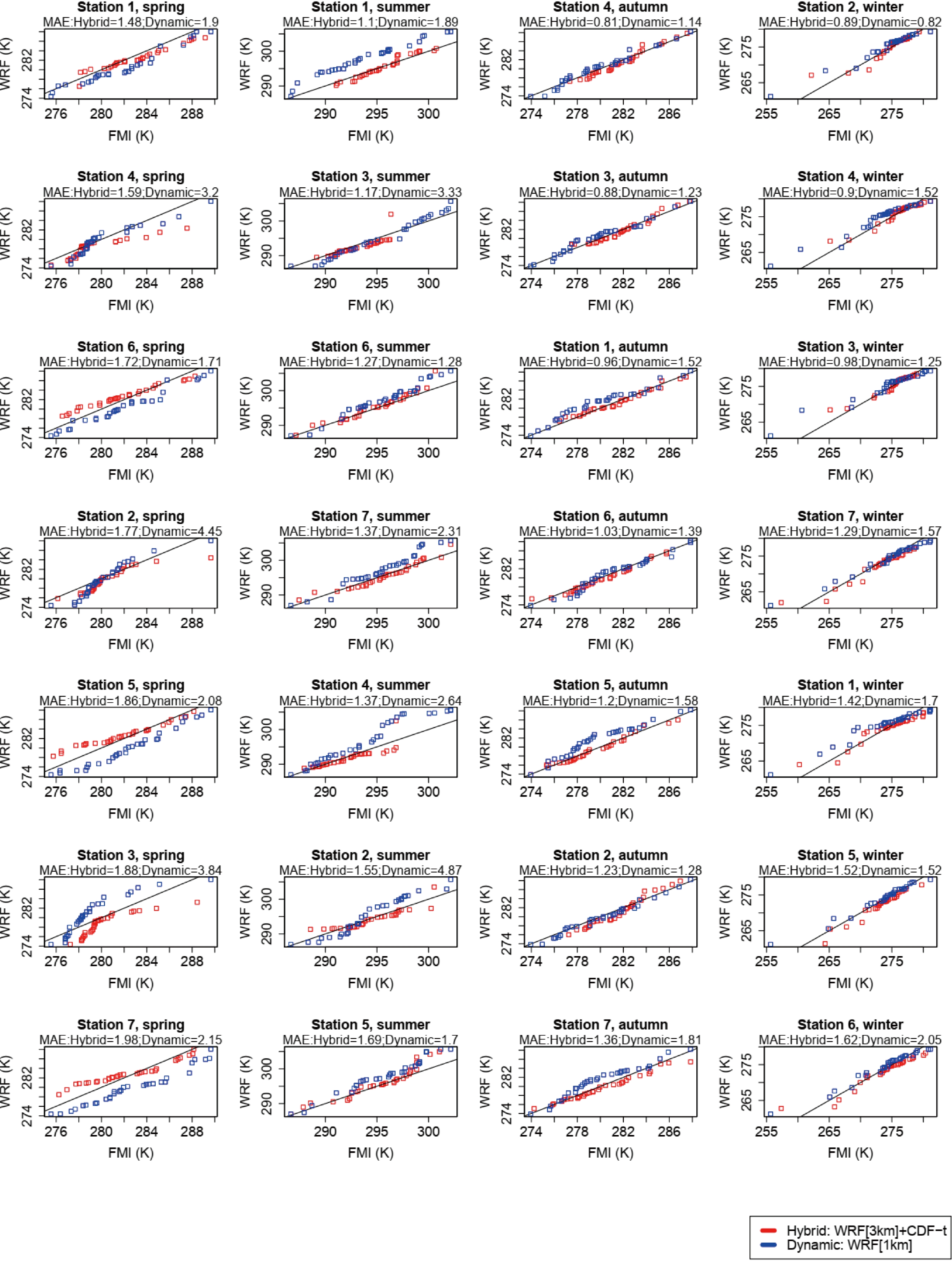 Figure4. As in Fig. 3 but for the daily maximum air temperature (K).
| Season | Method | Station | ||||||
| 1 | 2 | 3 | 4 | 5 | 6 | 7 | ||
| Spring: April 2016 | WRF[3 km]+CDF-t | 0.13 | 0.27 | 0.49 | 0.16 | 0.17 | 0.21 | 0.31 |
| WRF[1 km] | 0.73 | 3.68 | 3.28 | 2.64 | 0.50 | 0.25 | 0.37 | |
| Summer: July 2016 | WRF[3 km]+CDF-t | 0.07 | 0.16 | 0.30 | 0.10 | 0.06 | 0.04 | 0.05 |
| WRF[1 km] | 0.40 | 3.63 | 2.43 | 1.61 | 0.45 | 0.22 | 0.78 | |
| Autumn: Octorber 2016 | WRF[3 km]+CDF-t | 0.04 | 0.17 | 0.07 | 0.11 | 0.04 | 0.07 | 0.06 |
| WRF[1 km] | 0.12 | 0.25 | 0.20 | 0.15 | 0.08 | 0.11 | 0.14 | |
| Winter: January 2017 | WRF[3 km]+CDF-t | 0.14 | 0.21 | 0.10 | 0.13 | 0.16 | 0.09 | 0.09 |
| WRF[1 km] | 0.63 | 0.09 | 0.31 | 0.67 | 0.51 | 0.69 | 0.42 | |
Table2. As Table 1 but for the daily maximum air temperature.
As is the case for the daily mean temperature, the hybrid method gives the lowest MAEs for nearly all the stations and seasons, except for station 6 in spring and 2 in winter. In addition, some of the findings reached in the analysis of Fig. 3 hold for the daily maximum temperature, such as (i) warm bias in the model at the location of all stations in winter, at times with a magnitude larger than 5 K; (ii) warm bias in the inland stations (5, 6 and 7) and cold bias in the coastal stations (2, 3 and 4) in spring; (iii) smaller-magnitude biases in summer and autumn, particularly for the WRF[3 km]+CDF-t downscaling; (iv) not so skillful simulation of the extremes of the daily maximum temperature distribution (i.e., the tails of the CDF distributions).
Except for station 2 in winter, the CvM scores for the WRF[3 km]+CDF-t approach are smaller than those obtained with the WRF[1 km] downscaling. For this station, the MAE given by the hybrid approach is also higher. The CvM scores for the two methods averaged over all stations and seasons are 0.14 and 0.91, with RMSE values of 1.8 K and 2.4 K, and MAE values of 1.4 K and 2.1 K, respectively. The p-value obtained with the Wilcoxon rank-sum test with the same alternative hypothesis as for the daily mean temperature is 0.018. Hence, and as is the case for the daily mean temperature, the two distributions of CvM scores are statistically different from each other, with the hybrid approach giving more accurate predictions according to all the verification diagnostics considered. Despite the slightly higher magnitude of the RMSEs and MAEs compared to those of the daily mean temperature, the model-predicted daily maximum temperatures are generally within 2 K of those observed, in particular for the WRF[3 km]+CDF-t downscaling approach. As temperature extremes are likely to change more than the mean values in a hypothetical warmer world (e.g., Seneviratne et al., 2014), it is of interest to look into how the model performs in the warm (summer) and cold (winter) seasons separately. The averaged CvM scores for the hybrid, WRF[3 km]+CDF-t, and dynamical-only, WRF[1 km], downscaling are 0.11 and 1.36 for the summer and 0.13 and 0.47 for the winter season, respectively. The corresponding RMSE (MAE) scores for the hybrid and dynamical-only simulations are 1.8 K (1.4 K) and 2.9 K (2.6 K) for the summer, and 1.6 K (1.2 K) and 1.9 K (1.5 K) for the winter season, respectively. Hence, while WRF[3 km]+CDF-t clearly outperforms WRF[1 km] in the summer season, in winter the scores are more comparable, even though the hybrid approach still has the edge.
2
3.3. Daily minimum temperature
Figure 5 is similar to Fig. 3 and Table 3 is similar to Table 1 but for the daily minimum air temperature. For this field, and for all stations and seasons, roughly 0.6% of the total number of points are subjected to the Déqué (2007) out of bounds correction, i.e., less than one point per panel.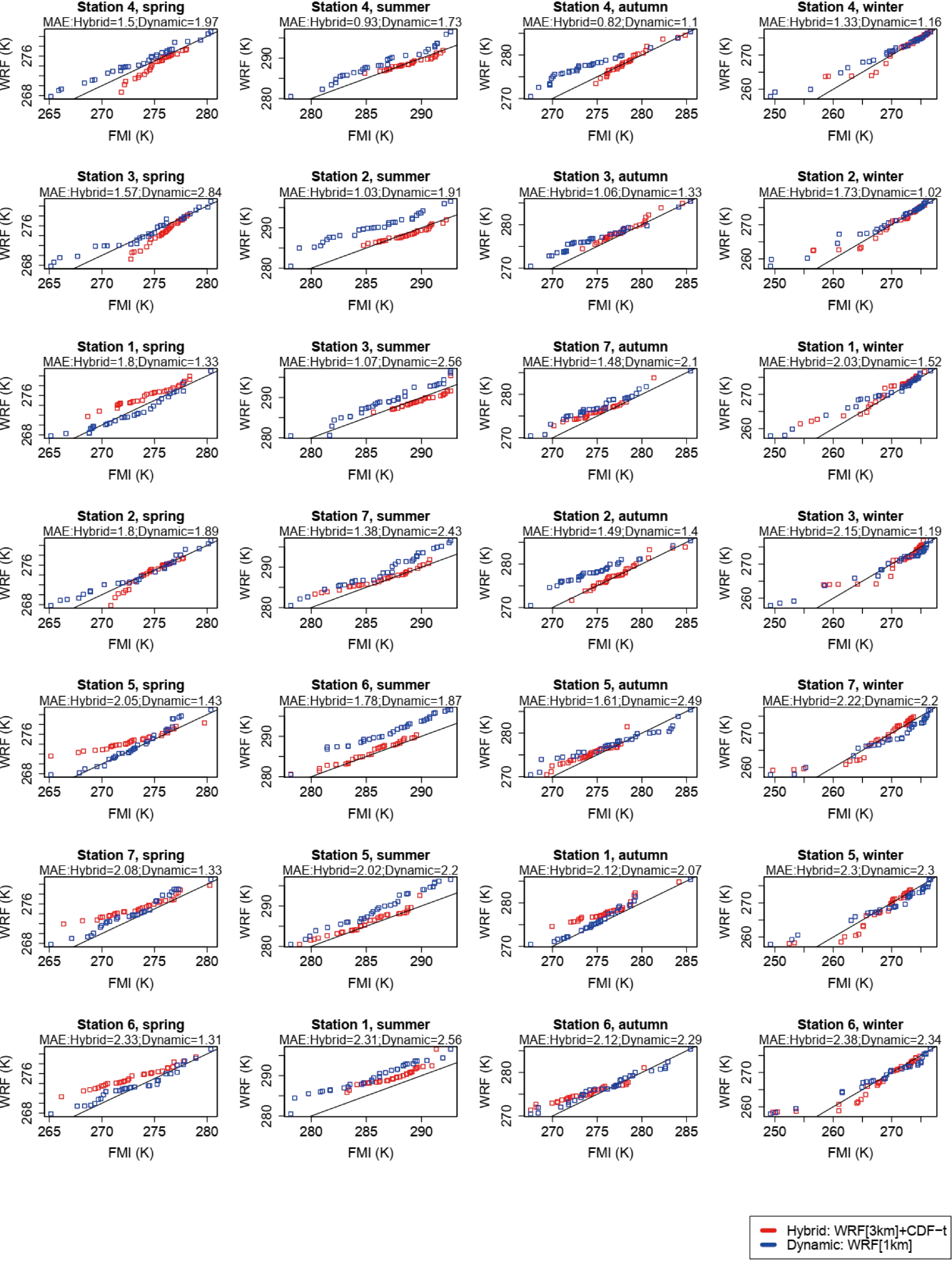 Figure5. As in Fig. 3 but for the daily minimum air temperature (K).
| Season | Method | Station | ||||||
| 1 | 2 | 3 | 4 | 5 | 6 | 7 | ||
| Spring: April 2016 | WRF[3 km]+CDF-t | 0.53 | 0.06 | 0.47 | 0.18 | 0.89 | 0.98 | 0.66 |
| WRF[1 km] | 0.24 | 1.10 | 2.44 | 1.56 | 0.25 | 0.10 | 0.18 | |
| Summer: July 2016 | WRF[3 km]+CDF-t | 1.43 | 0.12 | 0.25 | 0.07 | 0.09 | 0.08 | 0.12 |
| WRF[1 km] | 1.56 | 1.14 | 2.14 | 1.10 | 0.49 | 0.59 | 1.04 | |
| Autumn: Octorber 2016 | WRF[3 km]+CDF-t | 1.14 | 0.03 | 0.21 | 0.04 | 0.32 | 0.58 | 0.56 |
| WRF[1 km] | 0.64 | 0.05 | 0.13 | 0.04 | 0.80 | 0.10 | 0.74 | |
| Winter: January 2017 | WRF[3 km]+CDF-t | 0.18 | 0.04 | 0.08 | 0.02 | 0.05 | 0.06 | 0.10 |
| WRF[1 km] | 0.26 | 0.03 | 0.17 | 0.09 | 0.33 | 0.26 | 0.37 | |
Table3. As Table 1 but for the daily minimum air temperature.
While for the daily mean and maximum air temperatures the hybrid method clearly outperforms the dynamical-only downscaling approach, for the daily minimum air temperature the performance of the two techniques is more comparable, with generally higher MAEs. For this field, both methods show a clear warm bias not just in winter but in all seasons, even though it has a larger magnitude in the cold season. These warmer nighttime temperatures may arise from excessive cloud cover and/or deficiencies in the Noah LSM (e.g. Katragkou et al., 2015; Bastin et al., 2018). For summer and autumn, and except for stations 1 and 2 in the latter, the hybrid approach gives the lowest MAEs. In winter and spring, however, the results are mixed, even though in the former the main difference between the two methods is in the tail of the distribution. The magnitude of the MAEs is also higher for this field: while for the daily mean and maximum air temperatures the hybrid method always gives MAEs lower than 2 K, for this method and for the minimum air temperature the MAEs exceed 2 K at more than 40% of the stations. Recent work has shown that the daily minimum temperature is expected to change more significantly than the daily maximum and mean air temperatures in a hypothetical warmer world (e.g., Nikulin et al., 2011). It is possible then that the poorer performance of the hybrid method for this field may also arise from the violation of the stationary assumption made in the development of the statistical technique.
In line with the Q-Q plots shown in Fig. 5, no method is found to outperform another when inspecting the CvM scores given in Table 3. A comparison of Table 3 with Tables 1 and 2 reveals that, while for the daily mean and maximum temperatures WRF[1 km] only outperforms WRF[3 km]+CDF-t in two cases and one case, respectively, for the daily minimum temperature, the dynamical-only downscaling outperforms the hybrid approach in a total of eight cases. Looking at each season separately, four out of the eight cases occur in spring, three in autumn, and one in winter. The poorer performance of WRF[3 km]+CDF-t seems to be almost exclusively in the transition seasons. As stated before, the WRF forecasts at this time of the year, and particularly in spring, are less skillful, possibly because of deficiencies inherent to the Noah LSM that lead to discrepancies between the observed and modelled snow cover and extent of the snow season (Sheffield et al., 2003). This is confirmed when the observed and modelled snow depths are compared (not shown). The fact that the two methods give more comparable results may suggest that the CDF-t does not work so well in the transition seasons. One possible explanation is that, while in both April and October the daylight period is still relatively long, allowing for a more well-mixed atmosphere and therefore more predictable daytime temperatures, at night the better representation of the static fields and local-scale dynamics in the WRF[1 km] run may give it the edge at the location of some of the stations. Despite this, however, the p-value obtained with the Wilcoxon rank-sum test with the same alternative hypothesis as for daily mean and maximum temperatures is 0.018, indicating that at the 95% confidence level the hybrid downscaling still gives the best results. The averaged CvM scores over all stations and seasons for the hybrid and dynamical-only downscaling methods are 0.33 and 0.64, respectively. For the summer season, the scores for the WRF[3 km]+CDF-t and WRF[1 km] are 0.30 and 1.15, and for the winter season they are 0.08 and 0.22. The corresponding RMSEs (MAEs) values are 2.3 K (1.7 K) and 2.2 K (1.9 K) for all seasons, 1.8 K (1.5 K) and 2.5 K (2.2 K) for the summer season, and 2.9 K (2 K) and 2.1 K (1.7 K) for the winter season, respectively. It is interesting to note that, while for the summer season WRF[3 km]+CDF-t gives the smallest RMSE and MAE, for winter WRF[1 km] performs the best according to those two scores, even though its CvM score is higher. This apparent contradiction can be explained by looking at the Q-Q plots in Fig. 5. The main difference between the two modelled CDFs is in the tail of the distribution, with the CDF of the hybrid method showing larger discrepancies with respect to that observed. However, overall the hybrid method’s CDF is closer to the main diagonal compared to that given by the WRF[1 km] simulation, and hence it has a lower CvM but a higher RMSE and MAE. As highlighted before, the model-predicted daily minimum air temperatures forecasts are not as skillful as those for the daily mean and maximum air temperatures but are still generally within 3 K of those observed.
In the discussion so far the temperature distributions predicted by WRF[3 km]+CDF-t and WRF[1 km] are evaluated against those observed through the analysis of the correspondent Q-Q plots and the MAE and CvM scores. In order to allow for a more direct evaluation of the three temperature distributions, in Fig. 6 they are shown at the location of station 2 for the summer season. Similar results are obtained at the other stations for this season (not shown). The curves plotted in Fig. 6 are in line with the findings highlighted before: WRF[3 km]+CDF-t gives more skillful air temperature predictions compared to WRF[1 km], particularly for the daily-mean and maximum air temperatures. For these two variables, the three temperature distributions are bimodal, with the WRF[1 km] distribution exhibiting a clear cold bias, more significant for the maximum temperature. The two model-predicted distributions are more similar for the daily minimum temperature, being close to a Gaussian shape, as is the case for the observed data, which is consistent with the more comparable MAE and CvM scores given in Fig. 5 and Table 3.
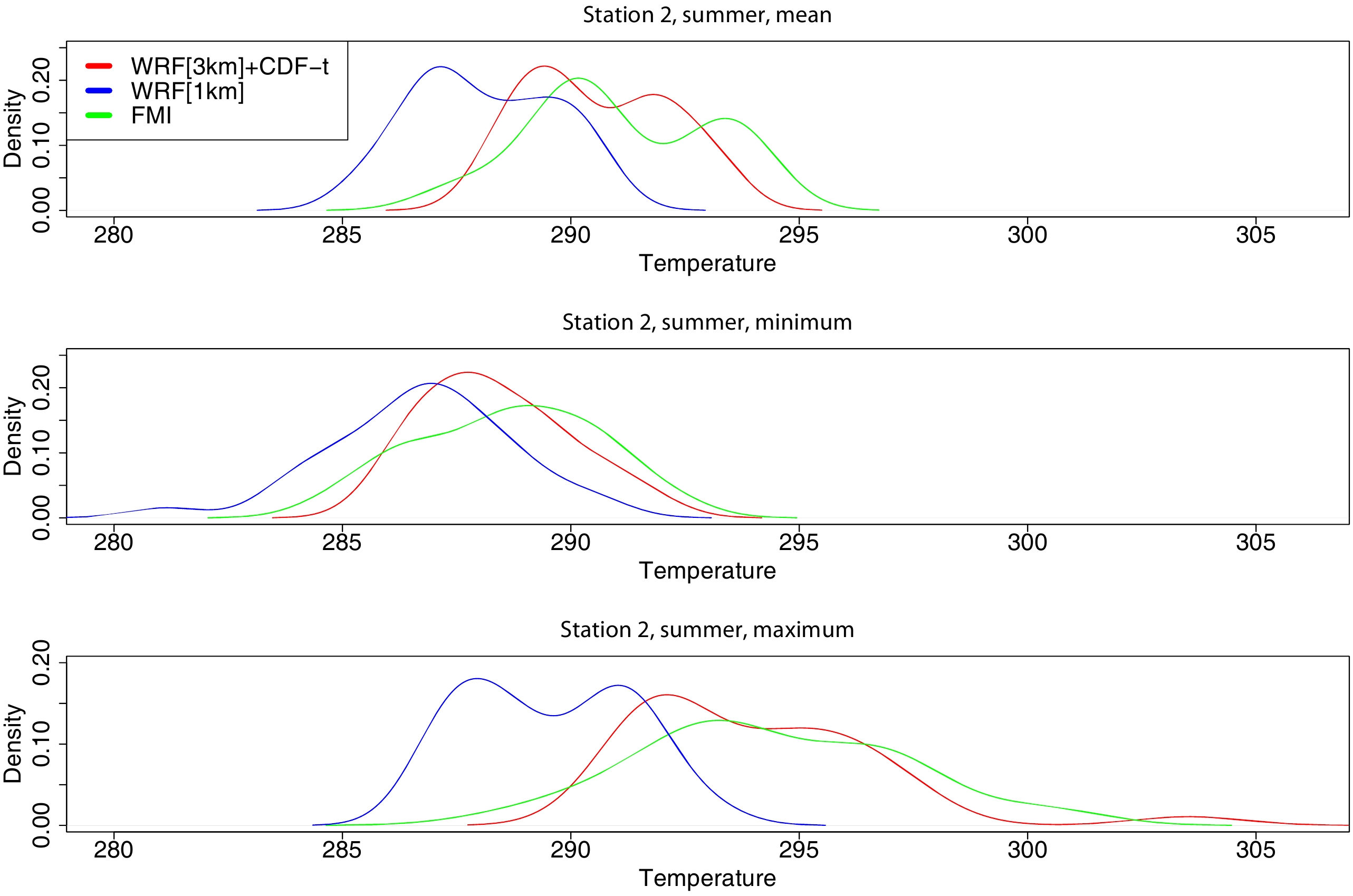 Figure6. Daily mean, minimum and maximum air temperature distributions (K) from WRF[3 km]+CDF-t (red curve), WRF[1 km] (blue curve) and that observed as given by the FMI data (green curve) at the location of station 2 and for the summer season.
For the “training” period, a 20-year (April 1997 to March 2016) WRF downscaling at a 3-km resolution, WRF[3 km], and station data from the FMI are used. A separate transformation T is generated for each season and variable, and then used to predict the daily mean and extremes of air temperature for the central month of each season for the period April 2016 to March 2017. These predictions are then compared to those given by a 1-km WRF downscaling, WRF[1 km]. The computational cost of the WRF[1 km] simulations is the reason why the prediction period is restricted to the central month of each season for one year. This is a limitation of the study, given that the atmospheric conditions in the region are known to exhibit significant variability on interannual time scales (e.g., Toniazzo and Scaife, 2006; Gray et al., 2016). A comprehensive evaluation will be presented in a subsequent paper. The performance of WRF[3 km]+CDF-t is evaluated against that given by WRF[1 km] and the FMI data both visually, through inspection of the correspondent Q-Q plots, and quantitatively, using the CvM, RMSE and MAE diagnostics. It is concluded that, at the 95% confidence level, the hybrid approach, particularly for the daily mean and maximum air temperatures, gives more skillful forecasts compared to the dynamical-only downscaling at a higher spatial resolution, at least for the near-coast Finnish region studied. For the daily minimum air temperature, however, the two methods perform comparably.
For all stations and variables, WRF has a warm bias in winter that has been noted by García-Díez et al. (2013) and is possibly due to deficiencies in the simulation of stably stratified environments, a regular occurrence at high latitudes in the cold season. In spring, on the other hand, WRF yields temperatures that are too warm at the inland stations and too cold in coastal areas. While the former may be related to the tendency of the Noah LSM to underpredict the amount of snow cover and the length of the snow season (e.g., Sheffield et al., 2003), the latter may arise from an incorrect representation of the sea-ice cover and extent, perhaps the timing of the spring melt, that are read in from the 6-hourly CFSR data. The daily minimum temperatures in WRF are too warm in all seasons, not just in winter, although the biases have a larger magnitude in the cold season. A possible explanation is excessive cloud cover and/or potential deficiencies in the Noah LSM (e.g., Katragkou et al., 2015; Bastin et al., 2018).
For the daily mean and maximum temperatures, the hybrid approach, WRF[3 km]+CDF-t, gives the best scores at nearly all stations and seasons, with averaged CvM values of about 0.15 and 0.14, RMSE values of 1.5 K and 1.8 K, and MAE values of 1.9 K and 1.4 K, respectively. On the other hand, for the daily minimum temperature, the results obtained with the two techniques are more comparable, with WRF[1 km] outperforming WRF[3 km]+CDF-t for four stations in spring, three in autumn, and one in winter. In addition to the more variable weather conditions in the transition seasons that may be harder to simulate with the CDF-t, the predicted more significant changes in the daily minimum air temperature compared to the daily maximum and mean temperatures in a future warming climate (e.g., Nikulin et al., 2011) may suggest that the stationary assumption made in the CDF-t technique does not work so well for this field. In any case, and for the hybrid approach, the CvM score for the daily minimum temperature is about 0.33, the RMSE is 2.3 K, and the MAE is 1.7 K. These scores show an overall good performance and highlight the potential use of this WRF product for in-situ air temperature estimation, at least for this region. These results are confirmed by a direct inspection of the observed, WRF[3 km]+CDF-t and WRF[1 km] air temperature distributions.
As the CDF-t does not require much time and computational resource to implement, this methodology can easily be extended to other variables (e.g., precipitation, and quantities related to wind energy and icing applications), regions, numerical models and future climate change studies. Some of the referred extensions of the work will be presented in a subsequent paper. Future work will also test better treatments of the tail adjustment of the modelled CDF, such as the one proposed by Lanzante et al. (2019).
Acknowledgements. We acknowledge Botnia-Atlantica, an EU-programme financing cross border cooperation projects in Sweden, Finland and Norway, for their support of this work through the WindCoE project. We would like to thank the High Performance Computing Center North for providing the computer resources needed to perform the numerical experiments presented in this paper. We would like to thank the three anonymous reviewers for their detailed and insightful comments and suggestions, which helped to improve the quality of the paper.
