Hang Xu¹, Qiang Sun^{,2,?? 1} State Key Laboratory of Ocean Engineering, School of Naval Architecture, Ocean and Civil Engineering, Shanghai Jiao Tong University, Shanghai 200240, China
² Particulate Fluids Processing Centre, Department of Chemical Engineering, The University of Melbourne, Parkville, VIC 3010, Australia

Corresponding authors: ?qiang.sun@unimelb.edu.au

Received:2019-02-14Online:2019-08-1

Fund supported:

* Supported by the National Natural Science Foundation of China under Grant .Nos. 118722 the National Natural Science Foundation of China under Grant .11432009 and the Australian Research Council through a Discovery Early Career Researcher Award .DE150100169

Abstract
The fully developed mixed convection hybrid nanofluid flow in a vertical microchannel is examined in detail. The simplified hybrid model that omits the nonlinear terms due to the interaction of different nanoparticle volumetric fractions is derived and compared with the existing one. The generalized model describing hybrid nanofluid suspended with multiple kinds of solid particles is suggested. The argument that the corresponding nanofluid solutions obtained by the homogenous model can be recovered from the results of the regular problems through simple arithmetic operations is checked. Solutions in similarity form for this flow problem are formulated by means of a set of similarity variables. The effects of various parameters on important physical quantities are analyzed and discussed.
Keywords： hybrid nanofluid;vertical channel;mixed convection;slippery effect


PDF (857KB)MetadataMetricsRelated articlesExportEndNote|Ris|BibtexFavorite
Cite this article
Hang Xu, Qiang Sun. Generalized Hybrid Nanofluid Model with the Application of Fully Developed Mixed Convection Flow in a Vertical Microchannel ^*. [J], 2019, 71(8): 903-911 doi:10.1088/0253-6102/71/8/903

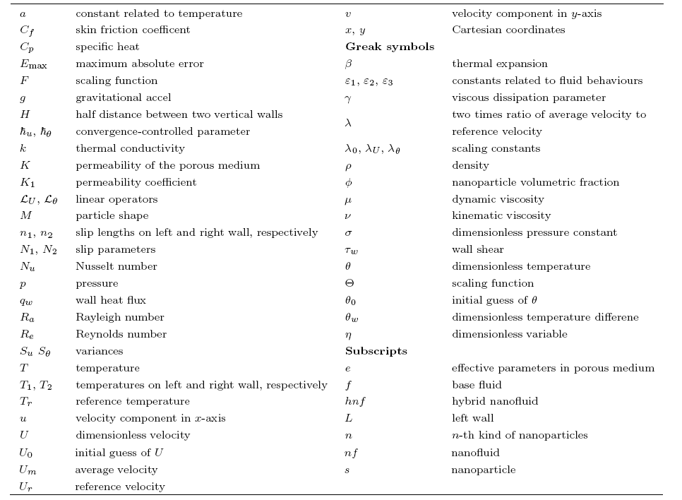
Nomenclature

1 Introduction

Many recent studies revealed that nanofluids have better heat transfer capability than regular fluids. Therefore it is possible to replace traditional heat transfer fluids by nanofluids in the design of various heat transfer systems such as cooling systems, heat regenerators, and heat exchangers. Choi^[1] noticed that, by suspending nanometer-sized metallic particles in conventional heat transfer fluids, the resulting nanofluids hold higher thermal conductivities than those of currently used ones. Xuan and Li^[2] attributed the heat transfer enhancement of nanofluids to the increase of thermal conductivity of the nanofluid. Eastman et al.^[3] found that the particle shape has stronger effects on effective nanofluid thermal conductivity than particle size or particle thermal conductivity. Wen and Ding^[4] speculated that possible reasons for the heat transfer enhancement of nanofluids are due to the migration of nanoparticles and the resulting disturbance of the boundary layer. Buongiorno^[5] concluded that the Brownian diffusion and thermophoresis are dominant factors for heat enhancement within the boundary layer owing to the effect of the temperature gradient and thermophoresis. Other classic researches on nanofluids have been experimentally done by Pak and Cho,^[6] Xie et al.,^[7] Williams et al.^[8] and numerically done by Tiwari and Das,^[9] Oztop and Abu-Nada,^[10] Raza et al.,^[11] Khan,^[12] Sajid et al.,^[13] Sheikholeslami and Sadoughi,^[14] Sheremet and Pop,^[15] Kefayati^[16] and Alsabery et al.^[17]

Some researchers made attempts to investigate the characters of nanofluids containing different kinds of nanoparticles. Suresh et al.^[18] found that both thermal conductivity and viscosity of hybrid nanofluids increase with the nanoparticle volume concentration while the viscosity increase is substantially higher than the increase in thermal conductivity for an Al$_2$O$_3$-Cu hybrid nanofluid. The behaviours of hybrid nanofluids then were examined in detail by different researchers such as Esfe et al.,^[19] Rostamian et al.^[20] and Ebrahimi and Saghravani.^[21] From modelling point of view, Devi and Devi^[22] proposed a mathematical model to investigate the effects of Lorentz force over a three-dimensional stretching surface subject to Newtonian heating. Tayebi and Chamkha^[23-24] considered natural convection in an annulus between two confocal elliptic cylinders and eccentric horizontal cylinders filled with a Cu-Al$_2$O$_3$/water hybrid nanofluid.

Huminic and Huminic^[25] examined the influence of hybrid nanofluids on the performances of elliptical tube. Rostami et al.^[26] considered mixed convective stagnation-point flow of an aqueous silica Calumina hybrid nanofluid.

This paper intends to analyze a fully developed mixed convection hybrid nanofluid flow in a vertical microchannel by means of a generalized hybrid nanofluid model. We are to simplify the Devi and Devi's model^[22] by omitting the nonlinear terms due to the interaction of different nanoparticle volumetric fractions. Then we extend Devi and Devi's model^[22] to the case that the hybrid nanofluids contain various kinds of nanoparticles. The argument by Magayari^[27] that corresponding nanofluid results can be recovered from the solutions of already solved regular problems by simple arithmetic operations is then checked. The similarity solutions for this microchannel flow and heat transfer of a hybrid nanofluid are formulated by means of a set of similarity variables. It should be on hybrid nanofluids are still very new at this stage. There is no conclusive idea on how nanoparticles act on fluid flow and heat transfer. Complementary studies are urgently needed to understand the heat transfer characteristics of hybrid nanofluids, especially for those in suspension of multiple kinds of small particles.

2 Generalized Hybrid Nanofluid Model

In experimental and numerical studies on nanofluids' behaviours, it is a common practice to model their physical quantities by using simplified mathematical relations between the corresponding ones of base fluid and solid particles, as presented by many researchers such as Vajravelu et al. and^[28] Devi and Devi.^[22] Several experiments have been carried out to confirm the validity of such expressions for dilute nanofluids in suspension of one single kind of solid particles^[6] and two types of mixed solid particles.^[18] Devi and Devi^[22] suggested a group of correlations for physical quantities of hybrid nanofluids. In their approach, they took the fluid containing one kind of nanoparitcles as the base fluid and the other kind of nanoparticles as the individual particles. The correlations of viscosity and thermal conductivity matched the experimental results given by Suresh et al.^[18]

In Devi and Devi's approach,^[22] there are nonlinear terms due to the interaction of two kinds of different nanoparticles. However, in dilute solutions in which the nanoparticle volumetric fractions are usually small, the effects of these nonlinear terms may not be significant. Therefore, we reasonably neglect the nonlinear terms in Devi and Devi's model.^[22] Our simplified model of hybrid nanofluid, as well as the classic nanofluid model and Devi and Devi's model^[22] are listed in Table 1 in which Type I denotes the traditional nanofluid model (nanofluid in suspension one kind of small particles), Types II and III, respectively, denote Devi and Devi's hybrid nanofluid model^[22] and our simplified hybrid nanofluid model (nanofluid in suspension two different kind of small particles).


Table 1
Table 1Models of nanofluid and hybrid nanofluid

New window|CSV

Devi and Devi's approach^[22] used the recurrence formulae to represent the viscosity, density, specific heat and thermal conductivity of the hybrid nanofluid corresponding to the $n$-th kindsof nanoparticles as

(1) $$\rho_{hnf}\equiv\rho_{hnf_n}=(1-\phi_{n})\rho_{_{hnf_{n-1}}}+\phi_{n} \rho_{s_n}\,, $$
(2) $$(\rho c_{p})_{hnf}\equiv (\rho c_{p})_{hnf_n} \quad =(1-\phi_{n})(\rho c_{p})_{hnf_{n-1}}+\phi_{n} (\rho c_{p})_{s_n}\,,$$
(3) $$\mu_{hnf}\equiv \mu_{hnf_n}=\frac{\mu_{hnf_{n-1}}}{(1-\phi_{n})^{2.5}}\,,$$
(4) $$\beta_{hnf}\equiv\beta_{hnf_n}=(1-\phi_{n})\beta_{_{hnf_{n-1}}}+\phi_{n} \beta_{s_n}\,,$$
and

(5) $$k_{hnf}\equiv k_{hnf_n} =\frac{k_{s_n}+(M-1) k_{hnf_{n-1}}-(M-1)\phi_{n}(k_{hnf_{n-1}}-k_{s_n})}{k_{s_n}+(M-1)k_{hnf_{ n-1}}+\phi_{n}(k_{hnf_{n-1}}-k_{s_n})}k_{hnf_{n-1}}\,. $$
By neglecting the nonlinear terms in above correlations, we obtain

(6) $$\rho_{hnf}=1- \rho_{f} \sum_{j=1}^n \phi_{j}+ \sum_{j=1}^{n} \phi_{j}\rho_{s_{j}},$$
(7) $$(\rho c_{p})_{hnf} =1-(\rho_f C_p)_f \sum_{j=1}^n \phi_{j}+\sum_{j=1}^n \phi_{j}(\rho C_p)_{s_j},$$
(8) $$\mu_{hnf}=\frac{\mu_f}{(1-\sum\limits_{j=1}^n \phi_{j})^{2.5}},$$
(9) $$\beta_{hnf}=1-\beta_f \sum_{j=1}^n \phi_{j}+\sum_{j=1}^n \phi_{j}\beta_{s_j}.$$
Note that we keep the recurrence formula (5) for the thermal conductivity $k_{hnf}$ since the interactions between different particles can hardly be expressed using the Maxwell equation. Also, $M=3$ is chosen throughout this work that means that the particle shape is spherical.

3 Mathematical Description

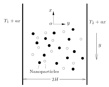
Consider a mixed convection flow of a hybrid nanofluid in a constant porosity medium between two parallel vertical infinite walls separated by a distance of $2H$. As shown in Fig. 1, the Cartesian coordinate system ($x, y$) is chosen with the $x$-axis being along the walls and the $y$-axis being perpendicular to the walls. The temperatures on both walls are assumed to vary linearly along the height that are prescribed as $T_1+a x$ and $T_2+a x$ on the left and the right walls, respectively. Since the hydrodynamically flow is fully-developed, the velocity along the wall is only a function of $y$. Invoking the Boussinesq approximation, the governing equations are written as

(10) $$\frac{\partial u}{\partial x}+\frac{\partial v}{\partial y}=0\,,$$
(11) $$\frac{\partial p}{\partial x}=\mu_{ehnf}\frac{\partial^2 u}{\partial y^2}-\frac{\mu_{hnf}}{K} u+(\rho \beta)_{hnf}g(T-T_r)\,,$$
(12) $$\frac{\partial p}{\partial y}=0\,,$$
(13) $$u\frac{\partial T}{\partial x}+ v \frac{\partial T}{\partial y}=\alpha_{ehnf} \Big(\frac{\partial^{2}T}{\partial x^{2}}+ \frac{\partial^{2}T}{\partial y^{2}} \Big) +\frac{\mu_{hnf}}{K (\rho C_{_p})_{hnf}} u^2\,,$$
subject to the boundary conditions

(14) $$u=n_2 \frac{\partial u}{\partial y}\,, \quad T=T_2+a x\,, \quad {\rm at}\quad y= H\,,$$
(15) $$u=n_1 \frac{\partial u}{\partial y}\,, \quad T=T_1+a x\,, \quad {\rm at}\quad y= -H\,.$$

Fig. 1

New window|Download| PPT slide
Fig. 1Physical sketch.



It is easy to see from Eq. (12) that ${\partial^2 p}/{\partial x \partial y}=0$. This indicates that ${\partial p}/{\partial x}$ is a constant and that all terms on the right-hand side of Eq. (11) are only dependent on $y$. Based on this fact, we define the following variables

(16) $$\eta=\frac{y}{H}\,, \quad U(\eta)=\frac{u}{U_{_r}}\,,\quad \theta(\eta)=\frac{T-T_{_r}}{a H}\,,$$
where $U_{r}=g \beta_{f} K a H/{\nu_{f}}$ is a reference velocity.

Substituting Eq. (16) into Eqs. (10), (11), and (13), the continuity equation (10) is automatically satisfied, and the rest of equations are reduced to

(17) $$U^{\prime\prime}+K_{1}(\varepsilon_1 \theta- U)+\sigma=0\,,$$
(18) $$\theta^{\prime\prime}-\varepsilon_{2} R_{a}U + \varepsilon_{3} \gamma R_{a} U^2=0\,,$$
with the boundary conditions

(19) $$U(1)=N_2 U'(1)\,, \quad U(-1)=N_1 U'(-1)\,, \theta(1)=\theta_w\,, \quad \theta(-1)=-\theta_w \,,$$
where

(20)$$\varepsilon_1=\Big(\frac{\beta_{hnf}}{\beta_{f}}\Big)\Big(\frac{\mu_{f}}{\mu_{hnf}}\Big)\Big(\frac{\rho_{hnf}}{\rho_{f}}\Big)\,, \\ \varepsilon_2=\frac{k_{ef}}{k_{ehnf}} \frac{(\rho C_{_p})_{hnf}}{(\rho C_{_p})_{f}}\,, \quad \varepsilon_3 = \frac{\mu_{nhf}}{\mu_f}\frac{k_{ef}}{k_{enhf}}\,, \\ K_{1}=\frac{\mu_{hnf}}{\mu_{ehnf}}\frac{H^2}{K}\,, \quad R_{a}=\frac{g \beta_f K a H^2}{\alpha_f\nu_f}\,,\\ \gamma=\frac{g \beta_{f} H}{C_{pf}}\,, \quad \sigma=-\frac{H^2}{\mu_{hnf} U_r}\frac{\partial p}{\partial x}\,,\\ \theta_w=\frac{T_2-T_1}{2 a H}\,, \quad N_1=\frac{n_1}{H}\,, \quad N_2=\frac{n_2}{H}\,. $$

4 Comparison Analysis Between Models

We calculate the coefficients $\varepsilon_1$, $\varepsilon_2$, and $\varepsilon_3$ in Eqs. (17) and (18) by Type II and Type III hybrid nanofluid models listed in Table 1. The data regarding to the basic thermo-physical properties of the base fluid and nanoparticles are given in Table 2 where the thermophysical properties of water is chosen at 25$^{C}$.


Table 2
Table 2Thermophysical properties of fluid and nanoparticles.

New window|CSV

Substituting the quantities in Table 2 into different hybrid nanofluid models, the values of $\varepsilon_1$, $\varepsilon_2$, and $\varepsilon_3$ can be obtained, as shown in Table 3. It can be seen from the table, when the solution is dilute, namely, the nanoparticle volumetric fractions are small, the difference between the values of $\varepsilon_1$, $\varepsilon_2$ and $\varepsilon_3$ obtained by both models is imperceptible. Recalling the experimental results and modelling tests by Pak et al.^[6] and Suresh et al.,^[18] it is clear that the computational range of nanoparticle volumetric fractions listed in Table 3 is acceptable and widely used. As a result, we can infer that our simplified hybrid nanofluid model is meaningful for prediction of nanofluids' behaviours. Further verification shows that, for the cases that two kinds of nanoparticles coexist, each nanoparticle volumetric fraction needs to be small to keep the solution remaining dilute.


Table 3
Table 3Computation of nanoparticles related parameters.*
* Note: Here the nanoparticles are Al2O3 and Cu, respectively.

New window|CSV

Magyari^[27] once found that, without consideration of velocity-slip effects, the governing equations of homogeneous nanofluid models can be reduced via elementary scaling transformations to the corresponding equations of the regular fluids. Thus he concluded that the corresponding nanofluid results can be recovered from the solutions of already solved problems with regular Newtonian fluids by simple arithmetic operations.

Here, we would like to check if this applicability is valid on the hybrid nanofluid flow problems. We introduce the following scaling transformations:

(21) $$U(\eta)=\lambda_U F(\xi)\,, \quad \theta = \lambda_\theta \Theta(\xi)\,, \quad \eta=\lambda_0 \xi\,.$$
Substituting Eq. (21) into Eqs. (17) and (18), we obtain

(22)$$ \frac{\lambda_U}{\lambda_0^2}F^{\prime\prime}+K_1(\epsilon_1 \lambda_\theta \Theta - \lambda_U F)+\sigma=0\,,$$
(23) $$\frac{\lambda_\theta}{\lambda_0^2}\Theta^{\prime\prime}-\epsilon_2 R_a \lambda_U F+\epsilon_3 \gamma R_a \lambda_U^2 F^2=0\,.$$
To keep Eqs. (22) and (23) invariant in forms, the two relationships below must hold:

(24) $$\frac{\lambda_U}{\lambda_0^2}= \lambda_\theta=\lambda_U\,,$$
(25) $$\frac{\lambda_\theta}{\lambda_0^2}=\lambda_U=\lambda_U^2\,,$$
which leads to

(26) $$\lambda_\theta=\lambda_U=\lambda_0 \equiv 1\,.$$
Equation (26) clearly indicates that, for the problem considered in this work, there is no alternative scaling transformation that can be used to obtain solutions from the existing results. We therefore are able to conclude that Mayari's conclusion^[27] on that nanofluid results can be recovered from the solutions of already solved regular Newtonian fluid problems by simple arithmetic operations is only valid for several special cases in nanofluid researches.

5 Results

It is known that Eq. (17) contains an unknown constant $\sigma$, which requires an additional boundary condition. In the studies on channel flow problems, it is a common practice to sprecify the mass flow rate as a prescribed quantity. We thus obtain

(27) $$U_m=\frac{1}{2 H}\int_{-H}^{H} ud y\,,$$
which can be simplified, by using the similarity variables (16), to

(28) $$\int_{-1}^{1} Ud \eta =\lambda\,,$$
where $U_m$ is the constant average flow velocity across the channel, and $\lambda=2{U_m}/{U_r}$. For convenience, we let $U_m=U_r$ which leads to $\lambda=2$.

The homotopy analysis method (HAM) is used to solve this flow problem. Since the similar HAM procedures are available in Refs. [29-30], we omit the detailed process but just give the core information as shown in Table 4.


Table 4
Table 4HAM computation related quantities.

New window|CSV

To check the accuracy of our solutions, we define the following functions to evaluate errors:

(29) $$E_{\max}=\max(S_u^{1/2},S_\theta^{1/2})\,,$$
where

(30) $$S_u=\int_{-1}^1 [U^{\prime\prime}+K_{1}(\varepsilon_1 \theta- U)+\sigma]^2 d\eta\,,$$
(31) $$S_\theta =\int_{-1}^1 [\theta^{\prime\prime}-\varepsilon_{2} R_{a}\, U + \varepsilon_{3} \gamma R_{a} U^2]^2 d\eta\,.$$
When all physical parameters are prescribed, the corresponding errors can be obtained. For example, if we set $R_a=10$, $\gamma=1/100$, $K_1=1$, $N_1=1/10$, $N_2=-1/10$, and $\theta_w=1/10$, and prescribe $\phi_1$ and $\phi_2$ for a range of values, at a certain HAM computational order, the errors can be determined by Eq. (29) as shown in Table 5.


Table 5
Table 5Absolute errors for various values of $\phi_1$ and $\phi_2$ at 40-th HAM computational order.

New window|CSV

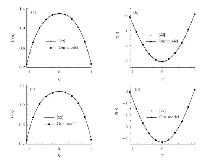
Further to check the validity and accuracy of our simplified model, we compare our results of velocity and temperature profiles for a hybrid nanofluid in suspension of two types of nanoparticles with those given by Devi and Devi.^[22] It can be seen in Figs. 2(a) and 2(b) that very good agreement is found. Note that here Al$_2$O$_3$ and Cu nanoparticles are chosen for comparison. As shown in Figs. 2(a) and 2(b), we also notice that the results by our simplified hybrid nanofluid model match to those given by the generalized hybrid nanofluid model when three types of nanoparticles, namely, Al$_2$O$_3$, Cu and TiO$_2$ are employed.

Fig. 2

New window|Download| PPT slide
Fig. 2Comparisons of $U(\eta)$ and $\theta(\eta)$ in the case of $R_a=10$, $\gamma=1/100$, $K_1=1$, $N_1=1/10$, $N_2=-1/10$, $\theta_w=1/10$. Line with gradients: solutions by Devi and Devi's model,^[22] Line with circles: solutions by our model. (a) $\phi_1=\phi_2=1/10$. (b) $\phi_1=\phi_2=1/10$. (c) $\phi_1=\phi_2=\phi_3=3/100$. (d) $\phi_1=\phi_2=\phi_3=3/100$.


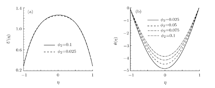
In our computation, it is found that the variation of nanoparticle volumetric fraction plays limited influence on velocity profiles while it has significant effect on the temperature profiles, as shown in Fig. 3. This indicates that the increase of nanoparticle volumetric fraction can enhance heat transfer significantly. In another words, this also verifies the fact that the nanofluids have better thermal transport capability than traditional ones.

Fig. 3

New window|Download| PPT slide
Fig. 3Variation of (a) $U(\eta)$ and (b) $\theta(\eta)$ with $\phi_2$ for $R_a=10$, $\gamma=1/100$, $K_1=1$, $N_1=1/10$, $N_2=-1/10$, $\theta_w=1/10$, $\phi_1=25/1000$.



Physically, the skin friction and the Nusselt number are important quantities to measure the fluid behaviours. Since the flow and heat transfer exhibit similar characters on both walls, we therefore only consider those quantities on the left wall. In this situation, they are defined by

(32) $$C_{fL}=\frac{\tau_{wL}}{\rho_{hnf}U_m^2}\,, \quad N_{uL}=\frac{q_{wL}L}{k_{hnf}(T_1-T_r)}\,,$$
where

(33) $${\tau_{wL}}=\mu_{hnf} \Big(\frac{\partial u}{\partial y}\Big)_{y=-H}, \quad q_{wL}=-k_{hnf} \Big(\frac{\partial T}{\partial y}\Big)_{y=-H}. $$
Substituting similarity variables in Eq. (16) into Eq. (32), we obtain

(34) $$C_{fL}=\frac{1}{Re}U'(-1)\,, \quad N_{uL}=\frac{2a}{T_2-T_1} \theta'(-1)\,,$$
where $Re=U_mH/\nu_{nhf}$ is the Reynolds number.

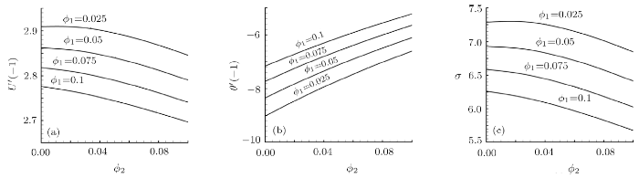
To test the effects of the nanoparticle volumetric fractions $\phi_1$ and $\phi_2$ on various physical quantities, we select Al$_2$O$_3$ and Cu nanoparticles in following analysis. As shown in Fig. 4(a), for a certain value of $\phi_1$, the absolute value of the skin friction coefficient $C_{fL}$ reduces as $\phi_2$ enlarges. Similarly, when $\phi_2$ is prescribed, the absolute value of $C_{fL}$ decreases as $\phi_1$ evolves. This clearly shows that the nanofluids can effectively diminish the skin friction. The slip effects between the velocities of nanoparticles and the base fluid is the key factor to affect the Nusselt number. The trend of $N_{uL}$ varies with $\phi_2$ is similar to that of $C_{fL}$, namely, when $\phi_1$ is given, the increase of $\phi_2$ causes the decrease of the absolute value of $N_{uL}$, or verse visa, as shown in Fig. 4(b). As concluded by Buongiorno,^[5] the temperature difference between the walls and the fluid can alter the temperature gradient and thermophoresis, which could result in a significant decrease of viscosity within the boundary layer, thus leading to heat transfer enhancement.

Fig. 4

New window|Download| PPT slide
Fig. 4Variation of (a) reduced $C_{fL}$, (b) reduced $N_{uL}$ and (c) $\sigma$ with $\phi_2$ for some values of $\phi_1$ in the case of $R_a=10$, $\gamma=1/100$, $K_1=1$, $N_1=1/10$, $N_2=-1/10$, $\theta_w=1/10$.



The effect of nanoparticle volumetric fractions on the pressure constant is shown in Fig. 4(c). For a given value of $\phi_1$, it is found that the pressure decreases gradually as $\phi_2$ grows. Same trend is found for the variation of the pressure constant $\sigma$ with $\phi_1$ at a fixed value of $\phi_2$. This reflects another aspect that the flow velocity reduces owing to the reduction of skin friction caused by the increase of nanoparticle volumetric fractions, either for nanofluids or hybrid nanofluids.

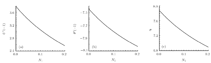
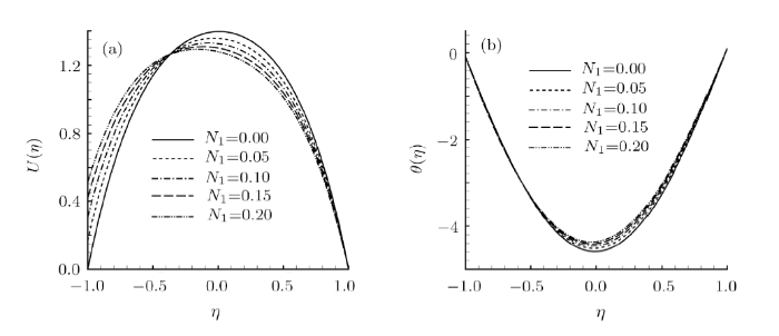
In microchannel studies, the slip of the channel wall is of great importance to alter flow and heat transfer behaviours. Take the hybrid nanofluid containing Al$_2$O$_3$, Cu and TiO$_2$ nanopaticles as an example. As shown in Fig. 5(a), the absolute value of the skin friction coefficient $C_{fL}$ decreases monotonously as $N_1$ grows. However, the absolute value of the Nusselt number $N_{uL}$ increases continuously as $N_1$ increases, as shown in Fig. 5(b), while the pressure constant $\sigma$ reduces gradually as $N_1$ enlarges, as shown in Fig. 5(c). It is seen from Fig. 6(a) that the increase of $N_1$ leads to the increase of the velocity near the left wall. This velocity variation leads to the enhancement of temperature in the channel, as presented in Fig. 6(b). Physically, the increase of the slip length indicates the decrease of the skin friction, which leads to the increase of flow velocity near that wall. Nevertheless, due to the conservation of flow flux, the flow velocity far from the left wall decreases with $N_1$ increasing.

Fig. 5

New window|Download| PPT slide
Fig. 5Variation of (a) reduced $C_{fL}$, (b) reduced $N_{uL}$ and (c) $\sigma$ with $N_1$ in the case of $R_a=10$, $\gamma=1/100$, $K_1=1$, $N_2=0$, $\theta_w=1/10$, and $\phi_1=\phi_2=\phi_3=3/100$.

Fig. 6

New window|Download| PPT slide
Fig. 6Variation of (a) $U(\eta)$ and (b) $\theta(\eta)$ with $N_1$ in the case of $R_a=10$, $\gamma=1/100$, $K_1=1$, $N_2=0$, $\theta_w=1/10$, and $\phi_1=\phi_2=\phi_3=3/100$.

6 Conclusion

The generalized hybrid nanofluid model and its simplified form have been proposed to study the flow and heat transfer behaviours of a hybrid nanofluid convection in a vertical microchannel. It has been found that when the solution is dilute, our simplified model can well predict the flow and heat transfer behaviours of hybrid nanofluids. The argument by Magyari^[27] with regards to the homogenous model for expressions of nanofluid solutions by the results of already solved regular Newtonian fluid problems via simple arithmetic operations has been found problematic when it is applied to hybrid nanofluid flows. The effects of various parameters on important physical quantities are analysed and discussed with the following conclusions can be reached:

(i) The variations of nanoparticle volumetric fractions have more obvious effects on temperature distribution than on velocity distribution.

(ii) The nanoparticle volumetric fractions play a significant role on altering flow and heat transfer behaviours.

(iii) The slip effect of the channel wall are of great importance to affect the flow and heat transfer behaviours.

Reference View Option By original order
By published year
By cited within times
By Impact factor

[1] S. Choi, in Proceedings of the 1995 ASME International Mechanical Engineering Congress and Exposition FED 231/MD66, ASME, San Francisco, CA, USA (1995).
[Cited within: 1]

[2] Y. Xuan and Q. Li, Int. J. Heat Fluid Flow 21 (2000) 58.
[Cited within: 1]

[3] J. Eastman, S. Choi, S. Li, et al. , Appl.Phys. Lett. 78(2001) 718.
[Cited within: 1]

[4] D. Wen and Y. Ding, Int. J. Heat Mass Transfer 47 (2004) 5181.
[Cited within: 1]

[5] J. Buongiorno, J. Heat Transf. Trans. ASME 128 (2006) 240.
[Cited within: 2]

[6] B. C. Pak and Y. Cho, Exp. Heat Transfe 11 (1998) 151.
[Cited within: 3]

[7] H. Q. Xie, H. Lee, W. Youn, M. Choi, J. Appl. Phys. 94(2003) 4967.
[Cited within: 1]

[8] W. Williams, J. Buongiorno, L. Hu, J. Heat Transfer Trans. ASME 130 (2008) 042412

[Cited within: 1]

[9] R. Tiwari and M. K. Das, Int. J. Heat Mass Transfer 50 (2007) 2002.
[Cited within: 1]

[10] H. Oztop and E. Abu-Nada, Int. J. Heat Fluid Flow 29 (2008) 1326.
[Cited within: 1]

[11] J. Raza, A. Rohni, Z. Omar, Int. J. Heat Mass Transfer 103 (2016) 336.
[Cited within: 1]

[12] I. Khan, J. Mol. Liq. 233(2017) 442.
[Cited within: 1]

[13] M. Sajid, S. A. Iqbal, M. Naveed, Z. Abbas, J. Mol. Liq. 233(2017) 115.
[Cited within: 1]

[14] M. Sheikholeslami and M. K. Sadoughi, Int. J. Heat Mass Transfer 116 (2018) 909.
[Cited within: 1]

[15] M. Sheremet, I. Pop, A. shenoy, Int. Commun. Heat Mass Transfer 67 (2015) 66.
[Cited within: 1]

[16] G. H. R. Kefayati, Int. J. Heat Mass Transfer 108 (2017) 1481.
[Cited within: 1]

[17] A. I. Alsabery, M. A. Ismael, A. J. Chamkha, I. Hashim, Int. J. Heat Mass Transfer 119 (2018) 939.
[Cited within: 1]

[18] S. Suresh, K. P. Venkitaraj, P. Selvakumar, M. Chandrasekar, Colloid Surface A Physicochem. Eng.Asp. 388(2011) 41.
[Cited within: 4]

[19] M. H. Esfe, S. Wongwises, A. Naderi, et al., Int. Commun. Heat Mass Transfer 66 (2015) 100.
[Cited within: 1]

[20] S. H. Rostamian, M. Biglari, S. S. Saedodin, M. H. Esfe, J. Mol. Liq. 231(2017) 364.
[Cited within: 1]

[21] S. Ebrahimi and S. F. Saghravani, Heat Mass Transfer 54 (2018) 999.
[Cited within: 1]

[22] S. S. U. Devi and S. A.Devi, Can. J. Phys. 94(2016) 490.
[Cited within: 12]

[23] T. Tayebi and A. J. Chamkha, Numer. Heat Transfer A 70 (2016) 1141.
[Cited within: 1]

[24] T. Tayebi and A. J. Chamkha, Numer. Heat Transfer A 71 (2017) 1159.
[Cited within: 1]

[25] G. Huminic and A. Huminic, Int. J. Heat Mass Transfer 129 (2019) 132.
[Cited within: 1]

[26] M. N. Rostami, S. Dinarvand, I. Pop, Chin. J. Phys. 56(2018) 2465.
[Cited within: 1]

[27] E. Magyari, ACTA Mech. 222(2011) 381.
[Cited within: 4]

[28] K. Vajravelu, K. V. Prasad, J. Lee, et al. , Int.J. Thermal Sci. 50(2011) 843.
[Cited within: 1]

[29] H. Xu and J. F. Cui, Int. J. Heat Mass Transfer 125 (2018) 1043.
[Cited within: 1]

[30] H. Xu, I. Pop, Q. Sun, Appl. Math. Mech. Engl. Ed. 39(2018) 395.
[Cited within: 1]