 ,2, Jing-Song He1
 Corresponding authors: , E-mail:pyhu@szu.edu.cn
Received:2018-11-4Online:2019-05-1
| Fund supported: |

Abstract
Keywords:
PDF (10461KB)MetadataMetricsRelated articlesExportEndNote|Ris|BibtexFavorite
Cite this article
Ting-Ting Chen, Peng-Yan Hu, Jing-Song He. General Higher-Order Breather and Hybrid Solutions of the Fokas System. [J], 2019, 71(5): 496-508 doi:10.1088/0253-6102/71/5/496
1 Introduction
With the development of nonlinear science, it is a well-known fact that nonlinear evolution equations (NLEEs) play a fundamental role both in the understanding of many significant phenomena and dynamic processes in physics, mechanics, geoscience, life science, and engineering technology science. It is indeed significant to investigate the exact explicit solutions of NLEEs for a better understanding of the phenomena, which have been described by NLEEs. Therefore, solving nonlinear equations has always been a problem of interest to mathematicians and physicists. The solution of nonlinear evolution equations is an important part of nonlinear science. In the past few decades, quite a few methods have been proposed to obtain the exact solutions of NLEEs. Such as the inverse scattering method (IST),[1-3] the homogeneous balance method,[4-5] the Darboux transformation method,[6-7] the Lie group method,[8-9] the Hirota's bilinear method,[10-14] and so on.[15-24] Based on these methods, a plethora of exact solutions for NLEEs have been investigated during the many years, such as, the Fokassystem,[25-31] the modified Korteweg-de Vries (mKdV) equation,[32-34] the sine-Gordon (sG) equation,[35] the Manakov system,[36-38] and so on.[39-42] Fokas has claimed a scalar NLEE in two spatial dimensions which is now called Fokas system:[25]
It is to see that Fokas system is the simplest (2+1)-dimensional extension of the nonlinear Schr?dinger (NLS) equation.
The soliton, lump, dromion and the line rogue waves in several works[26-31] have been obtained for this system. However, as to the author's best knowledge, the high-order breathers and hybrid solutions have not been done. In this paper, we derive explicitly $n$-th breathers by employing the Hirota bilinear method,[43] and semi-rational solutions which provide several kinds of new hybrid solution by taking long wave limit of breathers for the Fokas system.
The organization of this paper is as follows. In Sec.2, $n$-th breathers are derived by employing the Hirota bilinear method. In Sec.3, using the long wave limit rational solutions are obtained, and conditions of the appearance of the rogue wave and lump in the Fokas system are discussed respectively. In Sec.4, semi-rational solutions are generated by taking long wave limit for a part of exponential functions in $f$ and $g$,which are appeared in the bilinear form of the Fokas system. The main results of the paper are summarized in Sec.5.
2 Breather Solutions
Equation~(1) becomes the following system of coupled partial differential equations for complex functions $U$ and $V$:Bilinear forms have been given:[31]
through the dependent variable transformation:
where $f$ is real function, $g$ is complex variable with respect to variables $x$, $y$, $t$, and $D$ is hirota's bilinear differential operator.[43]
The $N$-soliton solutions $U$ and $V$ given in Eq.(4) of the (2+1)-dimensional Fokas system can be obtained by the bilinear transform method,[43] in which $f$ and $g$ are written in the following forms:
here
where $P_{j}$, $Q_{j}$, are arbitrary real parameters, $\eta^{0}_{j}$ is a complex constant, the subscript $j$ denotes an integer. The notation $\sum_{\mu=0}$ indicates summation over all possible combinations of $\mu_{1}=0,1$, $\mu_{2}=0,1,\ldots$, $\mu_{n}=0,1$. The $\sum_{j<k}^{(N)}$ summation is over all possible combinations of the $N$ elements with the specific condition $j<k$.
Following earlier works of us,[44-45] $n$-th breather solution of the (2+1)-dimensional Fokas system can be generated by Eqs.(4) and (5) with following selection:
The First-Order Breather Solution The first-order breather solution can be obtained by taking the following parameter constraints:
After simple calculation, the first-order breather solution is written as
with
where $\phi_R=\mathrm{Re}(\phi)$, $\phi_I=\mathrm{Im}(\phi)$ and $\alpha$, $\beta$, $k$, $\delta$, $\zeta_0$, $\eta_0$ are real constants. It is straightforward to see that this breather is localized along the direction of the line $\zeta=0$ and periodic along the direction of the line $\eta=0$. Thus this first-order breather has two different behaviors:
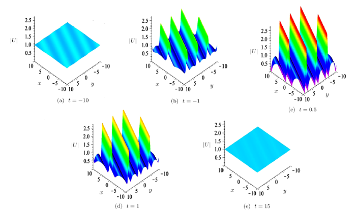
(i) Line breather when $\alpha=0,k=0$. In this case, the first-order breather is a line breather solution, which describes growing and decaying periodic line waves in the $(x,y)$-plane (see Fig.1). When $t\ll0$, waves in this solution grow from a uniform constant background. In the intermediate times, periodic line waves arise from the constant background (see the panels at $t=-10$), and then they attain much higher amplitudes (see the panel at $t=0.5$). At a larger time, these periodic line waves go back to the constant background (see the panel at $t=15$). What is more, the first-order breather solution has qualitatively different behaviors in the same plane with different cycles (see Fig.2).
(ii) Usual breather when $\beta\neq0 \,\mathrm{or}\, \delta\neq0$. When $\beta=0$, the breather is only periodic along the $y$-direction and localized in the $x$-direction (see Fig.2(a)).
When $\delta=0$, the breather is only periodic along the $x$-direction and localized in the $y$-direction (see Fig.2(b)).
When $\beta\neq0,\delta\neq0$, the breather is periodic along a line possessing an acute angle with $x$-axis (see Fig.2(c)). What is more, the first-order breather solutions have qualitatively different behaviors in the $(x,t)$-plane and $(y,t)$-plane with different periods, which are ignored here.
The Second-Order Breather Solution The second-order breather solution can be obtained by taking the parameters in Eq.(5) as follows:
For high-order breather, it has more rich dynamical behaviors. The second-order breather solution is derived analytically, which is shown in Figs.3-5.
 New window|Download| PPT slide
Fig.1The time evolution of the first-order breather $|U|$ Eq.(9) of the Fokas system in the $(x,y)$-plane with parameters given by Eq.(8) and $\zeta_0=0$, $\eta_0=0$, $\alpha=0$, $\beta={1}/{2}$, $k=0$, $\delta=1$.
 New window|Download| PPT slide
Fig.2Three directions of the first-order breather $|U|$ Eq.(9) of the Fokas system in the $(x,y)$-plane at $t=0$ with parameters $\zeta_0=0$, $\eta_0=0$ given by Eq.(8) and (a) $\alpha=1$, $\beta=0$, $k=0$, $\delta={1}/{2}$.(b) $\alpha=0$, $\beta={1}/{2}$, $k=1$, $\delta=0$. (c) $\alpha={1}/{2}$, $\beta={1}/{2}$, $k={1}/{2}$, $\delta=1$.
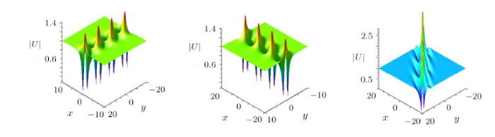
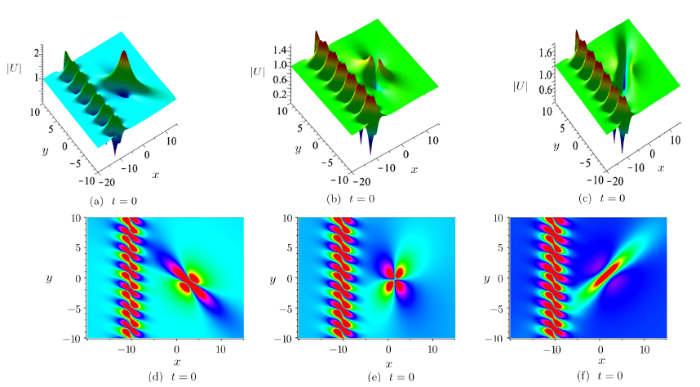
(i) Three different common second-order breather solutions are obtained under different parameters of $P_{i}$, $Q_{i}$, $i=1,2,3,4$. When $P_{i}$ are all pure imaginary numbers and $Q_{i}$ are real constants, that is to say $\alpha_{i}=\delta_{i}=0$ $(i=1,2)$, the second-order breather is only periodic along the $x$-direction and localized in the $y$-direction (see Figs.3(a) and 3(d)).
When $Q_{i}$ are all pure imaginary numbers and $P_{i}$ are real constants, in other words $\beta_{i}=k_{i}=0\;(i=1,2)$, the second-order breather is only periodic along the $y$-direction and localized in the $x$-direction (see Figs.3(b) and 3(e)).
When $\alpha_{1}=\beta_{2}=\delta_{1}=k_{2}=0$, the second-order breather consists of two first-order breather solutions which are propagating along $x$-direction and $y$-direction, respectively (see Figs.3(c) and 3(f)). We can see that they are perpendicular to each other. Furthermore, if $P_{i}$ or $ Q_{i}$ not all pure imaginary numbers or real constants, two first-order breathers in a second-order breather have another qualitatively different behavior, i.e., they propagate along two directions at an acute angle and the direction of propagation is no longer along the $x$ or $y$ axes.
 New window|Download| PPT slide
Fig.3Three types of the second-order breather $|U|$ associated with Eqs.(5) and (11) of the Fokas system in the $(x,y)$-plane at $t=0$ with parameters $\eta_{1}^{0}=\pi$, $\eta_{3}^{0}=-{\pi}/{2}$: (a) $P_{1}=ii/{3}$, $P_{3}=-ii/{3}$, $Q_{1}={1}/{3}$, $Q_{3}={1}/{2}$. (b) $P_{1}={1}/{3}$, $P_{3}={1}/{3}$, $Q_{1}=ii/{3}$, $Q_{3}=ii/{2}$. (c) $P_{1}=ii/{3}$, $P_{3}={1}/{3}$, $Q_{1}={1}/{3} $, $Q_{3}=ii/{2}$.
 New window|Download| PPT slide
Fig.4The time evolution of $|U|$ associated with Eqs.(5) and (11) of the Fokas system in the $(x,y)$-plane with parameters: $\eta_{1}^{0}=\pi$, $\eta_{3}^{0}=-{\pi}/{2}$, $P_{1}=ii/{3}$, $P_{3}={1}/{3}$, $Q_{1}=ii/{3}$, $Q_{3}=ii/{2}$.
(ii) When $\alpha_{1}=\beta_{2}=k_{i}=0$ $(i=1,2)$, in Eq.(11), behaviors similar to that of first-order breather (see Fig.1) can be obtained. In this case, a second-order breather converts to a hybrid of an usual breather and growing-and-decaying periodic line waves. As can be seen in Fig.4, the periodic line waves arise from the constant background and then interact with the moving breather (see $t=-10$ and $t=-3$ panels). Interestingly, on two sides of the breather, the amplitudes of the periodic line waves change at different times. On one side of the breather, the periodic line waves increase rapidly at first (see the panel at $t=-1$). The bigger amplitude means the greater energy.
Then the periodic line waves reach the maximum amplitude for the first time (see the panel at $t=0$), after that, the amplitudes began to decline. At the same time, on the other side of the breather, the amplitudes of the periodic line waves began to increase (see the panel at $t=0.6$) and periodic line waves reach maximum amplitude again at $t=1.2$. Afterwards, the amplitudes began to decline (see the panels at $t=2$ and $t=5$). Finally the periodic line waves disappear in the constant background and only one breather has been remained (see the panel at $t=15$).
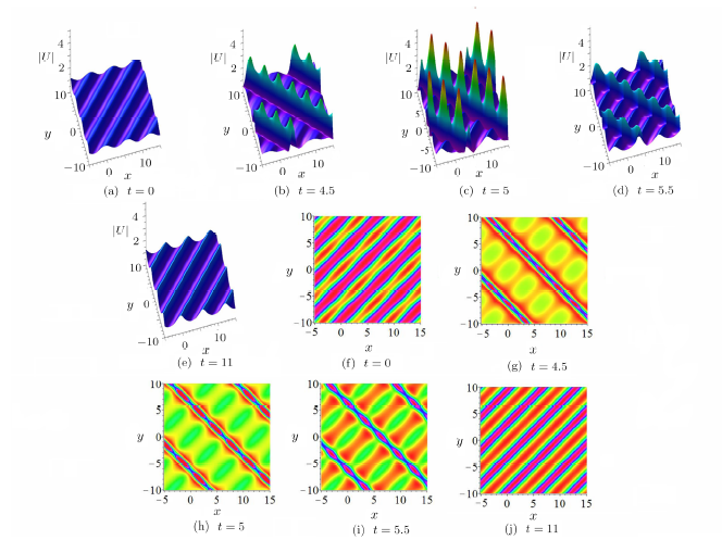
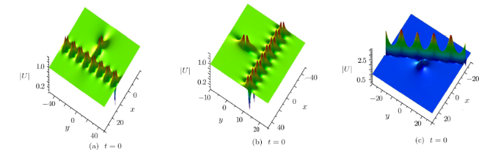
(iii) For $N=4$, more line breather waves will arise and interact with each other, and more complicated wavefronts will form in the interaction region. When $P_{i},Q_{i},(i=1,2,3,4)$ are all pure imaginary numbers, we can construct a hybrid solution consisting of growing-and-decaying periodic line waves and periodic line waves. As we can see in Fig.5, at the intermediate times, periodic line waves arise from the periodic line waves background (see panels at $t=0$ and $t=4.5$) and then interact with the moving periodic line waves. Then, the amplitude reaches its maximum value in a very short period of time and then begins to decline quickly (see panels at $t=5$ and $t=5.5$). It is worth mentioning that, at last, profiles of this solution do not return to the constant plane as shown in Fig.4, i.e., periodic line waves are remained (see panel at $t=11$).
For large even number $N=2n$, by a similar procedure used in above, $n$-th breather can be got, which has more rich dynamical behaviors. We shall discuss it later in a separate paper.
 New window|Download| PPT slide
Fig.5The time evolution of $|U|$ associated with Eqs.(5) and (11) of the Fokas system in the $(x,y)$-plane with parameters: $\eta_{1}^{0}=\pi$, $\eta_{3}^{0}=-{\pi}/{2}$, $P_{1}=ii/{2}$, $P_{3}=i$, $Q_{1}=ii/{2}$, $Q_{3}=-i$.
3 Rational Solutions
Following earlier works in Ref.[46--47], the rational solutions can typically be generated by taking a long wave limits of the obtained $N$-soliton solution given by Eqs.(4) and (5). Indeed, with parameter choices:in Eq.(5), and taking the limit as $P_{j} \rightarrow 0$, then exponential functions $f$ and $g$ are translated into polynomials. Thus rational solutions of the Fokas system can be presented in the following Theorem.
Theorem 1 The Fokas system has $n$-th rational solutions given by
Eqs.(4) adn (5), where functions $f$ and $g$ are given by
the two positive integers $j$ and $k$ are not large than $N$, $\lambda_{j},\lambda_{k}$ are arbitrary real constants, and $\delta_{j}$, $\delta_{k}=\pm1$. Here integer $n= [{N}/{2}]$, $ [{N}/{2}]$ denotes the floor function of $N$.
Remark
(i) When $N=2n$, $\gamma_{j}\gamma_{n+j}=-1$, and $\lambda_j$, $\lambda_{n+j}$ $(j=1,2,\ldots, n)$ are real parameters, the corresponding rational solutions are line rogue waves.
(ii) When $N=2n,\gamma_{j}\gamma_{n+j}=1$, and $\lambda_j$, $\lambda_{n+j}$ $(j=1,2,\ldots, n)$ are complex parameters, the corresponding rational solutions are lumps solution, and a mixture of line rogue wave and lumps elsewhere.
(iii) When $N=2n+1$, the corresponding rational solutions may be singular, thus we do not discuss it more.
When one takes $N=2$ in Theorem~1, then the first-order nonsingular rational solution can be obtained as
It is clear that $U$ and $V$ are smooth when $\lambda_1=\lambda_2$ or $\lambda_1=\lambda_2^*$, which implies two kinds of rational solution:
(i) When $\gamma_1\gamma_2=-1$ and real parameters $\lambda_1$, $\lambda_2$, and $\lambda_{1}=\lambda_{2}$, the rational solution $|U|$ in Eq.(15) is a line rogue wave possessing a varying height. Note that $|U|$ approaches the constant background, whereas at intermediate times, it reaches a much higher amplitude, and finally the line rogue waves disappear the constant background, disappear without a trace that it is different from the moving line solitons, which maintains a perfect profile without any decay during their propagation in the $(x, y)$-plane.
(ii) When $\gamma_1\gamma_2=1$ and complex parameters $\lambda_1$, $\lambda_2$, and $\lambda_1=\lambda_2^{*}$. Let $\lambda_1=a+b i$, $ a$, $b $ are real constants, thus this first-order lump has three different behaviors with different parameters $a$, $b$. Also, if $a=0$, $b\neq0$, in Eq.(15), we can obtain a bi-model lump, $|U|$ has two global maximum points and two global minimum points. If $a$ is a negative number, $b$ is a real number ($a>0$, $b\neq0$) in Eq.(15), we can obtain a dark lump, $|U|$ has two global maximum points and one global minimum point. If $a$ is a positive number, $b$ is a real number ($a<0$, $b\neq0$) in Eq.(15), we can obtain a bright lump, $|U|$ has one global maximum point and two global minimum points.
Note that general higher-order lumps, line rogue waves, and the mixed solution consisting of lumps and rogue waves have been studied in Ref.[31], thus we would not show them again. In next section, we shall focus on the semi-rational solutions, which include several kinds of new hybrid solution.
4 Semi-Rational Solution
Through the above discussion, rational solutions can be generated by taking a long wave limit of all of exponential functions in $f$ and $g$. A natural motivation is to derive the semi-rational solutions by taking a long waves limit of a part of exponential functions in $f$ and $g$ of Eq.(5). Indeed, setting $0<2j<N$ and $1\leq k\leq 2j$,and taking limit $P_{k}\rightarrow 0$ for all $k$, then two functions $f$ and $g$ given by Eq.(5) become a combination of polynomial and exponential functions, which generate semi-rational solutions $U$ and $V$ of the Fokas system through Eqs.(4) and (5).
Furthermore, taking parameter constraints:
when $\lambda_{k}$ are real constants, the corresponding semi-rational solutions are new hybrids of line rogue wave, breather and soliton waves. Also, if $\lambda_{k}$ are complex parameters, the corresponding semi-rational solutions are new hybrids of lump, breather, and soliton waves. Then, the following two types of hybrid solution are considered for the Fokas system.
Type 1 Mixed solution generated from three-soliton solution
In this section, we first consider a type of solution associated with $N=3$. To illustrate semi-rational solutions generated by Eqs.(4) and (5) clearly, taking
and $P_{1}$, $P_{2}\rightarrow 0$,then functions $f$ and $g$ of resulted solutions can be rewritten as
where
and $a_{12}$, $b_{s}$, $\phi_{3}$, $\theta_{s}$, $\eta_{3}$ are given by Eqs.(6) and (14).
This semi-rational solution yields two different mixtures: (i) A mixture of a fundamental lump and first-order dark-soliton when $\gamma_1\gamma_2=1$, $\lambda_1$ and $\lambda_2$ are complex-valued. (ii) A mixture of a fundamental line rogue wave and one-dark-soliton when $\gamma_1\gamma_2=-1$, $\lambda_1$ and $\lambda_2$ are two real parameters.
Case 1 Further,taking parameters in Eq.(19) as
corresponding semi-rational solutions $|U|$ constituting of first-order bright lump and a first-order dark soliton are derived when $a>0,b\neq0$, see Fig.6. As can be seen, the corresponding solution $|U|$ describes the lump in the $(x,y)$-plane, moves and passes the soliton. The first-order lump and first-order dark soliton holds shape during their evolutions although they do opposite movement along a straight line.
Nevertheless, it is observed that the interaction between lump and soliton leads to significant decreasing and increasing of the amplitude around $t=5$ (see Figs.6(b) and 6(d)).
This is an interesting phenomenon in physical systems, which deserves further study in the future.
Furthermore, when $a=0,b\neq0$ and $a<0$, $b\neq0$ two other hybrid solutions can also be obtained, see Fig.7 They are (i) A first-order dark lump and a first-order dark soliton. (ii) A first-order bi-model lump and a first-order dark soliton.
 New window|Download| PPT slide
Fig.6Semi-rational solution $|U|$ associated with Eq.(21) under parameters $\lambda_{1}=1+\i$.
 New window|Download| PPT slide
Fig.7Two kinds of semi-rational solutions $|U|$ associated with Eq.(21). (a) $\lambda_{1}=-1+i$.(b) $\lambda_{1}=i$.
Case 2 Moreover,taking parameters in Eq.(19) as
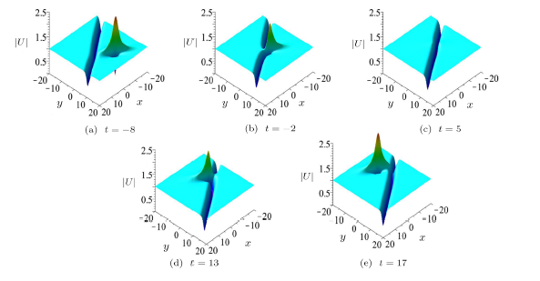
$C$ is an arbitrary real constant. The corresponding semi-rational solution $|U|$ consisted of a fundamental {line} rogue wave and a first-order dark soliton is derived, see Fig.8. As can be seen, the corresponding solution $|U|$ describes the rogue wave in the $(x, y)$-plane, which is growing from and decaying to the soliton background. Six panels in Fig.8 show that the fundamental rogue wave appears from the soliton background (see Figs.8(a) and 8(b)), gradually attains a maximum amplitude at $t = 0 $ of Fig.8(c), and then the amplitude on the other side of the soliton reaches its maximum against $t = 1.5 $ of Fig.8(d), and finally returns back to the soliton plane without a trace (see Figs.8(e) and 8(f)). It is interesting to find that line rogue has two unequal amplitudes in two sides (Figs.8(b) and (8d)).
 New window|Download| PPT slide
Fig.8The semi-rational solution $|U|$ consist of line rogue wave and first-order dark soliton associated with Eqs.(19), (22) and $C=1$.
Type 2 Mixed solution generated from four-soliton solution
To construct semi-rational solution from four-soliton, we have to set parameters in Eq.(5) as the following, namely
and take a limit as $P_{1}$, $P_{2}\rightarrow 0$,then functions $f$ and $g$ of solutions can be rewritten as
where
$$ a_{jk} =\frac{ 2\lambda_{j}P_{k}Q_{k}}{\gamma_{j}\sqrt{2\lambda_{j}P_{k}Q_{k}(P_{k}Q_{k}+2)}+P_{k}\lambda_{j}+Q_{k}} \quad (j=1,2,k=3,4),$$
and $a_{12}$, $b_{s}$, $\theta_{s}$, $\phi_{l}$, $\eta_{l}$, $e^{A_{34}}$ are given by Eqs.(6) and (14). Taking above $f$ and $g$ back into Eq.(4), semi-rational solution is obtained, which has more various dynamical behaviors,such as, mixture of breather and lump, a mixture of rogue wave and breather, one lump on a background of periodic line waves, a line rogue wave on a background of periodic line waves and so on. Below, we only consider four cases of them, namely, a mixture of a lump and one breather, a mixture of line rogue wave, and one breather, line rogue wave and lump on a background of periodic line waves. Next we will illustrate the evolution dynamics of these types of hybrid solutions.
Further, taking parameters in Eq.(24) as
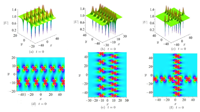
Case 3 When $\gamma_1\gamma_2=1$, $\lambda_2^{*}=\lambda_1$ and parameters in Eq.(25), the solution generated by Eqs.(4) and (24) shows the interaction between a lump and a breather. Let $\lambda_{1}=a+bi$ and discuss the role of $a$ and $b$ to yield different lumps. Similar to the rational solutions which include three kinds of lump, there also exist mixed solutions associated with above lumps. Specifically, three mixed solutions include bright lump when $a>0$, $b\neq0$, bi-model lump when $a=0$, $b\neq0$ and dark lump when $a<0,b\neq0$. So the acquired semi-rational solution $|U|$ is a combination of a bi-model lump lump and breather, a dark lump and breather, a bright lump and breather according to Eqs.(4) and (24) (see Fig.9). Figure~9 confirms the role of $a$ and $b$ to control different pattern of mixed solution, i.e, Fig.9(a) has one bright lump for $a=1$ and $b=1$, Fig.9(b) has one bi-model lump for $a=0$ and $b=1$, Fig.9(c) has one dark lump for $a=-1$ and $b=1$. {Their corresponding density graphs are plotted in Figs.9(d), 9(e), and 9(f), respectively}.
 New window|Download| PPT slide
Fig.9Three kinds of lump combined with breather in the semi-rational solutions $|U|$ associated with Eq.(24) in the $(x,y)$-plane,with parameters $\alpha_{1}=1$, $\beta_{1}={1}/{2}$, $\alpha_{2}=0$, $\beta_{2}=2$, $\eta^{0}_{3}=-4\pi$ in Eq.(25). (a), (d) $a=1$, $b=1$, (b), (e) $a=0$, $b=1$, (c), (f) $a=-1$, $b=1$.
Next, we shall discuss how $\alpha_{i}, \beta_{j},(i=1,2;j=1,2)$ to control the direction of breather in a semi-rational solution associated with Eqs.(24) and (25). There are three typical directions of breather.
(i) The breather is only periodic along the $y$-direction and localized in the $x$-direction (see Fig.10(a)), when $\alpha_{1}\neq0$, $\alpha_{2}=0$, $\beta_{1}=0$, $\beta_{2}\neq0$.
(ii) The breather is only periodic along the $x$-direction and localized in the $y$-direction (see Fig.10(b)), when $\alpha_{1}=0$, $\alpha_{2}\neq0$, $\beta_{1}\neq0$, $\beta_{2}=0$.
(iii) The breather is periodic both along the $x$- and $y$-direction (see Fig.10(c)), when $\alpha_{1}\neq0$, $\alpha_{2}\neq0$, $\beta_{1}\neq0$, $\beta_{2}=0$.
Furthermore, similar profiles of Figs.10(a), 10(b), and 10(c) can be obtained respectively by three choices of parameters: (a) $\alpha_{1}\neq0$, $\alpha_{2}\neq0,\beta_{1}=0,\beta_{2}\neq0$. (b) $\alpha_{1}=0$, $\alpha_{2}\neq0$, $\beta_{1}\neq0$, $\beta_{2}\neq0$. (c) $\alpha_{1}\neq0$, $\alpha_{2}=0$, $\beta_{1}\neq0$, $\beta_{2}\neq0$ or $\alpha_{1}\neq0$, $\alpha_{2}\neq0$, $\beta_{1}\neq0$, $\beta_{2}\neq0$. Significantly, if the $\alpha_{1}$, $\alpha_{2}$ are not zero at the same time, then they must have the same sign, and the positive and negative property of $\alpha_{1}$, $\alpha_{2}$ determines the direction of local propagation of breather solutions on $(x,y)$-plane, $\alpha_{1}$, $\alpha_{2}$ with a positive sign and minus sign, the direction of propagation is just the opposite.
 New window|Download| PPT slide
Fig.10Three directions of the $|U|$ associated with Eq.(24) of the Fokas system in the $(x,y)$-plane with parameters $a=0$, $b=1$. (a) $\alpha_{1}=1$, $\beta_{1}=0$, $\alpha_{2}=0$, $\beta_{2}=1/2$. (b) $\alpha_{1}=0$, $\beta_{1}=1/2$, $\alpha_{2}=1$, $\beta_{2}=0$. (c) $\alpha_{1}=-2$, $\beta_{1}=1$, $\alpha_{2}=-1$, $\beta_{2}=0$.
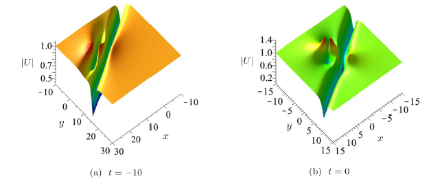
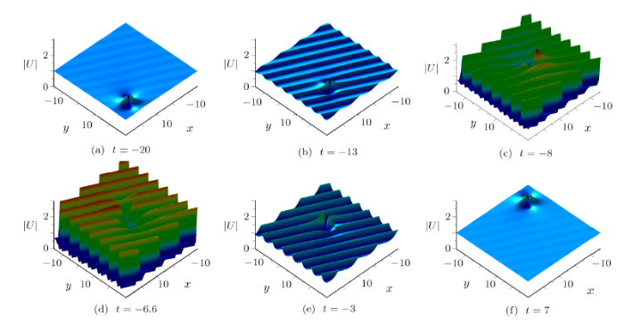
Case 4 When $\gamma_1\gamma_2=1$, set complex parameters $\lambda_2^{*}=\lambda_1$, $\alpha_{1}=0$, $\alpha_{2}=0$, $\beta_{1}\neq0$, $\beta_{2}\neq0$, and select parameters given in Eq.(25),then solution given in Eq.(4) shows the interaction between a lump and growing and decaying periodic line waves. As shown in Fig.11, the lump propagates steadily for a long time. However, the periodic line waves grow and decay within a very short period of time, and the structure of this solution looks very regular. When $t\ll0$, only a lump propagates in the $(x,y)$-plane. In the intermediate times, periodic line waves arises from the background (see panel at $t=-13$), the local maximum amplitude of interaction between lump and periodic lines wave can reach $3.1$ (see panel at $t=-8$), and then they attain much higher amplitudes (see panel at $t=-6.6$). At a larger time, the periodic line waves disappear on the constant background and only the lump has been remained (see panel at $t=7$).
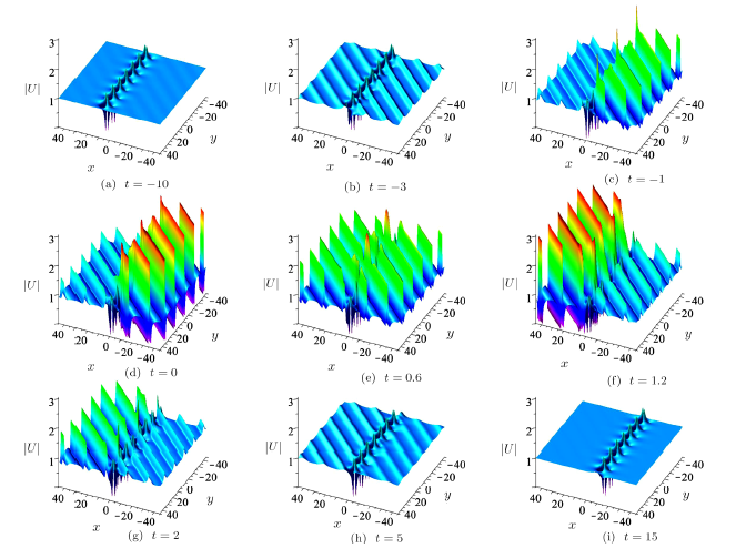
Case 5 When $\gamma_1\gamma_2=-1$, real parameters $\lambda_2=\lambda_1$, and parameters given in Eq.(25), the semi-rational solution given in Eq.(4) can be translated to a hybrid solution consisting of a line rogue wave and a breather. As shown in Fig.12, this kind of hybrid solution describes a line rogue wave interacting with a breather in a short period of time. The line rogue wave arises from the constant background and then interacts with the moving breather (see Figs.12(a) and 12(b)). The amplitudes of the line rogue wave reach maximum in the two sides of the breather at $t=0$ and $t=0.8$ respectively (see Figs.12(c) and (12(d)), which means the structure of the rogue wave is seriously destroyed by the interaction. Then the amplitude begans to drop rapidly, finally the line rogue wave disappears on the constant background and only the breather has been remained (see the panels at $t=5$).
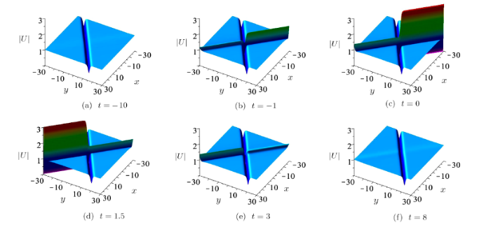
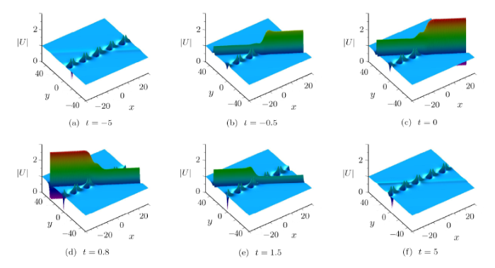
Case 6 When $\gamma_1\gamma_2=-1$, real parameters $\lambda_2=\lambda_1$, and parameters given in Eq.(25), and set $\alpha_{1}=0$, $\beta_{1}\neq0$, $\alpha_{2}=0$, $\beta_{2}\neq0$, then solution in given in Eq.(4) shows the interaction between a line rogue wave and growing and decaying periodic line waves, which is plotted Fig.13. The line rogue wave arises from the periodic background and then interacts with the periodic line waves (see Fig.13(b)). The amplitude of line rogue wave reaches maximum (Fig.13(c)) in a very short time and decreases to background (see Figs.13(d), 13(e), and 13(f)). As can be seen that the maximum amplitude is as high as 7.4 (see Fig.13(c)). The line rogue wave disappears on the periodic line waves background and only the periodic line waves have been remained (see panel at $t=5$).
 New window|Download| PPT slide
Fig.11The time evolution of $|U|$ associated with Eqs.(24) and (25) under the parameters: $\lambda_1=i$, $\eta_{3}^{0}=-\pi$, $\alpha_{1}=0$, $\alpha_{2}=0$, $\beta_{1}=1/2$, $\beta_{2}=1$.
 New window|Download| PPT slide
Fig.12The time evolution of $|U|$ associated with Eqs.(24) adn (25) under the parameters: $\lambda_1=1$, $\eta_{3}^{0}=0$, $\alpha_{1}=0$, $\alpha_{2}=1/2$, $\beta_{1}=1/2$, $\beta_{2}=0$.
5 Summary and Discussion
In this paper, the $n$-th breather of the Fokas system is derived analytically by employing the bilinear method, and the explicit forms of the firstr-order breather solution $U$ are given. With different parameters of $P_{i}$, $Q_{j}$ $(i=1,2,j=1,2)$, the first-order breather is classified as line breather and usual breather, which have been demonstrated in $(x,y)$-planes in Figs.1 and 2. The second-order breather solutions are given graphically in Figs.3--5. By taking a long waves limit of a part of exponential functions in $ f $ and $g$, several interesting hybrid solutions are constructed. The hybrid solutions illustrate various superposed wave structures involving {line} rogue waves, lumps, solitons, and periodic line waves. Under special parameter constraint, corresponding semi-rational solutions $|U|$ are plotted in Figs.6--8. Cases 3-6 of semi-rational generated by four-soliton are plotted in Figs.9--13. As shown in figures, the corresponding solutions of $|U| $ describe the interesting interactions between the lump, line rogue waves, and breathers. It is observed that the interaction between lump and soliton leads to the significant change of the amplitude in the lump. Note that every semi-rational in above just includes two kinds of solutions such as soliton and lump (Figs.6 and 7), or soliton and line rogue waves (Fig.8), or breather and lump (Figs.9 and 10), or line breathers and lump (Fig.11), or breather and line rogue waves (Fig.12), or line breathers and line rogue waves (Fig.13). By the similar way used in this paper, taking larger value of $N$ in $N$-soliton, more complicated patterns will occur in which every semi-rational solution is involved with three or four kinds of solution.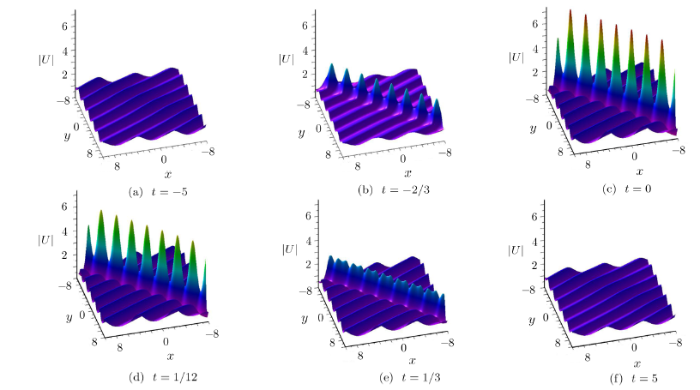 New window|Download| PPT slide
Fig.13The time evolution of semi-rational solution $|U|$ associated with Eqs.(24) and (25) under the parameters: $\lambda_1=1$, $\eta^{0}_{3}=-{\pi}/{2}$, $\alpha_{1}=0$, $\beta_{1}=1$, $\alpha_{2}=0$, $\beta_{2}=-2$.
Reference By original order
By published year
By cited within times
By Impact factor
DOI:10.1016/0167-2789(86)90183-1URL [Cited within: 1]

This book assembles several aspects of soliton theory presently available only in research papers. Attention is focused on the multidimensional problems arising and includes inverse scattering in multidimensions, integrable nonlinear evolution equations in multidimensions and the delta technique. Consideration is given to inverse scattering for the Korteweg-de Vries equation, inverse scattering for integro-differential equations, and the Painleve equations.
[Cited within: 1]
[Cited within: 1]
[Cited within: 1]
[Cited within: 1]
[Cited within: 1]
[Cited within: 1]
[Cited within: 1]
[Cited within: 1]
[Cited within: 1]
[Cited within: 1]
[Cited within: 1]
[Cited within: 2]
[Cited within: 1]
[Cited within: 4]
[Cited within: 1]
[Cited within: 1]
[Cited within: 1]
[Cited within: 1]
[Cited within: 1]
[Cited within: 1]
[Cited within: 1]
[Cited within: 3]
[Cited within: 1]
[Cited within: 1]
[Cited within: 1]
[Cited within: 1]
