 ,2,*, Mohsen Sheikholeslami3
 Corresponding authors: *E-mail:
Received:2018-10-6Online:2019-07-1

Abstract
Keywords:
PDF (3888KB)MetadataMetricsRelated articlesExportEndNote|Ris|BibtexFavorite
Cite this article
Rakesh Kumar, Ravinder Kumar, Reena Koundal, Sabir Ali Shehzad, Mohsen Sheikholeslami. Cubic Auto-Catalysis Reactions in Three-Dimensional Nanofluid Flow Considering Viscous and Joule Dissipations Under Thermal Jump. [J], 2019, 71(7): 779-792 doi:10.1088/0253-6102/71/7/779
Nomenclature
 |
New window|CSV
1 Introduction
In recent years, scientists and engineers who worked in the field of nanoscienceand nanotechnology have revived their interest in exploring the new applicationsof nanomaterials (1 nm--100 nm) and nanostructures. The use of these materialscan provide solutions to numerous environmental and technological challenges suchas solar energy conversion, medicine, catalysis and water purification as pointedout by Anstas and Warner.[1] In this direction, silver colloids have a pointof attraction because of their unique features include good conductivity, chemicalstability, antibacterial nature and catalytic activity.[2] There exists number of method for the preparation and synthesis of silver colloids like chemical, photochemical, and physical but the disadvantages like hazardous waste, expensiveness and toxic substances have unmotivated researchers to use these techniques. Therefore, the focus of researchers in present time is to use green synthesis methods through nontoxic chemicals and environment friendly solvents (water). Sharma et al.[3] in their review report elaborated different green synthesis techniques (Tollens method and polysaccharide method, biological method, irradiation method, and polyoxometalates method) for Ag-NPs. They also incorporated Ag-NPs into other materials (silver-doped hydroxyapatite, polymer-Ag-NPs, poly (vinul alcohol)-Ag-NPs, Ag-NPs on Ti$\text{O}_2$), and illustrated their applications in antibacterial water filter, antimicrobial air filter and treatment of HIV.Silver nanoparticles find their common applications in bone cement, wound dressing, house cleaning chemicals, washing machines, bactericidal coatings in water filters, sprays, respirators and many more (Prabhu and Poulose[4]). Tran et al.[5] described the use of silver nanoparticles in controlling antibacterial, antifungal, antiviral activities, and environmental treatments such as air disinfection, water disinfection (drinking water, groundwater, biological waste water), surface disinfection (plastic catheters antimicrobial surface functionalization, antimicrobial paints, food preservation through antimicrobial packing of paper and silver-impregnated fabrics for clinical clothing). He further demonstrated that in future silver nanoparticles can prove powerful in controlling and preventing microbial infections, waterbrone diseases through magnetic disinfectant system, environmental pollution through effective sorbent and catalyst etc.Carbone et al.[6] explained the role of silver nanoparticles for fresh food packaging in the polymeric matrices. Zhang et al.[7] illustrated various properties of Ag-NPs including anti-angiogenic and anti-cancer agents. Seyhan et al.[8] presented an experimental analysis to examine the influence of functionalized silver nanopaticles over thermal conductivity of water, hexane and ethylene glycol. Peristaltic movement of silver nanofluid through a symmetric channel was analyzed by Abassi et al.[9] Zin et al.[10] reported silver nanofluid flow induced by the oscillation of vertical plate.
On the other hand, nanofluid flows over deformable surfaces with time dependent rotational oscillations have been the concern of several researchers due to the broader spectrum of their applications in food processing, fiber technology, polymer industry, and metallurgical sciences. Matched asymptotic expansion scheme for higher suction was exploited by Wang[11] to understand the flow created by the oscillatory stretching velocities of the sheet. Slip effects in oscillatory environment were investigated by Abbaset al.[12] Impacts of Dufour and Soret on fluctuating flows were analyzed through homotopy analysis method by Zhenget al.[13] Keller box method was employed byJaved et al.[14] to discuss the oblique stagnant flow due to fluctuating plate. Khan et al.[15] accomplished numerical solution for the Bodewadt nanofluid flow caused by a deformable disk.Kumar and Sood[16] explored the uni-directional surface stretching conditions under rotating, oscillatory, and radiating and reacting environment. Impact of rotational oscillations in stretchable nanofluid flow under cubic auto-catalysis reaction environment is illustrated byKumar et al.[17]
In addition to this, work done by velocity against viscous stresses (transformation of mechanicalenergy into thermal energy) is termed as viscous heating of energy. Viscous dissipation mechanism is dominatingin those regions where large velocity gradients exist, for example, in boundary layers or where largevariations in buoyancy force exists or devices which move at high speeds. Also, dissipation term cannot beignored in the flow of highly viscous fluids (polymers, oils), and further,presence of fluctuating velocities on the surface can significantly alter the dissipative heat.Therefore, it becomes important to examine the influence of rotational oscillations onthe dissipative heat through the Eckert number. The pioneering work of Brinkman on viscousdissipation led the researchers to investigate the various aspects of the influence of dissipation.On the other hand, when the energy is transferred from conduction electrons to conductor'satoms via the collision process, heat is always generated. This type of transformation gives riseto an important term called as Joule heating. It plays a healthy role in the design of numerous devices.Singh and Kumar[18] elaborated the combined importance of viscous heating in hydromagneticfluid flow over hot vertical surface.Ram et al.[19] discussed the work of Ref. [18] by adding the aspect of solar radiation.Simultaneous impacts of viscous and Joule heating in nanofluidflow near the stretchable stagnation region are discussed by Nandkeolyar et al.[20]Ahmad and Iqbal[21] inspected the reactions of reactions (heterogeneous/homogeneous) inferrofluid flow with viscous heating. Recently, Khan et al.[22] presented a modified model for heterogeneous and homogeneous reactions in flow of MHD fluid with viscous/Ohmic dissipations.
Though no-slip boundary conditions have been widely used to analyze Navier-Stokes equations yet there are some situations where these conditions fail to predict the exact dynamics of flow field such as thin film flow of light oil relative to the moving plates, thick monolayer of hydrophobic octadecyltrichlorosilane coated on surface, multiple interface problems, non-Newtonian fluid (polymeric materials) flows and flows involving the suspensions of nanoparticles. Rao and Rajagopal[23] represented different models available for the description of slip flows, and they observed that rectilinear and fully developed flow is impossible if velocity has strong dependence on normal stresses. Mehmood and Ali[24] inspected slip condition effects on oscillatory flow in a planer channel.Singh and Kumar[25] investigated fluctuating flow of of reacting and radiating liquidalong vertical porous plate with slip-flow. Kumar and Chand[26] revealed the influencesof Hall currents and velocity slip interface conditions on viscoelastic fluid flow overflat surface. Darcy and rarefaction impacts on radiative-reactive flows insidechannel were examined by Chand et al.[27] For more relevant works, readers can look through (Refs. [28--36]).
The role of Joule and viscous dissipation in the design of various equipments and devices motived us to examine their effects on the nanofluid flow past surfaces for rotational oscillations (time dependent) under slip interface condition environment. To enhance the impact of the analysis, radiation (heat transfer) and cubic autocatalysis chemical reaction effects are also added to the energy and mass diffusion equations respectively.
2 Geometrical Description and Governing Equations
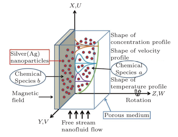
Here we focus ourselves on an unsteady flow of convective nanofluid which is viscous, electrically conducting and incompressible. The nanofluid is formed by the suspension of silver nanoparticles and the flow is subjected to time dependent rotational oscillations of the deforming sheet. In the flow field we consider isothermal cubic homogeneous chemical reaction and on the catalyst surface we consider single isothermal first order heterogeneous chemical reaction (Fig. 1).Fig. 1
 New window|Download| PPT slide
Fig. 1(Color online) Schematic description of the problem.
The homogeneous chemical reaction is defined as:
and heterogeneous reaction on the catalyst surface as
where $a$, $b$ denote the chemical species.
The stretchable sheet in this problem executes oscillations and preserves velocity jumps in normal direction. This effect is mathematically defined as
The sheet temperature is considered to vary periodically along difference of mean temperature of surface and free-stream temperature. the temperature jump is assumed in normal direction. Mathematical form of such temperature is
Following Tiwari and Das[37] and Merkin,[38] the governing radiating and reacting boundary layer equations subjected to velocity/temperature jumps and viscous/Ohmic dissipations under time dependent rotational oscillations can be written as:
Further, the conditions (initial/boundary) have the following mathematical presentation:
For the complete construction of mathematical model elaborating the flow, and heat and mass transfer mechanisms under rotational oscillatory environment, following models are employed (Tiwari and Das model,[37] Hamilton-Crosser model,[39] Makinde and Animasaun,[40] Makinde and Animasaun[41]):
In the dynamics of fluid flows we are interested in those results which are independent from dimensions and thus we introduce the following non-dimensional quantities which will reduce Eqs. (5)--(10) along with Eq. (11) into dimensionless form:
After utilization of these dimensionless quantities, following set of coupled partial differential equations is achieved:
where
$$C_1=(1+0.025\phi+0.015\phi^2)\,, \quad C_2=\phi\Bigl(\dfrac{\rho_s}{\rho_f}\Bigr)-\phi+1\,, C_3=1-\dfrac{3(1-{\sigma_s}/{\sigma_f})\phi} {({\sigma_s}/{\sigma_f}-2)-({\sigma_s}/{\sigma_f}-1)\phi}\,, C_4=\phi\dfrac{(\rho \beta_T)_s}{(\rho \beta_T)_f}-\phi+1\,, \quad C_5=\phi\dfrac{(\rho c_p)_s}{(\rho c_p)_f}-\phi+1\,, \quad C_6=\frac{k_{nf}}{k_f}\,. $$
The dimensionless transformations convert the initial and boundary conditions into
The emerging dimensionless parameters are defined as follows:
$$\;\; M=\frac{\sigma_f B_0^2}{\rho_f c}\,, \quad K=\frac{K^* c}{\nu_f}\,, \quad R=\frac{2\Omega}{c}\,, \;\;Gr=\frac{g(\beta_{T})_{f} (T_w-T_\infty)}{\sqrt{\nu_{f} c^3}}\,, \quad \;\;Pr=\frac{\nu_f}{\alpha_f}\,, \quad Sc=\frac{\nu_f}{D_a}\,, \;\; V_s=L_{1} \sqrt{\frac{c}{\nu_{f}}}\,, \quad Ra=\frac{16\sigma^*T_\infty^3}{3k^*k_f}\,, \quad K_s=\sqrt\frac{\nu_f}{c}\frac{k_r}{D_a}\,, \;\; \delta=\frac{D_b}{D_a}\,, \quad K_c=\frac{k_c C_{\infty}^2}{c}\,, \quad T_s=L_2\sqrt{\frac{c}{\nu_{f}}}\,, \quad Ec=\frac{c\mu_f}{\rho{c_p}}\,. $$
The coefficients which attract engineers most are skin-frictions, Nusselt number and reactant Sherwood numbers. These have the following respective forms in fluid dynamics:
where
$$\quad \tau_{wx}=\mu_{nf}\Bigl(\frac{\partial u}{\partial z}\Bigr)_{z=0}\,, \quad \tau_{wy}=\mu_{nf}\Bigl(\frac{\partial v}{\partial z}\Bigr)_{z=0}\,, \quad q_w=\Bigl(-k_{nf}\frac{\partial T}{\partial z}+q_r\Bigr)_{z=0}\,, \quad j_{wa} = -D_{a}\Bigl(\frac{\partial{C_a}}{\partial{z}}\Bigr)_{z=0}\,, \quad j_{wb} = -D_{b}\Bigl(\frac{\partial{C_b}}{\partial{z}}\Bigr)_{z=0}\,. $$
These coefficients in dimensionless pattern can be readily decided as:
$$\qquad c_{fX}=\Bigl\{\frac{C_1}{(X\cos(\omega t')+V_s({\partial U}/{\partial Z}))^2} \dfrac{\partial U}{\partial Z}\Bigr\}_{Z=0}\,, \qquad c_{fY}=\Bigl\{\frac{C_1}{(X\cos(\omega t')+V_s({\partial U}/{\partial Z}))^2} \frac{\partial V}{\partial Z}\Bigr\}_{Z=0}\,, \qquad Nu_{X}=\Bigl\{\frac{X(-C_6-Ra)}{(\cos(\omega t') +T_s({\partial \theta}/{\partial Z}))}\dfrac{\partial \theta}{\partial Z}\Bigr\}_{Z=0}\,, \qquad Sh_{AX} = \Bigl\{X\dfrac{\partial{A}}{\partial{Z}}\Bigr\}_{Z=0}, \quad Sh_{BX} = \Bigl\{X\dfrac{\partial{B}}{\partial{Z}}\Bigr\}_{Z=0}\,. $$
3 Numerical Scheme
An explicit finite difference approach has been exploited to compute the solutions of involve mathematical expressions. Using explicit finite difference approximation, Eqs. (14)--(19) are written in the following finite difference form:The corresponding boundary conditions are
In the above proposed scheme, $l,m,n$ (subscripts) and $k$ (superscripts) represent the grid nodes in the directions of $X, Y, Z$ and $t'$ respectively. We selected $(X_{\max}, Y_{\max}, Z_{\max}, t'_{\max})=(100, 100, 10, 10)$ after confirming that the conditions may not change outside this range. Here the step-size is considered to be $(\Delta t', \Delta X, \Delta Y, \Delta Z)=(0.005, 10, 10, 0.1)$. The algorithm is presented as follows:
(i) Initially ($t'=0$), we assume that $U_{l,m,n}^k$, $V_{l,m,n}^k$, $W_{l,m,n}^k$,$\theta_{l,m,n}^k$, $A_{l,m,n}^k$, and $B_{l,m,n}^k$ are known.
(ii) we compute, $U_{l,m,n}^{k+1}$, $V_{l,m,n}^{k+1}$, $W_{l,m,n}^{k+1}$,$\theta_{l,m,n}^{k+1}$, $A_{l,m,n}^{k+1}$ and $B_{l,m,n}^{k+1}$ at next time step $(k+1)$ by using above quantities.
(iii) At first, we find $\theta_{l,m,n}^{k+1}$ at every node.
(iv) At second, $U_{l,m,n}^{k+1}$ at every node is computed using $\theta_{l,m,n}^{k+1}$.
(v) Thirdly, $V_{l,m,n}^{k+1}$, $A_{l,m,n}^{k+1}$ and $B_{l,m,n}^{k+1}$ are calculated continuously by employing the updated quantities obtained in all previous steps.
(vi) Lastly, $W_{l,m,n}^{k+1}$ are calculated through the equation of continuity (22).
4 Stability and Convergence
To obtain the stability conditions, we take Fourier expansions for all the quantities ($U, V, \theta, A$, and $B$) at time $t'$ and constant grid sizes as (Von Neumann stability analysis):$$U=\Psi_1(t')e^{\iota\alpha_1 X}e^{\iota\alpha_2 Y}e^{\iota\alpha_3 Z}\,,\\ V=\Psi_2(t')e^{\iota\alpha_1 X} e^{\iota\alpha_2 Y}e^{\iota\alpha_3 Z}\,,\\ \theta=\Psi_3(t')e^{\iota\alpha_1 X}e^{\iota\alpha_2 Y}e^{\iota\alpha_3 Z}\,, \\ A=\Psi_4(t')e^{\iota\alpha_1 X}e^{\iota\alpha_2 Y}e^{\iota\alpha_3 Z}\,, \\ B=\Psi_5(t')e^{\iota\alpha_1 X} e^{\iota\alpha_2 Y}e^{\iota\alpha_3 Z}\,. $$
After single time step, these quantities have the forms:
$$U=\Psi_1'(t')e^{\iota\alpha_1 X}e^{\iota\alpha_2 Y}e^{\iota\alpha_3 Z} \,,\\ V=\Psi_2'(t')e^{\iota\alpha_1 X} e^{\iota\alpha_2 Y}e^{\iota\alpha_3 Z}\,, \\ \theta=\Psi_3'(t')e^{\iota\alpha_1 X}e^{\iota\alpha_2 Y}e^{\iota\alpha_3 Z} \,, \\ A=\Psi_4'(t')e^{\iota\alpha_1 X}e^{\iota\alpha_2 Y}e^{\iota\alpha_3 Z} \,,\\ B=\Psi_5'(t')e^{\iota\alpha_1 X}e^{\iota\alpha_2 Y}e^{\iota\alpha_3 Z}\,.$$
Now, we substitute these assumptions into Eqs. (22)--(27), and obtain the following equations after trivial simplifications:
Further simplification gives rise to a following set of equations:
$$\Psi_3'=A_4\Psi_3+A_5\Psi_1+A_6\Psi_2, \quad \Psi_1'=A_1\Psi_1+A_2\Psi_2+A_3(A_4\Psi_3+A_5\Psi_1+A_6\Psi_2), \\ \Psi_2'=A_1\Psi_2-A_2\Psi_1, \quad \Psi_4'=A_7\Psi_4, \quad \Psi_5'=A_8\Psi_5+A_9\Psi_4,$$
which in matrix form can be written as $ \pmb{AX}=\pmb{B}$. The entries of the coefficient matrix $\pmb{A}$ are:
$$A_1 = 1+U\frac{\bigtriangleup t'}{\bigtriangleup X}(e^{-\iota\alpha_1\bigtriangleup X}-1) +V\frac{\bigtriangleup t'}{\bigtriangleup Y}(e^{-\iota\alpha_2\bigtriangleup Y}-1) +W\frac{\bigtriangleup t'}{\bigtriangleup Z}(1-e^{\iota\alpha_3\bigtriangleup Z}) +\frac{2C_1}{C_2}\frac{\bigtriangleup t'}{\bigtriangleup Z^2}(\cos \alpha_3\bigtriangleup Z-1) \\ \hphantom{A_1 = }-\Bigl( \frac{C_3}{C_2}M+\frac{C_1}{KC_2}\Bigr)\bigtriangleup t', \quad A_2 = R\bigtriangleup t', \quad A_3= Gr\frac{C_4}{C_2}\bigtriangleup t', \\ A_4 = 1+U\frac{\bigtriangleup t'}{\bigtriangleup X}(e^{ - \iota\alpha_1\bigtriangleup X} - 1) +V\frac{\bigtriangleup t'}{\bigtriangleup Y}(e^{ \!-\! \iota\alpha_2\bigtriangleup Y} - 1) +W\frac{\bigtriangleup t'}{\bigtriangleup Z}(1 \!-\! e^{\iota\alpha_3\bigtriangleup Z})+2\frac{1}{Pr} \Bigl(\frac{C_6}{C_5}+\frac{Ra}{C_5}\Bigr)\frac{\bigtriangleup t'}{\bigtriangleup Z^2} (\cos \alpha_3\bigtriangleup Z - 1), \\ A_5 = \Bigl[\frac{C_1}{C_5}(e^{\iota\alpha_3\bigtriangleup Z}-1)^2\frac{\bigtriangleup t'} {(\bigtriangleup z)^2}U+\frac{C_3}{C_5}M\bigtriangleup t' U\Bigr]Ec, \quad A_6 = \Bigl[\frac{C_1}{C_5}(e^{\iota\alpha_3\bigtriangleup Z}-1)^2\frac{\bigtriangleup t'} {(\bigtriangleup z)^2}V+\frac{C_3}{C_5}M\bigtriangleup t' V\Bigr]Ec, \\ A_7 = 1+U\frac{\bigtriangleup t'}{\bigtriangleup X}(e^{-\iota\alpha_1\bigtriangleup X}-1) +V\frac{\bigtriangleup t'}{\bigtriangleup Y}(e^{-\iota\alpha_2\bigtriangleup Y}-1) +W\frac{\bigtriangleup t'}{\bigtriangleup Z}(1-e^{\iota\alpha_3\bigtriangleup Z}) +\frac{2}{Sc}\frac{\bigtriangleup t'}{\bigtriangleup Z^2}(\cos \alpha_3\bigtriangleup Z-1)+K_cB^2, \\ A_8 = 1+U\frac{\bigtriangleup t'}{\bigtriangleup X}(e^{-\iota\alpha_1\bigtriangleup X}-1) +V\frac{\bigtriangleup t'}{\bigtriangleup Y}(e^{-\iota\alpha_2\bigtriangleup Y}-1) +W\frac{\bigtriangleup t'}{\bigtriangleup Z}(1-e^{\iota\alpha_3\bigtriangleup Z}) +\frac{2\delta}{Sc}\frac{\bigtriangleup t'}{\bigtriangleup Z^2}(\cos \alpha_3\bigtriangleup Z-1), \\ A_9 = K_c\bigtriangleup t' B^2. $$
Here $W$ is non-positive and $U$ and $V$ are non-negative everywhere. Eigenvalues of this matrix ($\pmb{A}$) are $\lambda_1={(A_{1}^2+A_{2}^2)}/{A_1}$, $\lambda_2=A_1$, $\lambda_3=A_4$, $\lambda_4=A_7$, and $\lambda_5=A_8$. For stability of present scheme, we should receive $|\lambda_i|\le1$ for $i=1,\ldots,5$. Let $p_1$, $p_2$, and $p_3$ are odd integers, maximum modulus of above mentioned eigenvalues takes place when $\alpha_3\bigtriangleup Z=p_3\pi$, $\alpha_2\bigtriangleup Y=p_2\pi$, and $\alpha_1\bigtriangleup X=p_1\pi$. To satisfy $|\lambda_i|\leq1$, the most negative admissible value is $\lambda_i=-1$. Hence stability conditions are
$$\quad {\chi}+\frac{2C_1}{C_2}\frac{\bigtriangleup t'}{\bigtriangleup Z^2}+ \frac{C_3}{2C_2}M\bigtriangleup t'+\frac{C_1}{2KC_2}-\frac{ R\bigtriangleup t'}{2}\leq 1\,, \quad {\chi}+\frac{2C_1}{C_2}\frac{\bigtriangleup t'}{\bigtriangleup Z^2}+\frac{C_3}{2C_2}M\bigtriangleup t' +\frac{C_1}{2KC_2}\leq 1\,, \quad {\chi}+\frac{2}{Pr}\Bigl(\frac{C_6}{C_5}+\frac{Ra}{C_5}\Bigr)\frac{\bigtriangleup t'} {\bigtriangleup Z^2}\leq 1\,, \quad {\chi}+\frac{2}{Sc}\frac{\bigtriangleup t'}{\bigtriangleup Z^2}+\bigtriangleup t' K_cB^2\leq 1\,, \quad {\chi}+\frac{2\delta}{Sc}\frac{\bigtriangleup t'}{\bigtriangleup Z^2}\leq 1\,. $$
Here ${\chi}=U({\bigtriangleup t'}/{\bigtriangleup X})+V({\bigtriangleup t'}/{\bigtriangleup Y})+|W|({\bigtriangleup t'}/{\bigtriangleup Z})$. Keeping in mind these stability conditions, computations have been carried out to accomplish numerical quantities $(U, V, W, \theta, A, B)$ and $(c_{fX}, c_{fY}, Nu_{X}, Sh_{AX}, Sh_{BX})$ which will be presented and analyzed in next section.
5 Results and Discussion
To acquaint with the mechanisms of heat and mass transportation in the nanofluid flow subjected to viscous and Joule dissipation past deforming surfaces in slip flow regime, numerical quantities obtained in previous section are analyzed through plots and tables for different values of emerging parameters. Thermophysical qualities of silver (Ag) and water (H$_2$O) nanoparticles are presented in Table 1. Accuracy/validation of present outcomes have been portrayed in Table 2. Results of primary and secondary velocity ($U$, $V$), temperature ($\theta$), homogeneous concentration ($A$) and heterogeneous concentration ($B$) are presented graphically. The skin-friction (coefficients) in $X$ and $Y$ directions ($c_{fX}$ and $c_{fY}$), local Nusselt number ($Nu_{X}$) and reactant Sherwood numbers ($Sh_{AX}, Sh_{BX}$) evaluated through tables. Figures and tables are prepared to exhibit the relative importance of two cases to name as NSNF (no-slip nanofluid flow) and SNF (slip nanofluid flow). If not mentioned differently, then values assigned to different parameters are: $\omega=0.1$, $\phi=0.1$, $n = 3$, $Ec = 0.01$, $M = 3$, $K = 3$, $R = 1$, $Ra = 0.4$, $K_s = 1$, $K_c = 0.5$, $V_s = 1$, $T_s = 1$, $Gr = 15$, $Sc = 3.5$, $\delta = 1.2$, and $Pr = 6.07$.Table 1
Table 1Properties of H2O and Ag at 25°C.
| Thermo-physical properties | H2O | Ag |
|---|---|---|
| p(Kg/m3) | 997.1 | 10501 |
| k(W/mK) | 0.613 | 429 |
| cp(J/KgK) | 4179 | 235 |
| (1/K)xl0-5 | 21 | 1.8 |
| Pr | 6.07 | - |
| a(s/m) | 5 x 10~2 | 6.30 x 10⁷ |
New window|CSV
Table 2
Table 2Comparison of the variability of skin friction coefficients (cfx /cfy) and local Nusselt number Nux for different Ra at ω = 0, Vs = 1, Ts = 0, R = 0.5, M = 1, K = 1.5, Ks = 3, Kc = 0.5, Ec = 0.001, ? = 0.1, and Gr = 10.
| Kumar and Sood[16] | Present study | |
|---|---|---|
| Ra | (cfx, cfy, Nux) | (cfx, cfy, Nux) |
| 0.8 | (0.723 606, -0.716 842, 0.755 381) | (0.7463406, -0.7629039, 0.723 199 5) |
| 1.5 | (0.766 609, -0.744 827, 0.944 736) | (0.7834152, -0.7919051, 0.8998278) |
| 2 | (0.791274, -0.761 166, 1.063168) | (0.804 576 8, -0.808 7661, 1.009 455) |
| 3.5 | (0.846 564, -0.798 565, 1.363 603) | (0.851706 5, -0.847143 2, 1.284 967) |
New window|CSV
5.1 Effect of Oscillation Frequencies ($\omega$)
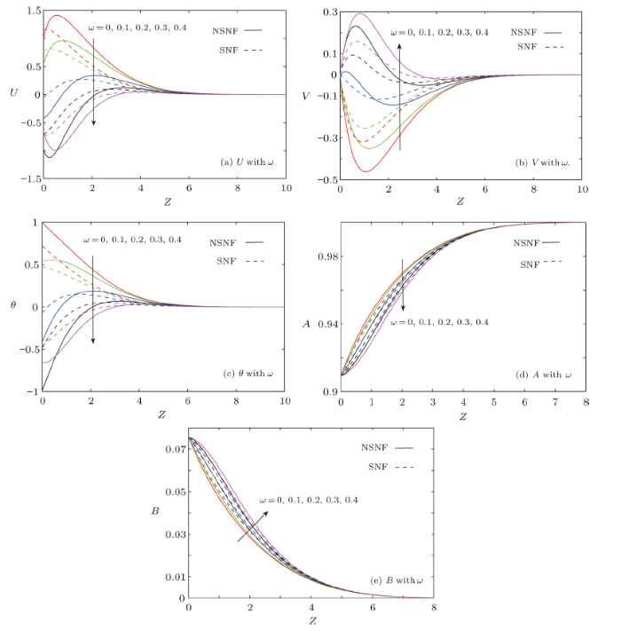
Figures 2(a)--2(e) illustrate the influence of $\omega$ on the profiles of ($U$, $V$), $\theta$ and $A$ and $B$. Under both the cases, $U$ and $\theta$ are reduced with $\omega$ but $V$ is enhanced with it. As magnitude of frequency of oscillation is raised, primary velocity starts to behave as secondary velocity and reverse flow patterns start to appear in $U$ component. Thus to curtail reverse flow, optimal value of $\omega$ can be exploited. Further, with the increasing $\omega$, negative temperature profiles appear owing to inverted Boltzmann distribution. Same negative profiles have been obtained by Kumar and Sood.[16] In the vicinity of the sheet velocity is higher in SNF situation in comparison to NSNF case. Therefore in SNF case, more heat will be transferred by this augmented velocity component and the result will be reduced temperature. That is why, temperature profiles are lowered in SNF case. Homogeneous concentration ($A$) is reduced whereas a growth is noticed in heterogeneous concentration $B$ with increasing oscillation frequency.Fig. 2
 New window|Download| PPT slide
Fig. 2(Color online) Outcomes of frequency of oscillation ($\omega$).
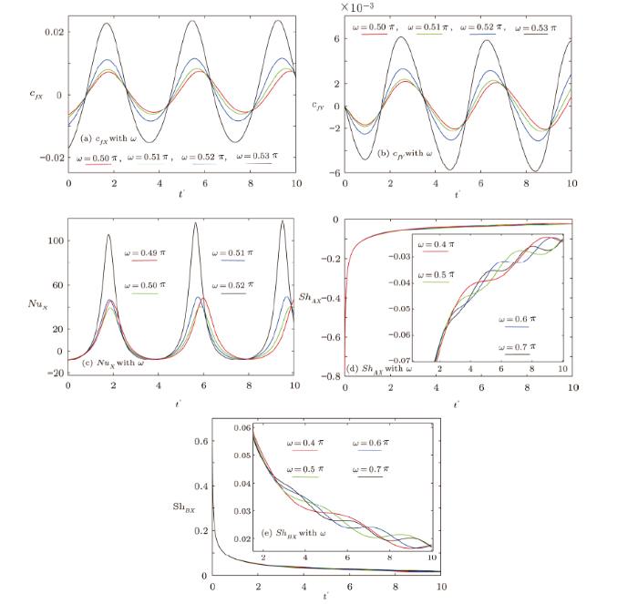
Figures 3(a)--3(e) portray the control of frequency of oscillation on $c_{fX}$, $c_{fY}$, $Nu_X$, $Sh_{AX}$, and $Sh_{BX}$. As expected, fluctuating nature of $c_{fX}$, $c_{fY}$, and $Nu_X$ is encountered when time constraint is varied. Whereas prominent oscillations in $Sh_{AX}$ and $Sh_{BX}$ are disclosed for $t'>2$. Interesting part prevails at $\omega=(52/100)\pi$ where $|c_{fX}|$ is not altered by time, but minima of $c_{fY}$ is augmented for higher values of $t'$. Peak points of $Nu_X$ exist at $\omega=(53/100)\pi$, which get uplifted with $t'$ by maintaining constant minima.
Fig. 3
 New window|Download| PPT slide
Fig. 3(Color online) Outcomes of frequency of oscillation ($\omega$) against $t'$.
5.2 Effect of Eckert Number ($Ec$)
Figures 4(a)--4(c) determine the effect of Eckert number on ($U$, $V$) and $\theta$ in the boundary layer. Magnitudes of primary and secondary velocities as well as temperature are elevated with the heightened values of $Ec$ in both the cases. Since, Eckert number is the ratio of the product of stretching rate and kinematic viscosity to temperature difference, therefore as $Ec$ is boosted up, physically fluid velocity should increase. On the other hand, higher values of $Ec$ increase viscous dissipation impact therefore fluid temperature is augmented.Fig. 4
 New window|Download| PPT slide
Fig. 4(Color online) Outcomes of Eckert number ($Ec$).
5.3 Effect of Volume Fraction of Nanoparticles ($\phi$)
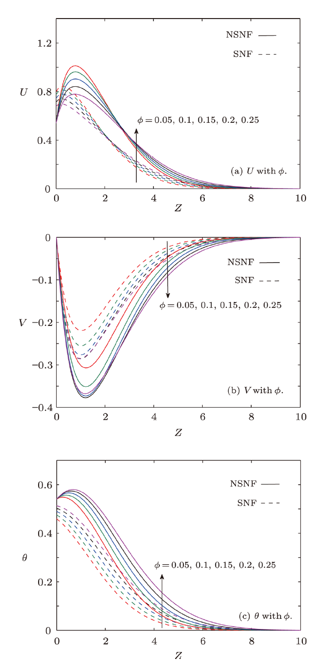
Figures 5(a)--5(c) elucidate variations in the profiles of $U$, $V$, and $\theta$ with respect to $\phi$ in SNF and NSNF cases. It is noted that magnitude of $V$ and $\theta$ are strengthened with $\phi$ everywhere inside the boundary layer, however $U$ is diminished in the vicinity of sheet. The behavior of $U$ is altered after crossing the point of inflections in the flow field. Physically this is true because increasing values of $\phi$ raise nanofluid viscosity which hampers the resultant velocity, that is why, $U$ is compressed.Fig. 5
 New window|Download| PPT slide
Fig. 5(Color online) Outcomes of nanoparticles volume fraction ($\phi$).
5.4 Effect of Homogeneous/Heterogeneous Reaction Parameters ($K_c/K_s$)
Figures 6(a)--6(d) highlight the importance of $K_c$ and $K_s$ on the concentrations profiles $A$ and $B$. It is examined that homogeneous concentration enhances and heterogeneous concentration retards with the increasing generative homogeneous reactions $(K_c<0)$. However, opposite trends are noticed with respect to destructive homogeneous reactions $(K_c>0)$. It is also deduced from mentioned figures that constructive and destructive heterogeneous reactions $(K_s<0, K_s>0)$ have similar effects on $A$ and $B$ as $K_c<0$ and $K_c>0$ have on $A$ and $B$.Fig. 6
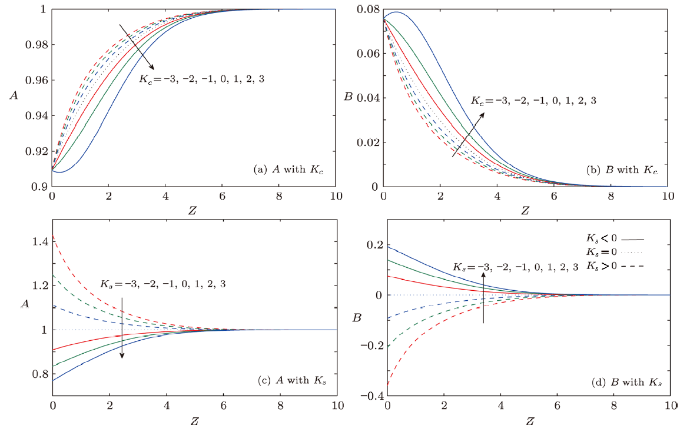 New window|Download| PPT slide
Fig. 6(Color online) Outcomes of $K_c$ and $K_s$ on concentrations ($A$ and $B$).
5.5 Effect of Schmidt Number ($Sc$)
Figures 7(a)--7(d) accentuate the relevance of Schmidt number $Sc$ in the distribution of homogeneous and heterogeneous concentrations profiles. Schmidt number tends to raise the homogeneous concentration profiles $(A)$ in both the cases of generative and destructive homogeneous reaction parameters, on the other hand, it tends to lower the heterogeneous concentration profiles $(B)$. An interesting effect of $Sc$ has been noticed in the case of heterogeneous reactions. Homogeneous concentration profiles $(A)$ are diminished with respect to $K_s<0$ and elevated with $K_s>0$. However, opposite behavior has been detected in the case of heterogeneous concentration profiles $(B)$.Fig. 7
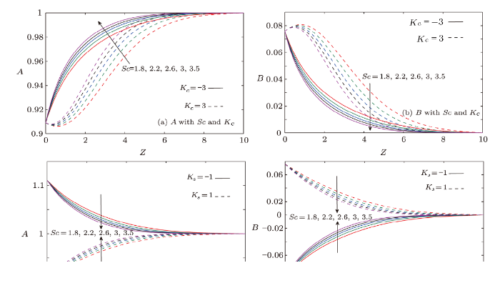 New window|Download| PPT slide
Fig. 7(Color online) Outcomes of Schmidt number ($Sc$) on concentrations on $A$ and $B$ for different $K_s$ and $K_c$.
5.6 Effect on Skin-Friction, Reactant Sherwood Numbers and Nusselt Number
Effects of $M$, $K$, and $R$ on skin friction factors $(c_{fX}, c_{fY})$, reactant Sherwood numbers $(Sh_{AX}, Sh_{BX})$ and Nusselt number $(Nu_{X})$ are presented in Table 3 and Table 4 to emphasize the relative importance of slip nanofluid flow (SNF) over no slip nanofluid flow (NSNF). In SNF case, magnitudes of $c_{fX}$ and $c_{fY}$ are reduced with $M$ and $K$, whereas, $R$ reduces $c_{fX}$ and enhances $c_{fY}$ in magnitudes. $Nu_{X}$ is aggrandized by $K$, but $M$ and $R$ curtail it. Magnitudes of $Sh_{AX}$ and $Sh_{BX}$ are lowered with $M$, $K$, and $R$. In general, increasing $M$ and $K$ have the tendency to raise skin friction coefficients, but here time dependent rotational oscillations have played a predominant role in inverting this physical phenomenon. It is pertinent to mention here that in NSNF case, the quality of trends are same as that of SNF case but the major difference is that the magnitudes of skin-friction coefficients are much smaller and rates of heat transfer are much higher in SNF situation in comparison to NSNF case.Table 3
Table 3Variability of skin friction coefficients (cfx/cfy), local Nusselt number Nux and Sherwood numbers (SHax/SHbx) for different values of M, K and R in SNF case (Vs = Ts≠ 0).
| M | K | R | (cfx,Cfy) | (Nux) | (ShAx, ShBx) |
|---|---|---|---|---|---|
| 3 | 3 | 1 | (0.007 3612, -0.020 193 3) | 2.433 326 | (-0.038 619 2, 0.028 477 6) |
| 5 | (0.0030690, -0.0132055) | 2.225 189 | (-0.036 692 1, 0.027 064 8) | ||
| 7 | (-0.000 118 5, -0.009 4916) | 2.161 725 | (-0.034 889 0, 0.025 714 5) | ||
| 9 | (-0.0025423,-0.0072348) | 2.157 807 | (-0.033 4315, 0.024 618 1) | ||
| 3 | 3 | 1 | (0.007 361 2, -0.020 193 3) | 2.433 326 | (-0.038 619 2, 0.028 477 6) |
| 5 | (0.003 253 7, -0.017 108 7) | 2.881 315 | (-0.035 566 2, 0.026 165 5) | ||
| 7 | (0.000 375 8, -0.014 868 1) | 3.087 055 | (-0.0336178, 0.0246968) | ||
| 9 | (-0.001 788 5, -0.013 173 4) | 3.186 164 | (-0.032 244 4, 0.023 664 7) | ||
| 3 | 3 | 0.8 | (0.007 426 0, -0.016 240 6) | 2.613 552 | (-0.039 723 3, 0.029 341 0) |
| 1.5 | (0.006 951 2, -0.029 473 9) | 2.000 986 | (-0.035 695 7, 0.026198 1) | ||
| 2.2 | (0.005 863 3, -0.040 377 6) | 1.507 200 | (-0.031 621 7, 0.023 041 5) | ||
| 2.9 | (0.004 374 1, -0.048 420 4) | 1.189 210 | (-0.028 070 7, 0.020 314 6) |
New window|CSV
Table 4
Table 4Variability of skin friction coefficients (cfx/cfy), local Nusselt number (Nux) and Sherwood numbers (SHAx/SHBx) for different values of M,K and R in NSNF case (VS = Ts = 0)..
| M | K | R | (cfx, cfy) | Nux | (ShAx, ShBx) |
|---|---|---|---|---|---|
| 3 | 3 | 1 | (0.045 101 1, -0.024 203 7) | -2.375 846 | (-0.041 399 7, 0.030 716 5) |
| 5 | (0.026 255 1, -0.015 443 8) | -2.623 367 | ( -0.040 109 6, 0.029 747 7) | ||
| 7 | (0.011 882 7, -0.011 147 8) | -2.795 299 | (-0.038 481 6, 0.028 496 4) | ||
| 9 | (0.000 452 8, -0.008 642 0) | -2.890 901 | (-0.037 020 4, 0.027 372 0) | ||
| 3 | 3 | 1 | (0.045 101 1, -0.024 203 7) | -2.375 846 | (-0.041 399 7, 0.030 716 5) |
| 5 | (0.028 237 1, -0.020 725 5) | -1.356 246 | (-0.038 538 8, 0.028 486 3) | ||
| 7 | (0.015 826 4, -0.018 241 1) | -0.886 092 7 | (-0.036 616 4, 0.026 999 8) | ||
| 9 | (0.005 970 6, -0.016 373 1) | -0.6541395 | (-0.035 200 7, 0.025 911 5) | ||
| 3 | 3 | 0.8 | (0.045 654 8,-0.019 4512) | -1.876 567 | (-0.042 796 2, 0.031 816 8) |
| 1.5 | (0.042 513 4, -0.035 346 5) | -3.640 277 | (-0.037 654 8, 0.027 769 9) | ||
| 2.2 | (0.036 490 6, -0.048 277 0) | -5.198112 | (-0.032 306 3, 0.023 578 2) | ||
| 2.9 | (0.028 799 6, -0.057 539 9) | -6.247421 | ( -0.027 549 8, 0.019 877 5) |
New window|CSV
Influences of $Ra$, $\omega$, and $Ec$ on $(c_{fX}, c_{fY})$, $(Nu_{X})$, and $(Sh_{AX}, Sh_{BX})$ are highlighted in Table 5 and Table 6. In SNF case, magnitudes of $(c_{fX}, c_{fY})$ and $(Sh_{A}, Sh_{B})$ are hiked up by $Ra$ and $Ec$, however $Nu_{X}$ is depressed with $Ra$ and $Ec$. Magnitudes of reactant Sherwood numbers $(Sh_{AX}, Sh_{BX})$ are also hampered with $\omega$. The most interesting phenomenon is created by the rotational oscillations of the stretching surface. For lower values of frequency of oscillations, skin-friction coefficients are raised but for broader values of $\omega$ these coefficients ($c_{fX}, c_{fY}$) are reduced. Same trends can be seen in Table 6 for NSNF case. It is worthy to indicate that frequency of oscillation $(\omega=0.2)$ can be exploited to turn the behaviour of skin friction coefficients and Nusselt number. Maxima of rate of heat transfer $(Nu_{X})$ exists at $\omega=0.2$. Here, the point of interest is that magnitudes of $c_{fX}, c_{fY}$ and $Sh_{AX}, Sh_{BX}$ are smaller, and $Nu_{X}$ are larger in SNF case than in NSNF case.
Table 5
Table 5Variability of skin friction coefficients (cfX/cfY ), local Nusselt number (NuX) and Sherwood umbers (ShAX/ShBX) for different values of Ra, ω and Ec in SNF case (Vs = Ts ≠ 0).
| Ra | Ec | (cfx,cfy) | Nux | (ShAx,SHbx) | |
|---|---|---|---|---|---|
| 0.4 | 0.1 | 0.01 | (0.007 3612, -0.020 193 3) | 2.433 326 | (-0.038 619 2, 0.028 477 6) |
| 0.8 | (0.008 089 9, -0.021 037 7) | 2.376 643 | (-0.039 506 8, 0.029 172 2) | ||
| 1.2 | (0.008 640 9, -0.021 689 4) | 2.287593 | (-0.040 210 4, 0.029 724 8) | ||
| 1.6 | (0.009 073 2, -0.022 209 5) | 2.177 142 | (-0.040 784 4, 0.030 177 0) | ||
| 0.4 | 0 | 0.01 | (0.001 426 6, -0.008 416 9) | 6.586 285 | (-0.042 664 5, 0.031 493 4) |
| 0.1 | (0.007 3612,-0.020 193 3) | 2.433 326 | (-0.038 619 2, 0.028 477 6) | ||
| 0.2 | (0.024 535 3, -0.007 576 3) | 77.074 29 | (-0.028 666 2, 0.021 074 7) | ||
| 0.3 | (0.002 929 3, 0.004 086 5) | 17.846 68 | (-0.018 548 0, 0.013 573 3) | ||
| 0.4 | (-0.001 454 9, 0.011 679 3) | 7.654724 | (-0.014 276 9, 0.010 407 0) | ||
| 0.4 | 0.1 | 0.005 | (0.005 915 3, -0.018 928 4) | 3.714268 | (-0.037 574 7, 0.027 679 0) |
| 0.01 | (0.007 3612,-0.020 193 3) | 2.433 326 | (-0.038 619 2, 0.028 477 6) | ||
| 0.015 | (0.009 189 5, -0.021 769 2) | 0.957539 | (-0.039 940 3, 0.029 488 9) | ||
| 0.02 | (0.011 579 5, -0.023 784 6) | -0.768 031 | (-0.041 674 2, 0.030 818 1) |
New window|CSV
Table 6
Table 6Variability of skin friction coefficients (cfX/cfY ), local Nusselt number (NuX) and Sherwood numbers (ShAX/ShBX) for different values of Ra, ω and Ec in NSNF case (Vs = Ts = 0).
| Ra | Ec | (cfx, cfy) | Nux | (SHax , SHbx) | |
|---|---|---|---|---|---|
| 0.4 | 0.1 | 0.01 | (0.045 101 1, -0.024 203 7) | -2.375 846 | (-0.041399 7, 0.030 716 5) |
| 0.8 | (0.045 619 7,-0.024 587 7) | -2.846 729 | (-0.0418108, 0.031060 6) | ||
| 1.2 | (0.045 9612,-0.024 864 3) | -3.283 800 | (-0.042 1175, 0.031 318 8) | ||
| 1.6 | (0.046 196 2,-0.025 0721) | -3.692 801 | (-0.042 355 6, 0.031520 2) | ||
| 0.4 | 0 | 0.01 | (0.0172209,-0.0106230) | 5.256952 | (-0.047741 3, 0.035 475 5) |
| 0.1 | (0.045 101 1, -0.024 203 7) | -2.375 846 | (-0.041399 7, 0.030 716 5) | ||
| 0.2 | (0.012 8541, 0.006 220 2) | 29.824 84 | (-0.025 944 3, 0.019 155 2) | ||
| 0.3 | (-0.0099312, 0.007 8093) | 13.42764 | (-0.0112600, 0.008 216 7) | ||
| 0.4 | (-0.033 7732,0.0176608) | -0.634210 | (-0.0078021, 0.005 619 4) | ||
| 0.4 | 0.1 | 0.005 | (0.040 895 9,-0.022 833 3) | 0.3041929 | (-0.040 5021, 0.029 998 5) |
| 0.01 | (0.045 101 1, -0.024 203 7) | -2.375 846 | (-0.041399 7, 0.030 716 5) | ||
| 0.015 | (0.050 912 6,-0.026 083 2) | -6.063 425 | (-0.042 5664, 0.031652 3) | ||
| 0.02 | (0.059 643 9,-0.028 856 7) | -11.625 26 | (-0.044 174 9, 0.032 946 1) |
New window|CSV
6 Conclusions
Three-dimensional boundary layer equations for the nanofluid flow under time dependent rotational oscillations are proposed considering viscous/ohmic dissipations, and slip conditions on the interface (wall-fluid). For novelty, cubic auto-catalysis chemical reactions in mass diffusion equations and radiative heat transfer in energy equation are incorporated. The assumptions and algorithm for the solution of governing equations are presented. Based on above results captured from this study, following conclusions are made:$\bullet$ Increasing values of $\omega$ tend to reverse the flow behaviour as well as distribution of temperature inside the boundary layer.
$\bullet$ Eckert number $Ec$ augments nano-fluid velocity as well as its temperature.
$\bullet$ Nano-fluid temperature is lesser in SNF case in contrast to NSNF case, whereas ($U$, $V$) are larger in SNF problem as compared NSNF situation.
$\bullet$ Higher $c_{fX}$ and $c_{fY}$ due to $M$ and $K$ can be curtailed by introducing time dependent rotational oscillations on the surface.
$\bullet$ Interface slip conditions help in reducing skin-friction (coefficients), and in enhancing multiple transfer rates.
$\bullet$ Critical frequency $\omega=(52/100)\pi$ or $\omega=(53/100)\pi$ is useful for enhanced transfer rates (heat/mass).
Thus we can say that interface velocity slip and temperature jump in presence of viscous/Ohmic dissipations play a substantial role in controlling skin-friction (coefficients) and heat/mass transportation rates when treated as a function of time.
Reference By original order
By published year
By cited within times
By Impact factor
[Cited within: 1]
[Cited within: 1]
[Cited within: 1]
[Cited within: 1]
[Cited within: 1]
[Cited within: 1]
[Cited within: 1]
[Cited within: 1]
[Cited within: 1]
[Cited within: 1]
[Cited within: 1]
[Cited within: 1]
[Cited within: 1]
[Cited within: 1]
[Cited within: 1]
[Cited within: 3]
[Cited within: 1]
[Cited within: 2]
[Cited within: 1]
[Cited within: 1]
[Cited within: 1]
[Cited within: 1]
[Cited within: 1]
[Cited within: 1]
[Cited within: 1]
[Cited within: 1]
[Cited within: 1]
[Cited within: 1]
[Cited within: 1]
[Cited within: 2]
[Cited within: 1]
[Cited within: 1]
[Cited within: 1]
[Cited within: 1]
