HTML
--> --> -->Large ensembles (LEs) of climate simulations offer a powerful approach to assess climate change detection. While single-model LEs target the uncertainty arising from internal climate variability (i.e., from natural interactions in the coupled ocean–atmosphere–land–biosphere–cryosphere system), multi-model ensembles also include structural uncertainty (arising from differences in model formulation), but offer, in turn, unique insights on the forced climate response since they provide information from the perspective of diversified efforts to simulate the climate system. Despite the exclusive value of a single-model LE in addressing more specifically the intrinsic climate variability, there is no evidence that any particular model is more realistic at climate projections than others of its class (Deser et al., 2020).
In LE analysis, the ensemble mean, which is referred to as the signal (S), represents the forced response (i.e., the anthropogenic climate change); while the ensemble spread, or noise (N), represents the uncertainty arising from two sources: internal variability and model structural differences. Therefore, ensemble spread in single-model LE arises only from internal variability, while in multi-model LEs the spread is due to both the model configuration and internal variability. A third source of projection uncertainty is associated with the possible radiative forcing scenarios.
Little et al. (2015) assessed the sources of uncertainty for modeled sea level change in CMIP5 projections and suggested that the combined effect of temperature biases, upper-ocean stratification, and vertical mixing impact the thermosteric sea change across models. Moreover, they discuss that differences in atmospheric models lead to discrepancies in surface fluxes and feedback, which increase uncertainties in multi-model LEs.
The Intergovernmental Panel on Climate Change (IPCC) assessments rely on multi-model climate projections based on new alternative development scenarios of future emissions and land-use changes [the Shared Socioeconomic Pathways, or SSPs (O’Neill et al., 2016) and the forcing levels of CMIP5’s Representative Concentration Pathways, or RCPs (van Vuuren et al., 2011)], produced with integrated assessment models participating in phase 6 of the Coupled Model Intercomparison Project (CMIP6; Eyring et al., 2016).
The SSPs’ narrative① illustrate possible anthropogenic drivers of climate change over the 21st century (departing from the historical runs) ranging from sustainable to fossil-fueled development (Riahi et al., 2017):
● SSP1 — Sustainability — Taking the Green Road: Low challenges to mitigation and adaptation;
● SSP2 — Middle of the Road: Medium challenges to mitigation and adaptation;
● SSP3 — Regional Rivalry — A Rocky Road: High challenges to mitigation and adaptation;
● SSP4 — Inequality — A Road Divided: Low challenges to mitigation, high challenges to adaptation;
● SSP5 — Fossil-fueled Development — Taking the Highway: High challenges to mitigation, low challenges to adaptation.
Beyond improving the understanding of the climate system and characterizing societal risks and response options, numerical climate change projections provide relevant information regarding the emergence of anthropogenically forced trends above internal variability (Carson et al., 2019). This particular time, when S exceeds N above a particular threshold with no turning back below it, is referred to as the time of emergence (ToE).
The dynamic sea level (DSL) is the spatiotemporally dependent sea surface topography referenced to the Earth’s geoid and it is influenced by ocean currents, local mass balance and density changes in the water column (Cazenave and Remy, 2011; Griffies and Greatbatch, 2012; Gregory et al., 2013; Richter et al., 2013). DSL does not count for global mean SLR and does not contain any other sea level signal, such as zero global mean thermosteric sea level, land ice melt, land motion, or inverse barometer effects; it is defined to have a global mean of zero (Gregory et al., 2019). According to several past studies, regional sea level changes are usually detected by examining DSL changes (e.g., Slangen et al., 2014; Bordbar et al., 2015; Hu and Bates, 2018).
Here, we investigate the most up-to-date projected DSL for the 21st century as simulated by state-of-the-art global climate models and Earth System Models (ESMs) under the auspices of the CMIP6 project (Table 1). First, the results from the 50-member CanESM5 ensemble (Swart et al., 2019) are assessed for two historical CMIP6 experiments: historical (1850 to 2014, full-forcing) and historical-natural (1850 to 2020; natural-only with no anthropogenic forcing). The trends in sterodynamic sea-level [DSL plus global mean thermosteric sea-level, as defined in Gregory et al. (2019)] from these experiments are compared for consistency against satellite altimetry data from the Archiving, Validation and Interpretation of Satellite Oceanographic data (AVISO+,
| Model # | Model name | Model center | Model reference |
| 1 | ACCESS-CM2 | CSIRO-ARCCSS | (Kiss et al., 2020) |
| 2 | ACCESS-ESM1-5 | CSIRO | (Ziehn et al., 2020) |
| 3 | BCC-CSM2-MR | BCC | (Wu et al., 2019) |
| 4 | CAMS-CSM1-0 | CAMS | (Rong et al., 2018) |
| 5 | CanESM5-CanOE | CCCma | (Swart et al., 2019) |
| 6 | CanESM5* | CCCma | (Swart et al., 2019) |
| 7 | CESM2 | NCAR | (Lauritzen et al., 2018) |
| 8 | CESM2-WACCM | NCAR | (Liu et al., 2018) |
| 9 | CNRM-CM6-1 | CNRM-CERFACS | (Voldoire et al., 2019) |
| 10 | CNRM-CM6-1-HR | CNRM-CERFACS | (Voldoire et al., 2019) |
| 11 | CNRM-ESM2-1 | CNRM-CERFACS | (Séférian et al., 2019) |
| 12 | EC-Earth3 | EC-Earth-Consortium | (Wyser et al., 2019) |
| 13 | EC-Earth3-Veg | EC-Earth-Consortium | (Wyser et al., 2019) |
| 14 | FGOALS-g3 | CAS | (Li et al., 2020) |
| 15 | GISS-E2-1-G | NASA-GISS | (Kelley et al., 2020) |
| 16 | HadGEM3-GC31-LL | MOHC | (Roberts et al., 2019) |
| 17 | INM-CM4-8 | INM | (Volodin et al., 2019a) |
| 18 | INM-CM5-0 | INM | (Volodin et al., 2019b) |
| 19 | IPSL-CM6A-LR | IPSL | (Lurton et al., 2020) |
| 20 | MIROC-ES2L | MIROC | (Hajima et al., 2019) |
| 21 | MIROC6 | MIROC | (Tatebe et al., 2019) |
| 22 | MPI-ESM1-2-LR | MPI-M | (Mauritsen et al., 2019) |
| 23 | MPI-ESM1-2-HR | MPI-M DWD DKRZ | (Müller et al., 2018) |
| 24 | MRI-ESM2-0 | MRI | (Yukimoto et al., 2019) |
| 25 | NorESM2-LM | NCC | (Seland et al., 2020) |
| 26 | NorESM2-MM | NCC | (Seland et al., 2020) |
| 27 | UKESM1-0-LL | MOHC | (Sellar et al., 2019) |
| * Results used in both datasets, the CanESM5 and the CMIP6 multi-model ensembles. | |||
Table1. Earth System Models used.
Projected DSL responses to three distinct SSPs are then presented for the 50-member CanESM5 ensemble mean and a CMIP6-27-model ensemble mean. The three CMIP6 scenarios used are: the SSP1-2.6 (sustainability, low emissions, mitigation – year 2100 forcing of 2.6 W m?2), SSP3-7.0 (business as usual, medium to high emissions — year 2100 forcing of 7.0 W m?2), and SSP 5-8.5 (fossil-fueled development, high emissions — year 2100 forcing of 8.5 W m?2). Our goal is to provide a global picture of projected regional DSL based on the agreement between both the CanESM5 and the CMIP6-27-model ensemble sets. Furthermore, we discuss the projected DSL outcomes from distinct SSP scenarios and how they differ between the single- and multi-model ensemble approaches.
2
2.1. Initial condition CanESM5 ensemble
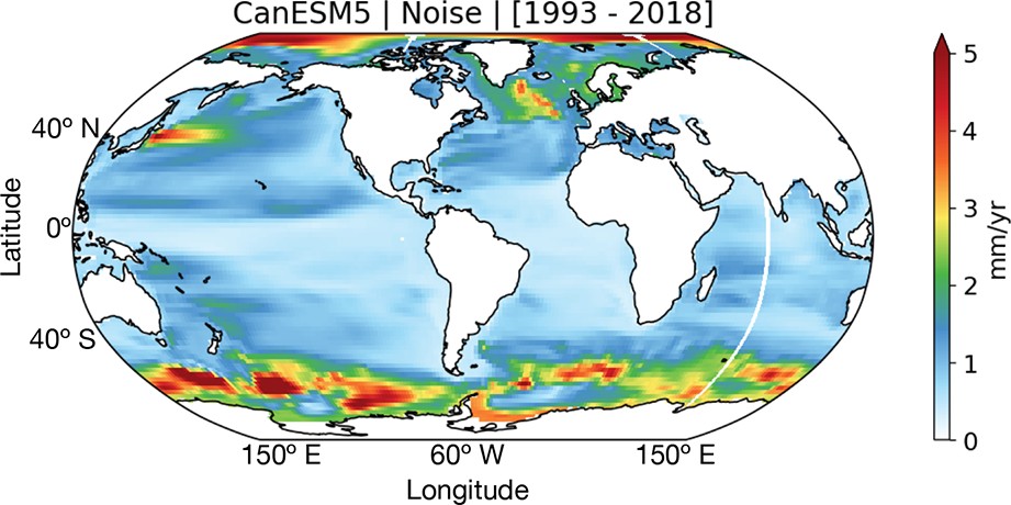
For the single-model analysis we employ the 50-member ensemble output from the Canadian Earth System Model version 5 (CanESM5, Swart et al., 2019) retrieved from the CMIP6 archive (hereafter “CanESM5 ensemble”). To compare with satellite-derived observational data, we use the historical scenario with full forcing (i.e., anthropogenic plus natural external forcings and natural internal variability, from 1850 to 2014, Fig. 1b) and the historical scenario with natural forcings only (10 members with all-natural external forcings, e.g., volcanoes, solar, but no anthropogenic emissions, from 1850 to 2020, Fig. 1c). Each historical realization starts at a different year (with 50-year intervals) from the piControl experiment, yielding differences in multidecadal ocean variability among members (Swart et al., 2019).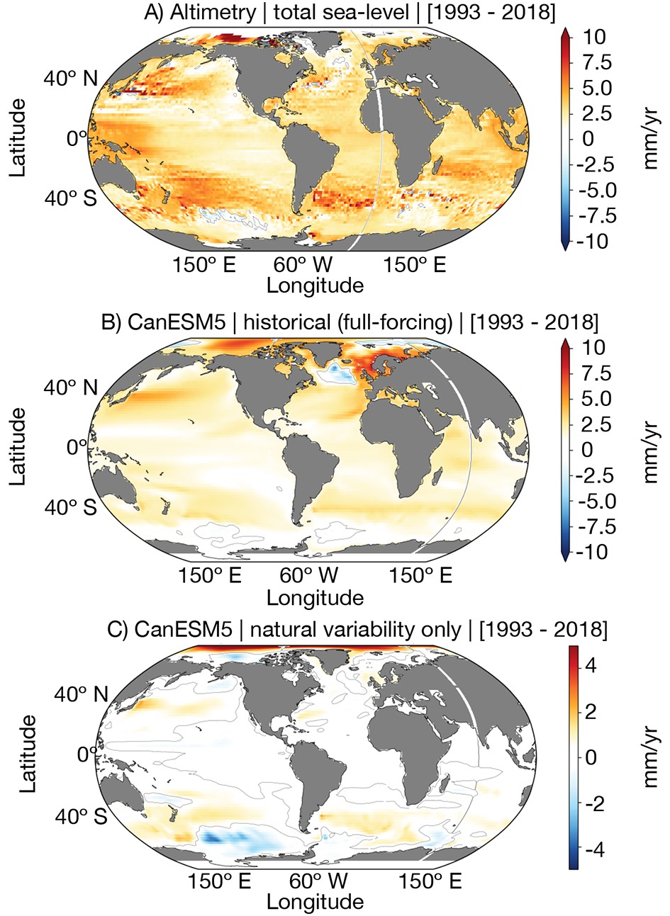 Figure1. Annual mean linear trend (mm yr?1) for the years 1993–2018 of (a) total sea level from satellite observations (AVISO+), (b) sterodynamic sea-level (DSL plus global mean thermosteric sea level) from CanESM5 historical + SSP585 (50 members average) and (c) from CanESM5 historical-natural (10 members average). The altimeter-derived sea levels refer to the ocean topography with respect to the geoid. Figure A1 in the appendix provides information about the CanESM5 intra-ensemble spread in the observed period.
There are two subset variants within this ensemble: 25 members use a conservative wind-stress field interpolation passed from the atmospheric model to the ocean model and the other 25-member subset uses a bilinear remapping scheme. These variants do not produce distinguishable responses on transient climate or global scale dynamics (Swart et al., 2019); hence, for our purposes, we can assume this to be a 50-member ensemble with the spread generated only by initial condition characteristics. The analyses were conducted using yearly means of the CanESM5 ensemble DSL results.
2
2.2. CMIP6 multi-model ensemble
The outputs from the 27 Earth System Models (ESMs) used in this study (Table 1; hereafter “CMIP6 ensemble”) are from the CMIP6 archive. The models selection was based on the availability of the DSL variable (or “zos” in CMIP convention — with zero global-area mean and not including inverse barometer depressions from sea ice) for the three “Tier 1 ScenarioMIP projections”. The model output submissions for the CMIP6 archive do not have the same number of ensemble members, so to compute our multi-model ensemble mean of the projected sea level change for the 21st century we are using a single ensemble member from each model (usually the ‘r1i1p1f1’), and every model is given the same weight for the ensemble statistics. To provide an estimate of the internal variability we are also using the last 200 years from the control run (under constant pre-industrial forcing: piControl).2
2.3. Methods
Prior to performing the CMIP6 ensemble analysis, we interpolated the DSL data from 27 different models onto a common 1° × 1° grid using bilinear interpolation with the same land–ocean mask, excluding the marginal seas and interior lakes like the Mediterranean Sea, Red Sea, Arabian Gulf, Black Sea, Caspian Sea, Baltic Sea, and Hudson Bay.Four key metrics in LE analysis were then obtained for the regional DSL data for both the CanESM5 and the CMIP6 ensemble results over the 21st century for each of the three SSPs:
(i) S — the forced response — which is the ensemble mean of the absolute linear trend in annual mean DSL spanning the period from 2015 to 2100. Trends are used to estimate sea level changes as well as other climate signals in order to highlight nonstationary behavior in the time series. This low-frequency signal can be assessed in terms of prediction, therefore providing a clearer indication of the future long-term movements in the series (Visser et al., 2015) and playing a role in climate change detection (Church et al., 2013).
(ii) N — the ensemble spread representing uncertainty – which is the standard deviation from the linear trend field among the ensemble members. Using model spread to define N should include additional model errors, whereas in the real-world N should be natural forcing and internal variability only.
(iii) S/N, as the ratio between the ensemble mean and the ensemble spread, i.e., between forced response and uncertainty.
(iv) ToE — the forced response detection time — defined as the decade over which a trend (S) will be statistically above the unforced sea level internal variability [i.e., N (Carson et al., 2019)]. Here, ToE is computed as the year when the DSL time series (with no thermosteric component) at each grid point exceeds two standard deviations of the monthly mean DSL from the piControl experiment, using the same approach as in Bordbar et al. (2015) and Lyu et al. (2014). The computation was performed for each ensemble member separately, and the resulting ToEs were averaged to obtain an ensemble mean ToE.
The CanESM5 and CMIP6 ensembles were both de-drifted using their respective piControl runs to remove potential spurious trends caused by model equilibrium adjustment rather than by external forcing. Results do not change significantly, consistent with Gupta et al. (2013), who assessed surface properties other than DSL to report that “when considering multimodel means of surface properties, drift is negligible”. The authors also investigated the steric sea level, which integrates the water column, to conclude that the deep ocean can be dominated by model drift.
The sterodynamic sea level trends (with global mean thermosteric sea level included) from 1993 to 2018 indicate good agreement between the satellite altimetry product (Fig. 1a) and the CanESM5 ensemble (Fig. 1b), both depicting major global-scale features such as the midlatitude band of positive trends. When comparing the results from both the altimetry data (Fig. 1a) and the CanESM5 full-forcing (Fig. 1b) against the CanESM5 historical-natural (Fig. 1c; note different color scale) — the latter accounting only for natural external forcings and internal variability — it can be noted that the most evident trends in Figs. 1a and b generally depart from the trends of the spatial pattern with no anthropogenic forcings (Fig. 1c). This suggests that a scenario in which only natural forcings existed would still bear the regional distribution of the full-forcing SLR scenario, albeit with much smaller magnitudes, as expected. The differences seen between the altimetry data (Fig. 1a)/CanESM5 full-forcing results (Fig. 1b) and the CanESM5 historical-natural are therefore attributable to anthropogenic external forcing.
Although sea level changes have been best explained by models driven by both natural and anthropogenic forcings, the anthropogenic forcing still seems to be the leading factor in explaining the magnitude of observed changes, while most of the variability in models seems to be caused by natural forcing, as shown by Slangen et al. (2014), when comparing full-depth observations of thermosteric sea level change to a range of single-forcing experiments done with 28 CMIP5 climate models. This study, as well as that of Marcos and Amores (2014), shows that the majority of observed global mean thermosteric sea level distribution in the second half of the 20th century is of anthropogenic origin.
Results for the future projections show common regional sea level changes relative to the global mean in both the CanESM5 and the CMIP6 ensembles (Figs. 2 and 3). The tendency to greater SLR (depicted by S) appears strongly in the Arctic (where N is also higher), the northwestern Pacific, the northern extension of the Gulf Stream, the North Indian Ocean, as well as in the northern limits of the Antarctic Circumpolar Current (ACC). In the Southern Ocean, there is a common negative change closer to the Antarctic Continent and in the southeastern Pacific.
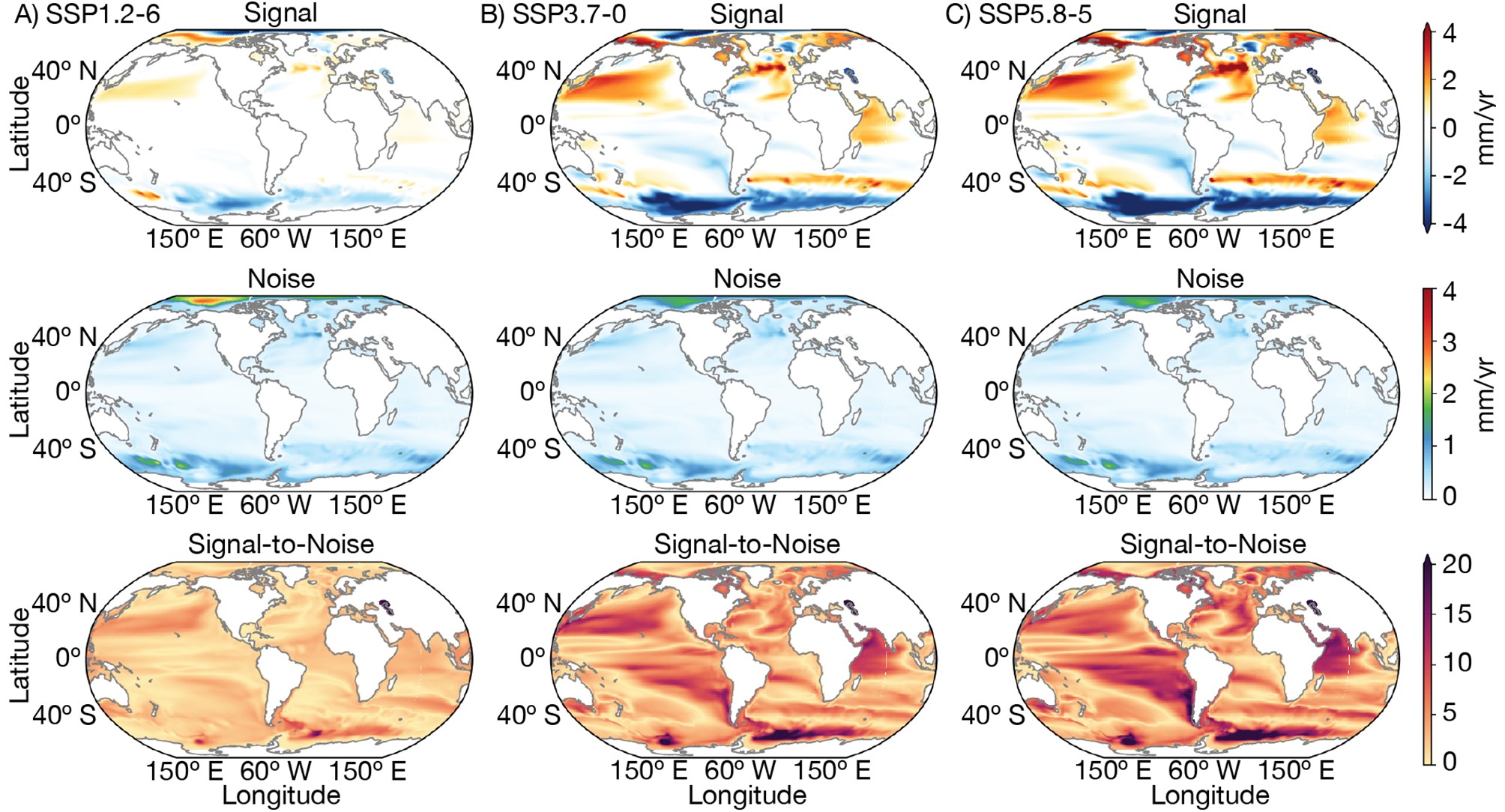 Figure2. Top: CanESM5 ensemble-mean of the linear DSL trends (mm yr?1). Middle: Spread of the ensemble trends (DSL trends’ standard deviation, mm yr?1). Bottom: The signal-to-noise ratio. The DSL trends were computed for all 50 members between 2015 and 2100 for the three SSP projections (left: SSP1-2.6; center: SSP3-7.0; right: SSP5-8.5). Figures A2 and A3 show the time series of CanESM5 global mean thermosteric sea level and local sterodynamic sea level (1850–2100) for the historical simulation and the assessed SSP scenarios.
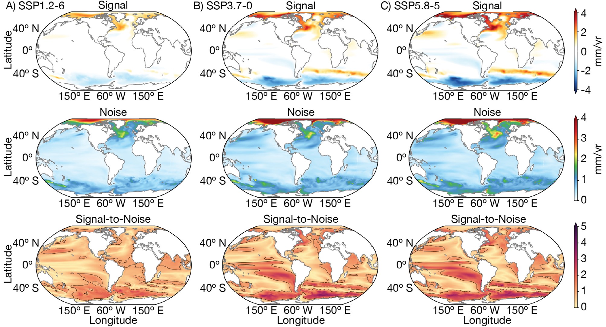 Figure3. CMIP6 multi-model mean (top) linear DSL trends (mm yr?1), spread of multi-model trends (DSL trends’ standard deviation, mm yr?1; middle), and the signal-to-noise ratio (bottom). The DSL trends were computed for all 27 models between 2015 and 2100 for the three SSP projections (left: SSP1-2.6; center: SSP3-7.0; right: SSP5-8.5).
These trends, either positive or negative, are more intense in the SSP5-8.5 scenario and display a regional distribution consistent with previous studies. Based on an ensemble of 21 CMIP5 model projections, the RCP4.5 relative regional sea level anomaly shown by Slangen et al. (2014) [e.g., Fig. 7 in Slangen et al. (2017)] is similar to the spatial patterns displayed in Figs. 2 and 3. The authors also found the highest regional sea-level changes along the North Atlantic coastal regions, and along the ACC. Features such as DSL rise in high latitudes and polar regions, as well as the Southern Ocean belt-like structure (“meridional dipole”), are also robust in CMIP3 and CMIP5 model ensembles (Yin et al., 2010; Pardaens et al., 2011; Yin, 2012; Bilbao et al., 2015). Likewise, Carson et al. (2015) found large negative sea surface height changes in the Southern Ocean, relative to the global signal.
By analyzing DSL projections from both CMIP5 and CMIP6 models, Lyu et al. (2020) concluded that they exhibit very similar features and intermodel uncertainties. Relevant improvements from CMIP5 to CMIP6 include a better representation of the location of Southern Hemisphere westerly wind stress, which in turn could be partially responsible for improving the Southern Ocean simulated mean sea level. Larger DSL changes in the North Atlantic and Arctic are also projected by CMIP6 models, which are associated with a larger weakening of the Atlantic Meridional Overturning Circulation. It is suggested that the inclusion of models with larger climate sensitivity in CMIP6, in comparison with that of the CMIP5 ensemble, might have contributed to this increase in projected DSL.
For the CanESM5 ensemble, greatest N, i.e., largest spread (Fig. 2, middle) occurs mainly at high latitudes, with values greater than 1 in the Arctic and the Southern Ocean. High values of projected DSL spread indicate an uncertainty that arises from internal climate variability. N does not vary significantly among the higher emissions projections, but is particularly larger in the Arctic for the SSP1-2.6. This suggests that the uncertainty associated with internal variability does not accompany the change in external forcing magnitude in our results, direct or indirectly. Additionally, for the CanESM5 ensemble, N is larger in regions where S is higher, suggesting that there is more uncertainty in the DSL projection over regions expected to see the biggest changes, in agreement with the results from Hu and Bates (2018) and Slangen et al. (2015).
The great advantage of using the S/N is provided by the ability to assess the significance of the DSL trends. For instance, Hu and Deser (2013) discuss that the magnitudes of the sterodynamic trends in the Southern Ocean and Arctic (2000–60) are smaller than the 95% uncertainty, and therefore statistically non-significant. Here, the magnitude (S) and spread (N) of the DSL trends are somewhat similar in the Arctic for both CanESM5 (Fig. 2) and CMIP6 (Fig. 3) results. Nonetheless, the North Atlantic dipole pattern along the Gulf Stream (North Atlantic Current) is rather clear and displays high S/N values in both ensembles for the scenarios SSP3-7.0 and SSP5-8.5 (Figs. 2 and 3), which seems to be linked to the weakening of the Meridional Overturning Circulation (Yin et al., 2009; Pardaens et al., 2011; Bouttes and Gregory, 2014; Hu and Bates, 2018). Carson et al. (2015) also reported high S/N values along the northeastern coast of the United States for results from the Max Planck Institute Earth System Model with low resolution, while the combined analysis (including CMIP5 outputs) of Carson et al. (2016) suggested that, among densely populated regions, the New York City and the northeast of North America are projected to undergo the largest changes in relative sea level during the 20th and 21st centuries.
For both the CanESM5 and CMIP6 ensembles, the regional changes projected by the SSP3-7.0 and SSP5-8.5 scenarios are fairly similar, while standing out in comparison with the changes projected by the lower-emission SSP1-2.6 (Figs. 2 and 3). This is consistent with the small differences found between the middle-RCP4.5 and the stronger-RCP8.5 forcing scenarios, by Carson et al. (2015), using 21 models from the CMIP5 archive.
In the Southern Ocean, noticeable S/N values point to high trends — more so for the SSP5-8.5 than for the SSP3-7.0 scenario, with S reaching five times the magnitude of N in the CMIP6 ensemble and up to 20 times in the CanESM5 ensemble. Forget and Ponte (2015) suggested that on long time scales wind stress variability will impact regional sea level variability across the global oceans. The stronger DSL response in the Southern Ocean has been associated with the strengthening of the westerlies (Landerer et al., 2014), which yields enhanced Ekman transport northward and intensifies the meridional sea surface height gradient. This in turn is intensified by an increased meridional temperature gradient.
Furthermore, the magnitude of this strong DSL response in the Southern Ocean could be related to surface fluxes (Clark et al., 2015). Warm sea surface temperature (SST) biases in the Southern Ocean have been reported for CMIP5 simulations (Sallée et al., 2013; Meijers, 2014) to be linked to deficiencies in atmospheric processes (Hyder et al., 2018). The same atmospheric surface flux anomalies responsible for causing the SST bias (Hyder et al., 2018) are also the source of variations in heat and freshwater fluxes as well as a poleward shift of the westerly winds (Slangen et al., 2015). Ultimately, ACC changes due to wind stress variations are possibly the main drivers of the local DSL change.
Figures 4 and 5 display the ToE for the CanESM5 and CMIP6 ensembles, respectively. The regional distribution of S/N (bottom of Figs. 2 and 3) is consistent with the spatial distribution of the decade of ToE from Figs. 4 and 5. Higher S/N can be associated with smaller uncertainties. Although the trend detection falls in similar regions for the three projections, SSP1-2.6 yields much later ToE covering a smaller area relative to the other SSPs. The CanESM5 DSL S emerges roughly two decades prior to the one of the CMIP6 ensemble, which reflects the much smaller natural forcing generated by the CanESM5 simulations, where N is a function only of initial conditions. For the CMIP6 simulations, N comes from both differences in initial conditions and also in model structure.
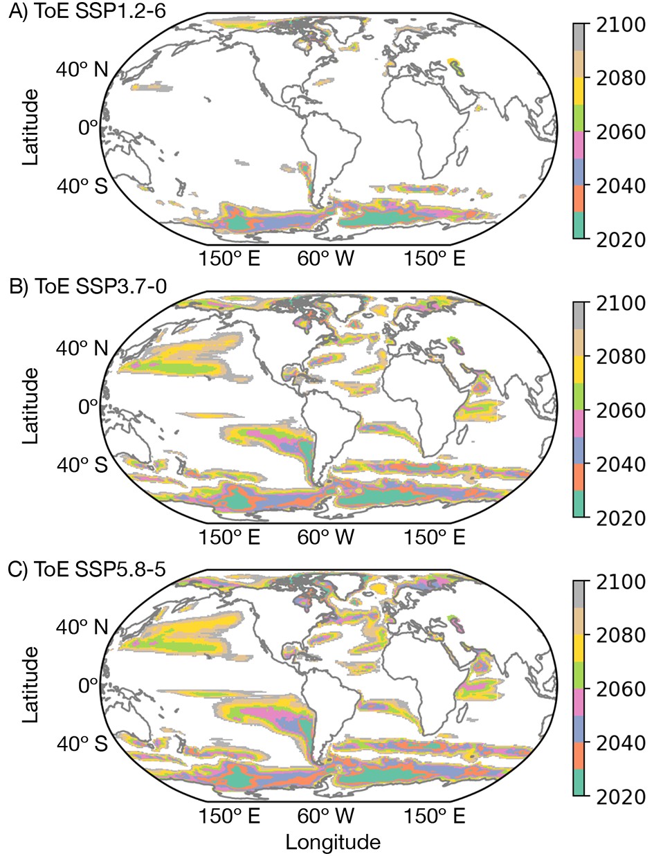 Figure4. CanESM5 ToE: Decade when the DSL time series exceeds the range of natural variability (defined by two standard deviations of the monthly mean DSL simulated in the control experiment). The illustrated ToE corresponds to the averaged ToE from all 50 members.
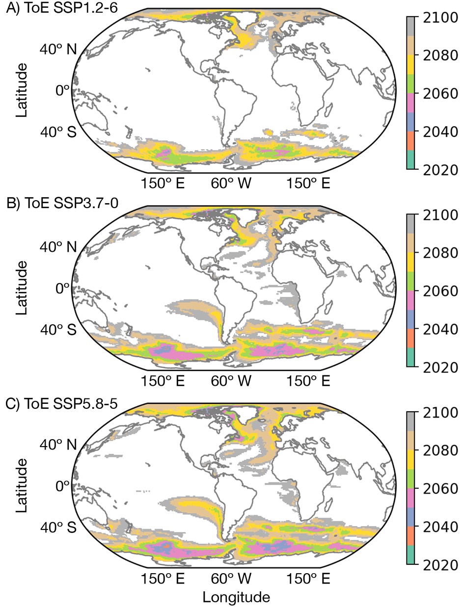 Figure5. CMIP6 ToE: Decade when the DSL time series exceeds the range of natural variability (defined by two standard deviations of the monthly mean DSL simulated in the control experiment) in each model. The illustrated ToE corresponds to the averaged ToE from all 27 models.
Although the RCP8.5-CMIP5 results from Lyu et al. (2014) show that, as a result of large internal variability, the ToE of sea-level change for DSL only (their Fig. 2a) occurs before the year of 2080 over only a small fraction of the ocean area, our CMIP6 (and also CanESM5) DSL results show ToEs occurring before 2080 over a majority of the global ocean, more in agreement with those results of Lyu et al. (2014) which consider the DSL plus the global mean thermosteric sea level (their Fig. 2b).
Although internal variability can change in response to forcing (Lehner et al., 2020), here we show that as the signal progressively increases, the DSL noise does not vary substantially across different future scenarios. It means that variations in the external forcing do not seem to significantly impact the ensembles’ spread associated with the uncertainty arising from internal climate variability (and from model differences for the CMIP6 ensemble) with respect to the DSL results analyzed here. N is reduced in the single- relative to the multi-model LE, since the latter accounts for model differences other than just internal variability. In the CanESM5 ensemble, N is larger in regions where S is higher, suggesting that there is more uncertainty in the DSL projection over regions expected to see the largest changes [in agreement with Hu and Bates (2018) and Slangen et al. (2015)].
The CanESM5 ensemble historical experiment driven by natural forcing alone cannot fully reproduce the current pattern of SLR, although its resulting regional sea level distribution resembles that of the full-forcing historical experiment, with relatively much reduced magnitudes, as expected.
The SSP3-7.0 and SSP5-8.5 scenarios project similar and equivalent DSL changes — as an adjustment to the external forcing — whereas the changes over the 21st century in the sustainable scenario (SSP1-2.6) are shown to be mostly dominated by internal variability, i.e., DSL signals remain almost entirely within the envelope of internal climate variability. This is consistent with Lyu et al. (2014), who showed that the ToE for total sea level exhibits little dependence on the emissions scenario, and occurs considerably earlier than that for the surface warming. It should be noted, however, that the total sea level variable considered by the authors also accounts for the global thermosteric mean sea level, which certainly has an emissions scenario dependence, differently from DSL.
Regional projections of sea level changes are strongly linked to global-scale processes that could exceed the range of local natural variability even in a more sustainable scenario. Nevertheless, by “Taking the Green Road” we would be approaching a reality where most of the DSL changes throughout the 21st century would be dominated by internal processes of the climate system rather than by external radiative forcing imbalance.
Acknowledgements. We acknowledge the World Climate Research Programme, which, through its Working Group on Coupled Modelling, coordinated and promoted CMIP6. We thank the climate modeling groups for producing and making available their model output, the Earth System Grid Federation (ESGF) for archiving the data and providing access, and the multiple funding agencies that support CMIP6 and ESGF. Grants CNPq-MCT-INCT-594 CRIOSFERA 573720/2008-8 and Coordenacao de Aperfeicoamento de Pessoal de Nivel Superior-Brasil (CAPES)-Finance Code 001; FAPESP 2015/50686-1; 2017/16511-5; 2018/14789-9.
 FigureA1. CanESM5 sterodynamic sea level spread (standard deviation, mm yr?1) in the observed period (1993–2018).
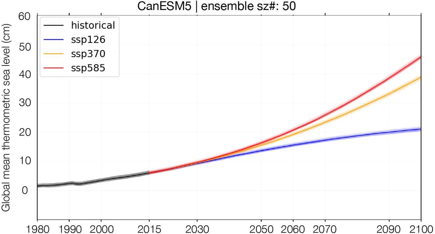 FigureA2. Time series of global mean thermosteric sea level (cm) from the CanESM5 ensemble for each SSP departing from the historical simulation. Shaded area indicates the spread for each scenario.
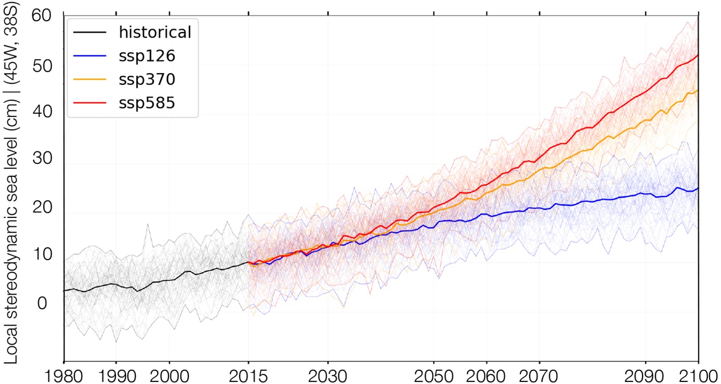 FigureA3. Time series of local (45°W, 38°S) mean sterodynamic sea level (cm) from the CanESM5 ensemble for each SSP scenario departing from the historical simulation. Thin lines indicate individual ensemble members and solid lines indicate ensemble means for each scenario.
APPENDIX
