Jozsef SZILAGYI^1,2,,,
Richard CRAGO³,
Ning MA⁴

Corresponding author: Jozsef SZILAGYI,jszilagyi1@unl.edu;

1.Department of Hydraulic and Water Resources Engineering, Budapest University of Technology H-1111, Budapest Hungary
2.Conservation and Survey Division, School of Natural Resources, University of Nebraska-Lincoln, Lincoln, Nebraska 68583, USA
3.Department of Civil and Environmental Engineering, Bucknell University, Lewisburg, Pennsylvania 17837, USA
4.Key Laboratory of Water Cycle and Related Land Surface Processes, Institute of Geographic Sciences and Natural Resources Research, Chinese Academy of Sciences, Beijing 100101, China
Manuscript received: 2020-03-23
Manuscript revised: 2020-06-18
Manuscript accepted: 2020-06-28
Abstract:Most large-scale evapotranspiration (ET) estimation methods require detailed information of land use, land cover, and/or soil type on top of various atmospheric measurements. The complementary relationship of evaporation (CR) takes advantage of the inherent dynamic feedback mechanisms found in the soil?vegetation?atmosphere interface for its estimation of ET rates without the need of such biogeophysical data. ET estimates over the conterminous United States by a new, globally calibrated, static scaling (GCR-stat) of the generalized complementary relationship (GCR) of evaporation were compared to similar estimates of an existing, calibration-free version (GCR-dyn) of the GCR that employs a temporally varying dynamic scaling. Simplified annual water balances of 327 medium and 18 large watersheds served as ground-truth ET values. With long-term monthly mean forcing, GCR-stat (also utilizing precipitation measurements) outperforms GCR-dyn as the latter cannot fully take advantage of its dynamic scaling with such data of reduced temporal variability. However, in a continuous monthly simulation, GCR-dyn is on a par with GCR-stat, and especially excels in reproducing long-term tendencies in annual catchment ET rates even though it does not require precipitation information. The same GCR-dyn estimates were also compared to similar estimates of eight other popular ET products and they generally outperform all of them. For this reason, a dynamic scaling of the GCR is recommended over a static one for modeling long-term behavior of terrestrial ET.
Keywords: land?atmosphere interactions,
land evaporation,
evapotranspiration,
complementary relationship of evaporation
摘要:区域或全球尺度的蒸散发模型大多需要翔实的土壤和植被信息作为输入。蒸散发互补原理考虑了土壤-植被-大气界面内在的动态互馈机制，故无需下垫面土壤和植被信息即可估算陆面蒸散发。本文针对前人提出的静态标度广义互补模型（GCR-stat）和作者新提出的考虑了每个时间步长陆面干湿状态的动态标度广义互补模型（GCR-dyn），利用美国大陆的327个中等流域和18个大河流域的水量平衡结果作为陆面蒸散发“实测值”，对比评估了GCR-dyn和GCR-stat的蒸散发模拟效果。结果发现，当利用多年平均的逐月驱动时，GCR-dyn模拟陆面蒸散发的效果低于GCR-stat模型，其原因是前者在多年平均尺度上不能充分利用其动态标度的优势。然而，当利用长时间尺度逐月实时驱动时，两个模型在描述蒸散发多年均值上的效果几乎一致，且即便无需降水作为输入，GCR-dyn模型在模拟蒸散发的长期变化趋势方面明显优于GCR-stat模型。进一步地与其他8个主流蒸散发产品相比较，GCR-dyn在蒸散发多年均值和长期趋势上皆具有更好的模拟效果。因此，考虑了每个时间步长陆面干湿状态的动态标度广义互补蒸散发模型优于静态标度广义互补模型，可更好地模拟地表蒸散发的长期变化特征。
关键词:地气相互作用,
陆面蒸散发,
蒸散发互补原理,

HTML

--> --> -->

Land surface evapotranspiration (ET) is a central component in the Earth’s energy, water, and carbon cycles (Wang and Dickinson, 2012; Fisher et al., 2017). Accurate ET information is therefore essential for a better understanding of land?atmosphere interactions (Seneviratne et al., 2006) and the biosphere’s water?carbon coupling (Biederman et al., 2016; Feng et al., 2016). It also improves drought predictions (Pendergrass et al., 2020) and helps to find answers to water resources sustainability issues (Condon et al., 2020). While the globally distributed eddy-covariance flux towers have contributed significantly to our knowledge of ET across a wide range of ecosystems [see a recent review by Baldocchi (2020)], the spatiotemporal variation of global ET and its response to the changing climate remains highly uncertain (Mueller et al., 2011; Liu et al., 2016) because the estimation of long-term, spatially resolved ET is yet laden by difficulties in parameterizing the biophysical processes (e.g., root water uptake, stomatal resistance and its response to CO₂ concentration changes) that control ET in the current land surface models (LSMs) (Ukkola et al., 2016; Ma et al., 2017) and remote sensing algorithms (Vinukollu et al., 2011; Velpuri et al., 2013). In addition to possible model structural errors, the uncertainties in the estimated ET can also arise from errors in their gridded vegetation (Fang et al., 2019) and soil (Zheng and Yang, 2016) parameters due to the large degree of complexity/heterogeneity found in terrestrial ecosystems. For example, most LSMs within NLDAS-2 (the North American Land Data Assimilation System, phase 2) still utilize the NOAA normalized difference vegetation index data developed by Gutman and Ignatov (1998) on a five-year-mean monthly basis without any interannual variation as input (Xia et al., 2012), failing to reasonably capture the impact of vegetation changes on ET. Besides, a recent sensitivity study by Li et al. (2018) demonstrated that the Noah-MP LSM cannot always capture the effect of spatial changes in forest and/or soil types on the simulated ET because of the inherent uncertainties in multiple land cover and soil texture data.
As an alternative, the complementary relationship (CR) (Bouchet, 1963) of evaporation inherently accounts for the dynamic feedback mechanisms found in the soil?vegetation?atmosphere interface, and thus provides a viable, robust alternative for land ET estimation relying solely on standard atmospheric forcing without the need for any soil or vegetation data. The description in the next two paragraphs of the applied CR method parallels that of Ma and Szilagyi (2019).
The generalized nonlinear version of the complementary relationship (GCR) by Brutsaert (2015) relates two scaled variables, x = E_w E_p^?1 and y = E E_p^?1 as
Here, E (mm d^?1) is the actual ET rate, while E_p (mm d^?1) is the potential ET rate, i.e., the ET rate of a plot-sized wet area in a drying (i.e., not completely wet) environment, typically specified by the Penman (1948) equation as
where $\Delta $ (hPa °C^?1) is the slope of the saturation vapor pressure curve at air temperature, T (°C), and γ is the psychrometric constant (hPa °C^?1). R_n and G are net radiation at the land surface and soil heat flux into the ground, respectively (the latter is typically negligible on a daily or longer time scale), in water equivalent of mm d^?1. The e^* term denotes the saturation, while e [= e^*(T_d)] is the actual vapor pressure of the air [hPa; their difference is called the vapor pressure deficit (VPD)]. T_d is the dewpoint temperature, and f_u is a wind function, often formulated (e.g., Brutsaert, 1982) as
where u₂ (m s^?1) is the 2-m horizontal wind speed.
The so-called wet-environment ET rate, E_w (mm d^?1), of a well-watered land surface having a regionally significant areal extent, is specified by the Priestley and Taylor (1972) equation:
The dimensionless Priestley?Taylor (PT) coefficient, α, in Eq. (4), normally attains values in the range of [1.1?1.32] (Morton, 1983). For large-scale model applications of gridded data, Szilagyi et al. (2017) proposed a method of finding a value for α, thus avoiding the need for any calibration.
Very soon after the publication of the GCR, Crago et al. (2016) and Szilagyi et al. (2017) introduced a necessary scaling into Eq. (1) by means of a time-varying wetness index, w = (E_p,max ? E_p)(E_p,max ? E_w)^?1, to define the dimensionless variable, X, as X = wx, by which Eq. (1) keeps its original nonlinear form, i.e.,
Note that Eq. (4) in Priestley and Taylor (1972) was designed with measurements under wet environmental conditions; therefore, Δ should be evaluated at the wet-environment air temperature, T_w (°C), instead of the typical drying-environment air temperature, T (Szilagyi and Jozsa, 2008; Szilagyi, 2014). By making use of a mild vertical air temperature gradient (de Vries, 1959; Szilagyi and Jozsa, 2009; Szilagyi, 2014) observable in wet environments (as R_n is consumed predominantly by the latent heat flux at the expense of the sensible one, and water representing an unusually high latent heat of the vaporization value found in nature), T_w can be approximated by the wet surface temperature, T_ws (°C). Note that T_ws may still be larger than the drying-environment air temperature, T, when the air is close to saturation, but the same is not true for T_w, due to the cooling effect of evaporation. In such cases, the estimated value of T_w should be capped by the actual air temperature, T (Szilagyi, 2014; Szilagyi and Jozsa, 2018). Szilagyi and Schepers (2014) demonstrated that T_ws is independent of the size of the wet area. Thus, T_ws can be obtained through iterations from the Bowen ratio (β) of the sensible and latent heat fluxes (Bowen, 1926) when applied over a small, plot-sized, wet patch (by the necessary assumption that the available energy for the wet patch is close to that for the drying surface) the Penman equation is valid for, i.e.,
E_p,max in the definition of X within Eq. (5) is the maximum value that E_p can achieve (under unchanging available energy for the surface) during a complete dry-out (i.e., when e becomes close to zero) of the environment, i.e.,
in which T_dry (°C) is the so-achieved dry-environment air temperature. The latter can be estimated from the (isoenthalp) adiabat of an air layer in contact with the drying surface (Szilagyi, 2018a), i.e.,
where T_wb (°C) is the wet-bulb temperature. T_wb can be obtained with the help of another iteration of writing out the Bowen ratio for adiabatic changes (e.g., Szilagyi, 2014), such as
For a graphical illustration of the saturation vapor pressure curve, the different temperatures and the related ET rates defined, please refer to Ma and Szilagyi (2019). The same source also includes a brief description of how the CR evolved into Eq. (5) over the past 40 years. Additionally, it plots selected historical CR functions over sample data, and explains how assigning a value of α is performed without resorting to any calibration. A sensitivity analysis of the ET rates in Eq. (5) to their atmospheric forcing is found in Ma et al. (2019).
While Brutsaert et al. (2020) realized the necessity of scaling x with the help of a static aridity index, Crago et al. (2016), Szilagyi et al. (2017), Szilagyi (2018a, b), Szilagyi and Jozsa (2018), Ma and Szilagyi (2019), and Ma et al. (2019) performed one (and the same one) via a dynamic wetness index. Whereas the wetness index assigns increasing values to wetter environmental conditions, the aridity index does the same to drier ones. Brutsaert et al. (2020) did not include this dynamic wetness index method in their study, and therefore the present work was initiated to fill this gap.

The time-varying (and thus dynamic) scaling of x (Crago et al., 2016; Szilagyi et al., 2017) by the wetness index, w [= (E_p,max ? E_p)(E_p,max ? E_w)^?1], in Eq. (5), is necessary because the GCR of Brutsaert (2015) unrealistically predicts near-zero land evaporation only when E_w in x itself approaches zero. This is because the potential evaporation rate, E_p, in the denominator of x always assumes well-bounded values due to physical limits on the range of its constituents, i.e., net radiation, soil heat flux, air temperature, wind speed, and VPD.
An alternative, static scaling of x by Brutsaert et al. (2020) takes place via an adjustable parameter, α_c, that acts as the PT-α value for wet environments. Since Eq. (4) can also be written as E_w = αE_e, where E_e is the equilibrium evaporation rate of Slatyer and Mcllroy (1961), thus the scaled variable, X, becomes X = α_c E_e E_p^?1 = α_cxα^?1. The spatially variable (but constant through time at a given location) value of α_c was then related to a long-term aridity index by Brutsaert et al. (2020), with the latter defined as the ratio of the mean annual E_p and rain depth, and globally calibrated with the help of additional water-balance data, requiring altogether seven parameters in highly nonlinear equations.
Note that the X = wx scaling by Crago et al. (2016) and Szilagyi et al. (2017) requires only the forcing variables (R_n, G, T, u₂, and VPD), without the need for external precipitation/rain data, which is significant as precipitation is possibly the most uncertain meteorological variable to predict in climate models. It is important to mention that w changes with each value of x, unlike α_c. As Szilagyi et al. (2017) demonstrated, a (temporally and spatially) constant value of the PT α, necessary for x, can be set by the sole use of the forcing variables, without resorting to additional water-balance data of precipitation and stream discharge, thus making the approach calibration-free on a large scale (Szilagyi, 2018b; Ma et al., 2019; Ma and Szilagyi, 2019) where wet-environmental conditions, necessary for setting the value of α, can likely be found. Note that setting a constant value of α is also necessary for Brutsaert et al. (2020) in order to force their spatially variable but temporally constant α_c values to reach a predetermined value of about 1.3 under wet conditions. Despite almost half a century of research following publication of the Priestley and Taylor (1972) equation, there is still no consensus about what environmental variables (atmospheric, radiative, and/or surficial properties), and exactly how their spatial and temporal averaging, influence the value of the PT α. Until compelling information is available on these variables, a spatially and temporally constant α value may suffice for modeling purposes.
As was found by Szilagyi (2018b), the value of the PT α depends slightly on the temporal averaging of the forcing data, i.e., whether or not the monthly values are long-term averages [yielding α = 1.13 (Szilagyi et al., 2017) and 1.15 (Szilagyi, 2018b), respectively]. Therefore, here, it is tested if such is the case for the globally calibrated model of Brutsaert et al. (2020). Namely, if its performance is affected by similar changes (from long-term mean monthly values to monthly values) in the input/forcing variables, then some caution must be exercised during its routine future application, and recalibration of its seven parameters may be necessary. Note that besides the different scaling of x, everything is the same (including data requirements) in the two GCR model versions applied here, except that Δ in E_e is evaluated at the measured air temperature in Brutsaert et al. (2020) while the same in E_w (= αE_e) is evaluated at an estimated wet-environment air temperature (Szilagyi et al., 2017) explained above.
Both model versions (denoted for brevity by GCR-stat and GCR-dyn, respectively) were tested over the conterminous United States, first with long-term averages (1981?2010) of monthly 32-km resolution North American Regional Reanalysis (NARR) (Mesinger et al., 2006) radiation and 10-m wind (u₁₀) data [reduced to 2-m values via u₂ = u₁₀ (2/10)^1/7 (Brutsaert, 1982)], as well as with 4.2-km PRISM air, and dewpoint temperature values (Daly et al., 1994) followed by a continuous 37-year simulation of monthly values over the 1979?2015 period. The NARR data were resampled to the PRISM grid by the nearest neighbor method. Monthly soil heat fluxes were considered negligible. Evaluation of the model estimates were performed by water-balance estimates of basin-representative evaporation rates (E_wb) with the help of United States Geological Survey two- and six-digit Hydrologic Unit Code (HUC2 and HUC6) basin (Fig. 1) discharge data (Q) together with basin-averaged PRISM precipitation (P) values as E_wb = P ? Q, either on an annual (for trend analysis) or long-term mean annual basis. The application of a simplified water balance is justifiable as soil-moisture and groundwater-storage changes are typically negligible over an annual (or longer) scale (Senay et al., 2011) for catchments with no significant trend in the groundwater-table elevation values.
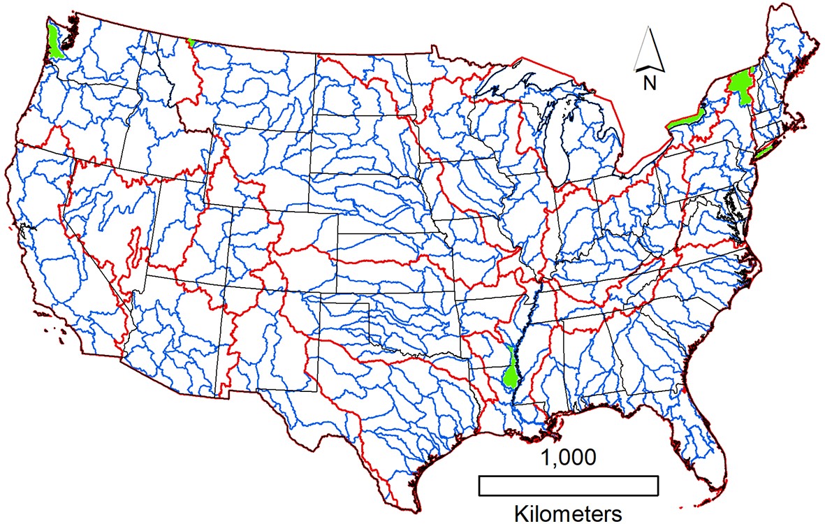Figure1. Distribution of the 18 HUC2 (outlined in red) and 334 HUC6 basins across the conterminous United States. Seven HUC6 basins, marked by green, yielded outlying water-balance-derived evaporation estimates and were left out of model comparisons.

With the long-term mean monthly data, GCR-stat performed slightly but consistently better than GCR-dyn (Fig. 2), reflected best in the Nash?Sutcliffe model efficiency (NSE) and root-mean-square error (RMSE) values, both models providing unbiased, basin-averaged mean annual ET estimates. This outcome is unsurprising, as GCR-stat takes advantage of measured precipitation while GCR-dyn does not.
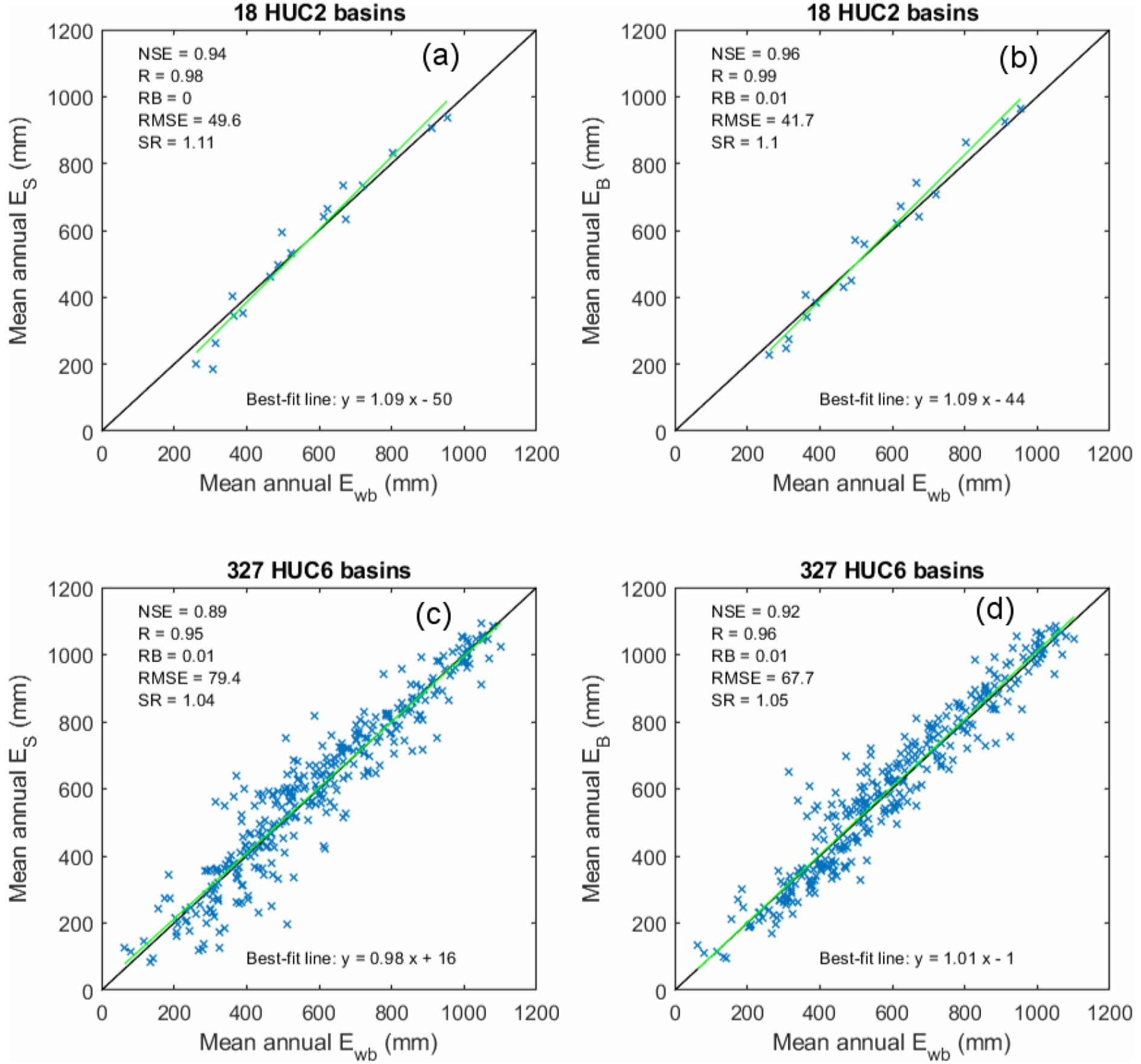Figure2. Regression plots of model estimates [E_S (a, c) from GCR-dyn; E_B (b, d) from GCR-stat) against water-balance (E_wb) evaporation rates. Long-term mean (1981?2010) monthly values served as model forcing. α = 1.13 in GCR-dyn (a, c). NSE: Nash?Sutcliffe model efficiency; R: linear correlation coefficient; RB: relative bias; RMSE: root-mean-square error (mm); SR: ratio of standard deviations of the mean annual model and water-balance values.


However, the picture changes when switching from long-term mean monthly forcing values to monthly values in a continuous simulation (Fig. 3). GCR-dyn, with a slightly changed PT-α value [from 1.13 to 1.15, using the procedure of Szilagyi et al. (2017)] continues to produce unbiased estimates of basin-averaged mean annual evaporation values. However, the globally calibrated GCR-stat model underestimates the water-balance-derived values by about 10% [i.e., relative bias (RB) of ?0.09 for both basin scales] and produces reduced interannual variability (see the horizontally elongated “crosses” for the HUC2 basins in Fig. 3) in comparison with GCR-dyn. Reduced model performance of GCR-stat is also apparent in the long-term linear tendencies (obtained as least-squares fitted linear trends) of the basin-averaged annual evaporation values (Fig. 4) by being less effective than GCR-dyn in reproducing the observed linear trends in the water-balance data.
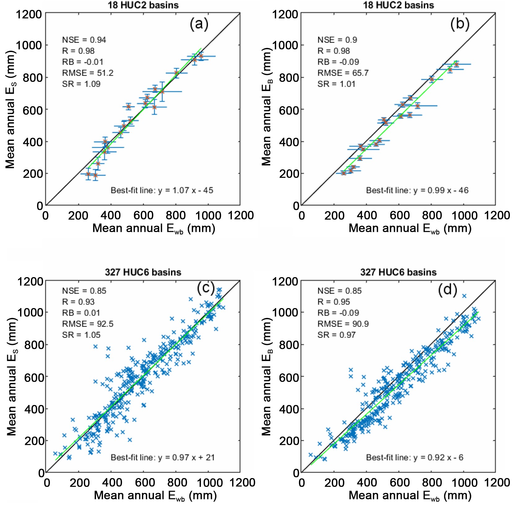Figure3. Regression plots of model estimates [E_S (a, c) from GCR-dyn; E_B (b, d) from GCR-stat] against water-balance (E_wb) evaporation rates. Monthly (1979?2015) values served as model forcing for the continuous simulation of monthly evaporation rates. α = 1.15 in GCR-dyn (a, c). The vertical and horizontal bars represent the standard deviation of the annual modeled and water-balance HUC2 values, respectively. The large number of data points hinders a similar plot for the HUC6 values.


Figure4. Regression plots of the linear trends (1979?2015) in annual modeled [E_S (a, c) from GCR-dyn; E_B (b, d) from GCR-stat] and water-balance values. The vertical and horizontal bars represent the standard error in the trend-value estimates for the modeled and water-balance HUC2 values (a, b), respectively. The large number of data points hinders a similar plot of the HUC6 values (c, d). RMSE is now in mm yr^?1.


As on a mean-annual basis GCR-stat performs better than (with mean monthly values) or about equal to (in a continuous simulation) GCR-dyn by exploiting precipitation data (which on the watershed scale naturally serves as an upper bound for land ET), its weakened performance in trends can only be explained by the same reliance on the long-term means of the precipitation (and E_p) rates in the (therefore) static α_c values that will hinder its response to slow (decadal) changes in aridity. The same problem cannot occur in GCR-dyn, since its wetness index (w) is updated in each step of calculations.
The current GCR-dyn model has already been shown to (a) yield correlation coefficient values in excess of 0.9 with local measurements of latent heat fluxes across diverse climates in China (Ma et al., 2019) in spite of large differences in spatial representativeness (i.e., grid resolution vs flux measurement footprint), and (b) outperform several popular large-scale ET products over the conterminous United States (Ma and Szilagyi, 2019). These products include three LSMs—namely, Noah (Chen and Dudhia, 2001), VIC (Liang et al., 1994), and Mosaic (Koster and Suarez, 1996); two reanalysis products—namely, NCEP-II (Kanamitsu et al., 2002), and ERA-Interim (Dee et al., 2011); another two remote-sensing based approaches—namely, GLEAM (Miralles et al., 2011; Martens et al., 2017) and PML (Zhang et al., 2017; Leuning et al., 2008); and a spatially upscaled eddy-covariance measurement product, FLUXNET-MTE (Jung et al., 2011). In a comparison with water-balance data, GCR-dyn turns out to produce even better statistics on the HUC2 scale than the spatially interpolated eddy-covariance measured ET fluxes (Fig. 5), which is remarkable from a calibration-free approach. GCR-dyn especially excels in the long-term linear tendency estimates of the HUC2 ET rates, demonstrated by Figs. 6 and 7. As FLUXNET-MTE employs several temporally static variables for its spatial interpolation method, its ability to capture long-term trends is somewhat limited (Jung et al., 2011). On the contrary, the dynamic scaling inherent in GCR-dyn automatically adapts to such trends and identifies them rather accurately.
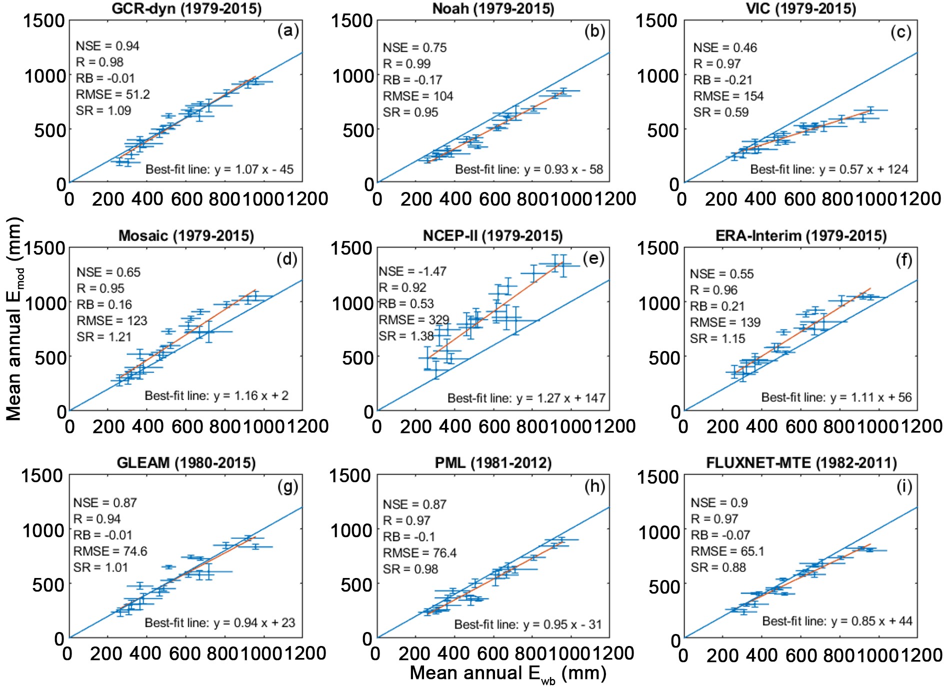Figure5. Regression plots of the HUC2-averaged multiyear mean annual ET rates (E_mod) of GCR-dyn (a) and eight other (b?i) popular large-scale ET models against the simplified water-balance (E_wb) estimates. Temporal averaging follows the availability of data displayed in parentheses for each product. The length of the whiskers denotes the standard deviation of the HUC2-basin averaged annual ET values. The long blue line represents a 1:1 relationship, while the least-squares fitted linear relationships are shown in maroon color (after Ma and Szilagyi, 2019).


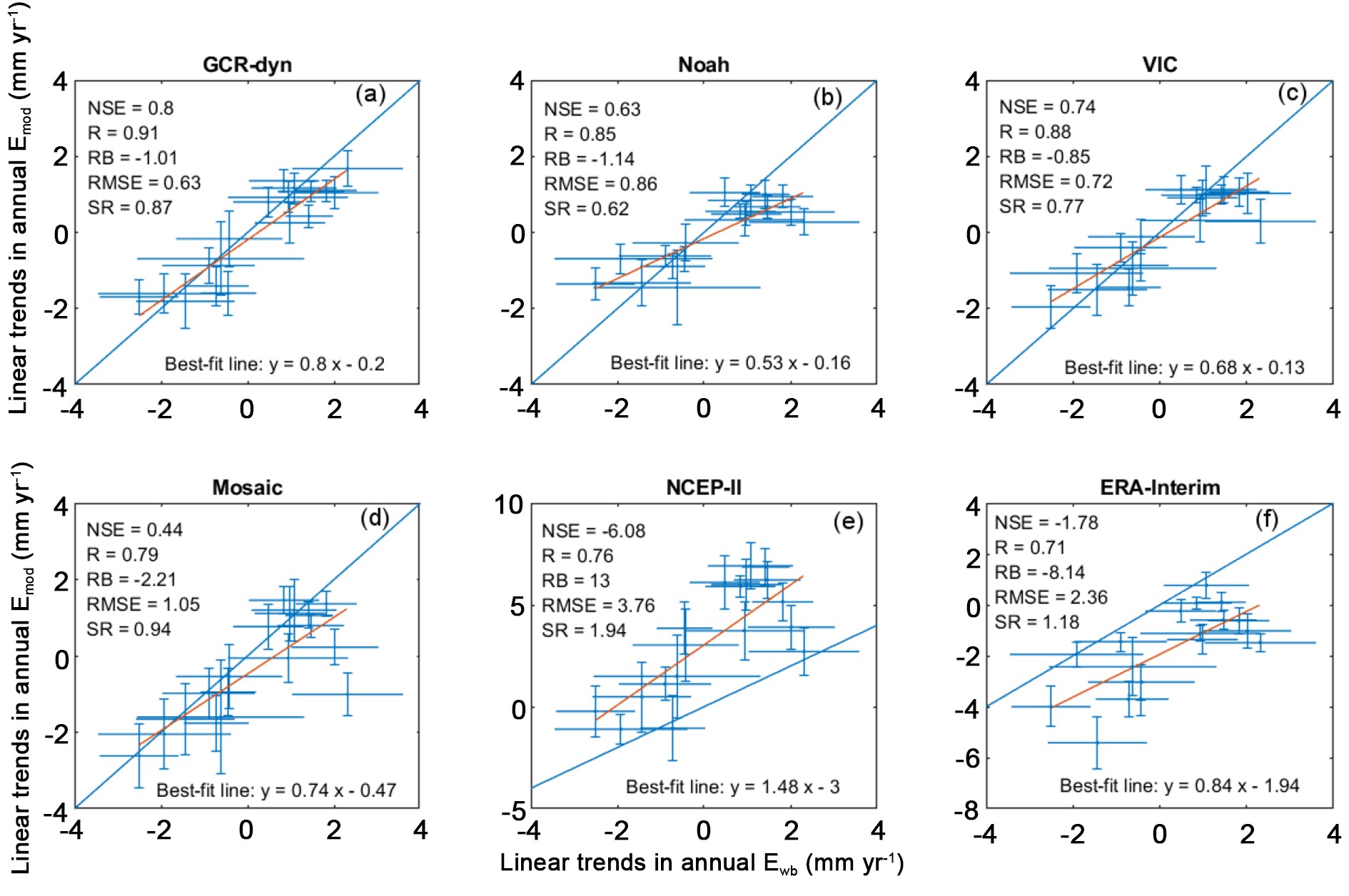Figure6. Regression plots of the linear trend values (mm yr^?1) in modeled HUC2-averaged annual ET sums (E_mod) against those in E_wb over 1979?2015. The length of the whiskers denotes the standard error in the estimated slope value. The long blue line represents a 1:1 relationship, while the least-squares fitted linear relationships are shown in maroon color (after Ma and Szilagyi, 2019).


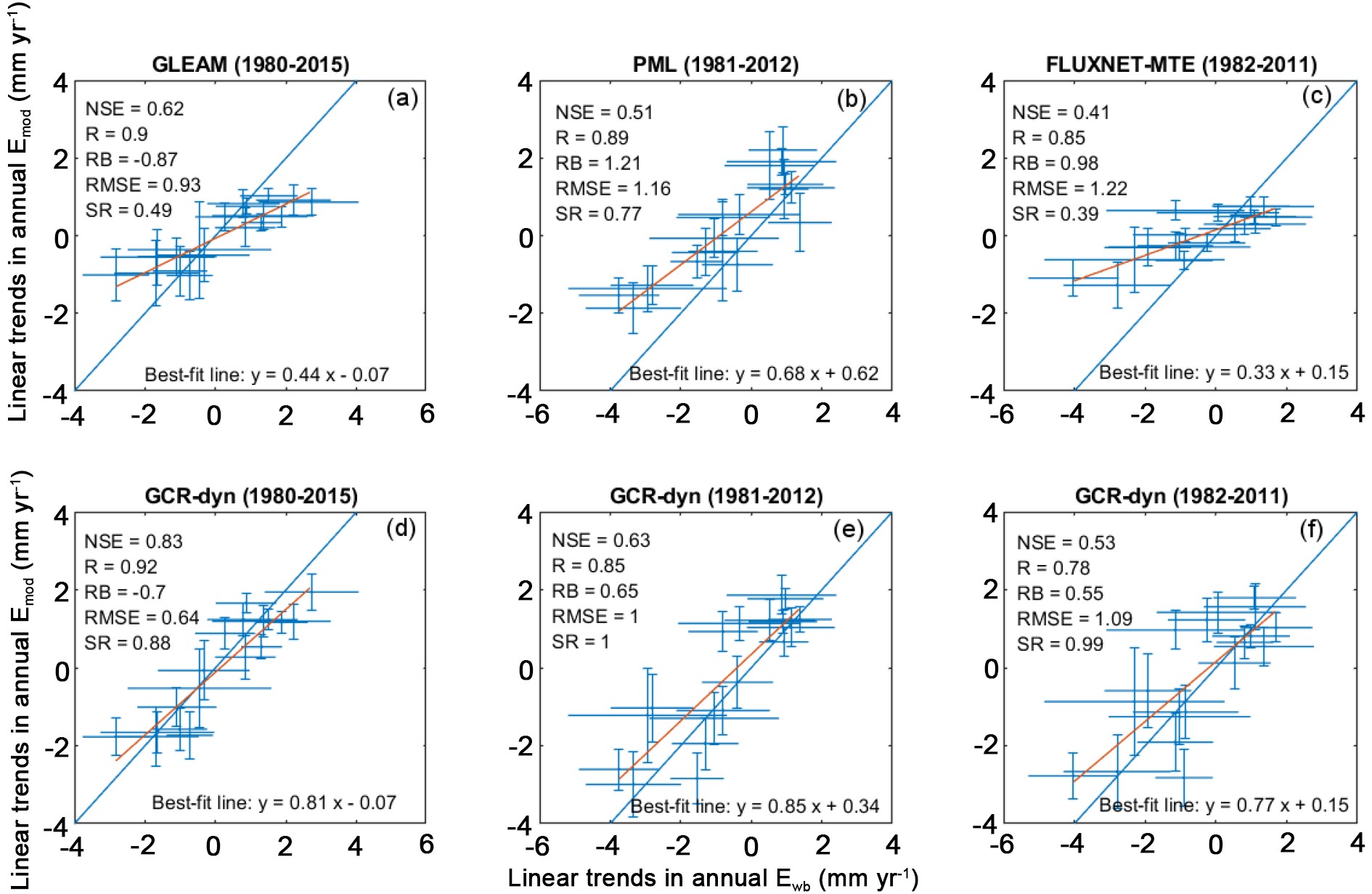Figure7. Regression plots of the linear trend values (mm yr^?1) in GLEAM-, PML-, and FLUXNET-MTE-modeled (a?c) HUC2-averaged annual ET sums (E_mod) against those in E_wb over the different model periods (shown in parentheses). For comparison, regressions for the GCR-dyn ET values over the same periods are also displayed (d?f). The length of the whiskers denotes the standard error in the estimated slope value. The long blue line represents a 1:1 relationship, while the least-squares fitted linear relationships are shown in maroon color (after Ma and Szilagyi, 2019).


Among the different popular large-scale ET models, GCR-dyn produces multi-year mean annual ET rates closest in its spatial distribution to those of FLUXNET-MTE (Fig. 8), with a spatially averaged ET value almost identical (both in its spatial average and standard deviation) to that of GLEAM (Fig. 8), which is a remote-sensing based approach. Note that all models of the comparison (except GCR-dyn) rely on precipitation data as input, which greatly aids ET estimations, as on a regional scale and long-term basis precipitation forms an upper bound for terrestrial ET rates; plus, it may drive any required soil-moisture water-balance calculations.
Figure8. Spatial distribution of the multiyear (1979?2015) mean annual ET (mm) rates (E_mod) by GCR-dyn and eight other popular large-scale ET models (a?i) and their spatially averaged (j) values, plus/minus standard deviations (after Ma and Szilagyi, 2019). The 18 HUC2 basins are also outlined.


The spatial distribution of the modeled multi-year linear ET trends is displayed in Fig. 9. Again, GCR-dyn produces results closest in spatial distribution to FLUXNET-MTE in terms of the statistically significant trends and to GLEAM in general. For a more detailed discussion of model comparisons (including additional model descriptions), please refer to Ma and Szilagyi (2019).
Figure9. Spatial distribution of the linear tendencies (mm yr^?1) in annual ET sums of GCR-dyn and eight other popular large-scale ET products. The stippling denotes trends that are statistically significant (p < 5%) in the Student’s t-test (after Ma and Szilagyi, 2019).


In conclusion, it can be stated that the GCR of evaporation (Brutsaert, 2015) is a very effective tool in land ET modeling, as it requires only a few, largely meteorological forcing variables, and avoids the need for detailed soil-moisture and land-cover information. Although attractive, as its (altogether seven) parameters have already been globally precalibrated, the GCR model version (GCR-stat) of Brutsaert et al. (2020) may, however, not perform optimally in estimating long-term tendencies in basin-wide ET rates. This is particularly the case in comparison to an earlier, calibration-free version (GCR-dyn), having no precalibrated parameter values but requiring that its sole, temporally?and spatially?constant parameter (i.e., the PT coefficient) be set using the actual forcing data through a largely automated method, described in Szilagyi et al. (2017). Since in a continuous monthly simulation both models performed about the same, while the GCR-dyn produced better long-term tendencies, a dynamic scaling of E_w E_p^?1 is recommended over a static one in future applications of the GCR of evaporation.
As has been recommended before (Szilagyi, 2018b; Szilagyi and Jozsa, 2018; Ma and Szilagyi, 2019), it is reiterated here that GCR-dyn, due to its minimal data requirement, calibration-free nature and dynamic scaling, may continue to serve as a diagnostic and benchmarking tool for more complex and data-intensive models of terrestrial ET rates, including calibration/verification (for past values) and reality checking (for future scenario values) of the LSM-predicted ET rates of existing regional and general circulation models.
Acknowledgements. All data used in this study can be accessed from the following websites. NARR data: www.esrl.noaa.gov/psd/data/gridded/data.narr.html. PRISM temperature, humidity and precipitation: prism.oregonstate.edu/. USGS HUC2 and HUC6 runoff: waterwatch.usgs.gov /?id=wwds_runoff. Noah ET data: disc.gsfc.nasa.gov/datasets/NLDAS_NOAH0125_M_V002/summary?keywords=NLDAS. VIC ET data: disc.gsfc.xnasa.gov/datasets/NLDAS_VIC0125_M_V002/summary?keywords=NLDAS. Mosaic ET data: disc.gsfc.nasa.gov/datasets/NLDAS_ MOS0125_M_V002/summary?keywords=NLDAS. NCEP-II ET data: www.esrl.noaa.gov/psd/data/gridded/data.ncep.reanalysis2.html. ERA-Interim ET data: www.ecmwf.int/en/forecasts/datasets/reanalysis-datasets/era-interim. GLEAM ET data: http://gleam.eu/#home. PML ET data: data.csiro.au/dap/landingpage?pid=csiro:17375&v= %202&d=true. FLUXNET-MTE ET data: climatedataguide.ucar.edu/climate-data/fluxnet-mte-multi-tree-ensemble. The GCR-dyn modeled ET rates and the HUC2- and HUC6-averaged E_wb, P, Q, data are available from https://digitalcommons.unl.edu/natrespapers/986/. This research was supported by a BME-Water Sciences and Disaster Prevention FIKP grant of EMMI (BME FIKP-VIZ).
Open Access This article is distributed under the terms of the creative commons attribution 4.0 international license (http://creativecommons.org/licenses/by/4.0/), which permits unrestricted use, distribution, and reproduction in any medium, provided you give appropriate credit to the original author(s) and the source, provide a link to the creative commons license, and indicate if changes were made.