Qingchang QIN^1,2,6,
Xueshun SHEN²,
Chungang CHEN³,
Feng XIAO⁴,
Yongjiu DAI⁵,
Xingliang LI^2,,

Corresponding author: Xingliang LI,lixliang@cma.cn

1.College of Global Change and Earth System Science, Beijing Normal University, Beijing 100875, China
2.Center of Numerical Weather Predication, China Meteorological Administration, Beijing 100081, China
3.State Key Laboratory for Strength and Vibration of Mechanical Structures, Xi’an Jiaotong University, Xi’an 710049, China
4.Department of Mechanical Engineering, Tokyo Institute of Technology, Tokyo 226-8502, Japan
5.School of Atmospheric Sciences, Sun Yat-Sen University, Guangzhou 510275, China
6.Beijing Meteorological Observatory, Beijing 100089, China
Manuscript received: 2019-01-02
Manuscript revised: 2019-04-19
Manuscript accepted: 2019-05-13
Abstract:A 3D compressible nonhydrostatic dynamic core based on a three-point multi-moment constrained finite-volume (MCV) method is developed by extending the previous 2D nonhydrostatic atmospheric dynamics to 3D on a terrain-following grid. The MCV algorithm defines two types of moments: the point-wise value (PV) and the volume-integrated average (VIA). The unknowns (PV values) are defined at the solution points within each cell and are updated through the time evolution formulations derived from the governing equations. Rigorous numerical conservation is ensured by a constraint on the VIA moment through the flux form formulation. The 3D atmospheric dynamic core reported in this paper is based on a three-point MCV method and has some advantages in comparison with other existing methods, such as uniform third-order accuracy, a compact stencil, and algorithmic simplicity. To check the performance of the 3D nonhydrostatic dynamic core, various benchmark test cases are performed. All the numerical results show that the present dynamic core is very competitive when compared to other existing advanced models, and thus lays the foundation for further developing global atmospheric models in the near future.
Keywords: multi-moment constrained finite-volume method,
nonhydrostatic,
dynamic core,
topography,
height-based terrain-following coordinate
摘要:在原来二维非静力大气模式框架基础上，本文采用3点多矩约束有限体积格式发展了一个含地形的三维完全可压缩非静力有限体积大气模式动力框架。多矩约束有限体积方法定义了两类矩：（1）点值（PV矩），（2）体积积分平均值（VIA矩）。通过大气控制方程，单元网格内未知变量（即PV矩）的时间演变得以更新；而积分平均值（VIA矩）通过有限体积通量形式方法更新其时间演变，进而保证了数值的严格守恒。与现有的其他方法相比，本文发展的三维大气模式框架所采用的3点多矩约束有限体积算法，具有一致的3阶精度、模板紧致和算法简洁等优势。为了检验发展的三维大气模式框架性能，本文进行了各种标准数值测试包括陡峭地形数值测试，数值模拟结果表明新发展的三维大气模式框架可与现有的先进大气模式相媲美。本研究为进一步发展全球多矩约束有限体积模式奠定基础。
关键词:多矩约束有限体积法,
非静力,
模式动力框架,
地形,
高度地形追随坐标

HTML

--> --> -->

With the rapid development of computational power, it is possible for numerical weather prediction models to simulate smaller scales of flows with finer resolution. With the resolution of the models increased, nonhydrostatic effects become very important. In recent decades, many nonhydrostatic formulations have been investigated; and today, almost all limited-area models (Benoit et al., 1997; Hodur, 1997; Doms and Sch?ttler, 1999; Xue et al., 2000; Chen et al., 2008; Skamarock and Klemp, 2008) use a nonhydrostatic dynamic core. In order to take full advantage of computers with massive cores, researchers should pay more attention to the underlying numerical algorithms of their models. The numerical methods designed should be local in nature, which implies a lower cost of communication (Dennis et al., 2012). Local high-order schemes such as the spectral element methods (Patera, 1984; Thomas and Loft, 2000; Iskandarani et al., 2002; Fournier et al., 2004; Giraldo and Rosmond, 2004; Karniadakis and Sherwin, 2005; Taylor and Fournier, 2010) and discontinuous Galerkin methods (Cockburn and Shu, 1998; Levy et al., 2007; Giraldo and Restelli, 2008; Hesthaven and Warburton, 2008; Nair et al., 2009; Restelli and Giraldo, 2009; Blaise and St-Cyr, 2012) possess all of these characteristics and have been widely used in geophysical fluid dynamics. But, these high-order schemes are more computationally expensive, and must follow a restrictive Courant?Friedrichs?Lewy (CFL) condition for the maintenance of computational stability (Zhang and Shu, 2005).
Recently, another type of high-order scheme with local reconstructions, the so-called multi-moment constrained finite-volume method (MCV), has been developed (Ii and Xiao, 2009). The basic idea of this method is the multi-moment concept (Yabe and Aoki, 1991; Yabe et al., 2001; Xiao, 2004; Ii et al., 2005; Xiao et al., 2005, 2006; Xiao and Ii, 2007), where we make use of different kinds of discrete quantities, such as the point-wise value (PV), the volume-integrated average (VIA), and the derivatives of different orders, which are called “moments” in our context, to describe physical fields. With these moments locally defined, high-order reconstructions can be built in compact stencils. Instead of updating the moments directly (Chen and Xiao, 2008; Li et al., 2008; Akoh et al., 2010), the MCV formulation updates values at the points as the basic model variables located in each mesh element (Li et al., 2013b). The values at solution points are predicted by time evolution equations obtained from imposing a set of constrained conditions on different types of moments. In the MCV method, some constraint conditions are applied on the boundaries of the computational element, where the derivatives of the numerical flux are solved as derivative Riemann problems.
In comparison with other existing high-order schemes, the MCV method allows a less restrictive CFL condition for computational stability (Ii and Xiao, 2009). Besides, an MCV model has exact numerical conservation through a constraint on the VIA moment and shows superiority in computational efficiency and algorithmic simplicity. So far, this method has been successfully implemented to develop 2D global advection and shallow models on different grids (Ii and Xiao, 2010; Chen et al., 2012; Li et al., 2012; Li et al., 2013a; Chen et al., 2014a, b; Xie and Xiao, 2016), as well as a nonhydrostatic dynamic core on a Cartesian grid (Li et al., 2013b, 2016), which has been demonstrated as a robust high-order method for a new type of numerical framework. Zhang et al. (2017) also showed that the MCV method has good scalability on high-performance computers, thus allowing massively parallel computing with thousands of process cores.
In this paper, given the attractive results of the previous 2D three-point MCV nonhydrostatic atmospheric dynamics (Li et al., 2013b), we further extend it to a 3D nonhydrostatic dynamic core and verify its performance, which will set the stage for the development of practical global atmospheric modeling. The remainder of the paper is organized as follows: In section 2, the 3D governing equations with the effect of topography are described in detail. The basic numerical formulation of the three-point MCV scheme follows in section 3. Numerical results from benchmark tests are presented in section 4. And finally, a short conclusion is given in section 5.

The nonhydrostatic atmospheric governing equations can be written in different forms (Giraldo and Restelli, 2008). Here, we utilize the following form:
where ρ is the air density; V = (u, v, w)^T is the 3D velocity field in the Cartesian coordinate; f is the Coriolis parameter; and θ is the potential temperature, which is related to the air temperature T and pressure p by $\theta = T{({{{p_0}}/p})^{{R_d}/{c_p}}}$. The continuity equation, Eq. (1), enforces the conservation of mass, and the equation of potential temperature, Eq. (5), enforces the conservation of entropy. Equations (2)?(4) enforce momentum conservation without the source terms. In order to close the above system, the equation of state is expressed by $p = {C_0}{(\rho \theta)^\gamma }$, where ${C_0} = {R_d}^\gamma {p_0}^{ - {R_d}/{c_v}}$. The constants used in the above relations are given as follows: p₀ = 10⁵ Pa is the reference surface pressure; c_p = 1004.5 J kg^?1 K^?1 represents specific heat capacity of dry air at constant pressure and c_v = 717.5 J kg^?1 K^?1 is the specific heat capacity of dry air at constant volume; γ = c_p/c_v = 1.4 is the ratio of specific heats; R_d = 287 J kg^?1 K^?1 is the ideal gas constant of dry air; and g = 9.806 16 m s^?2 is the gravitational acceleration.

2

-->

2.1. Splitting of reference profile

As generally used in atmospheric modeling, thermodynamic variables are written as the sum of the mean state and perturbation (Skamarock and Klemp, 2008):
where the mean state (denoted by the overbar) satisfies local hydrostatic balance:
Under this splitting, Eqs. (1)?(5) take the form
where $p' = {\varepsilon _0}(\rho \theta)',\;{\varepsilon _0} = \gamma {C_0}{(\overline {\rho \theta })^{\gamma - 1}}$. It should be noted that the present core is targeted to short-term weather prediction, so that the mean state can be reasonably determined based on the current conditions of the atmosphere.

2 -->

2.2. Incorporation of topography

Owing to the advantages of accuracy and flexibility, a terrain-following height-based coordinate is preferred in many nonhydrostatic models (Prusa et al., 2008; Skamarock et al., 2012), as originally proposed by Gal-Chen and Somerville (1975). Here, we use a more sophisticated terrain-following coordinate system (Sch?r et al., 2002) to map the Cartesian space (x, y, z) to computational space (x, y, ζ)
where h is the topographic height, H is the altitude of the model top, and s is the scale height parameter.
The coordinate transformation enters the governing equations through the metric coefficients G_1,3 and G_2,3, and the Jacobian of the transformation $\sqrt G $. Following standard notation (Clark, 1977), they are defined as
For an arbitrary field variable ?, the following chain rules (Clark, 1977) connecting the (x, y, z) with the (x, y, ζ) coordinate system are used:
Thus, the divergence operator of a flux F = (F_x, F_y, F_z) takes the following form:
The vertical velocity in the transformed coordinate is

2 -->

2.3. Governing equations

Substituting the relations of Eqs. (16)?(21) into Eqs. (10)?(14), the governing equations in the transformed coordinate are written as follows:
We rewrite Eqs. (22)?(26) into the following vector form:
where ${{q}} = {\left[ {\sqrt G \rho ',\sqrt G \rho u,\sqrt G \rho v,\sqrt G \rho w,\sqrt G (\rho \theta)'} \right]^{\rm{T}}}$ is the state vector; ${{{s_{\rm{st}}}}}{\rm{(}}{{q}}{\rm{)}}\;{\rm{ = }}\;{\left[ {0,f\rho v, - f\rho u, - \rho 'g,0} \right]^{\rm{T}}}$ represents the source terms; and
and
are the flux vectors in the x, y and ζ directions, respectively.

2 -->

2.4. Eigenvalues and eigenvectors of the governing equations

As in section 3, the eigenvalues and eigenvectors of the hyperbolic parts of the governing equations are needed when we compute the derivative Riemann problems. For convenience, we briefly discuss how to calculate them here. Considering the homogeneous part of the governing equations, Eqs. (22)?(26), the set of hyperbolic equations in 3D is given as follows:
The linearized form of Eq. (28) is written as
where A, B and C are the Jacobian matrices corresponding to flux function f, g and h, which are calculated, respectively, by
where $ {\varepsilon _0} = {R_d}^\gamma {p_0}^{ - {{{R_d}} / {{C_v}}}}\gamma {(\rho \theta)^{\gamma - 1}} $.
For hyperbolicity, the eigenvectors and eigenvalues can be obtained from the Jacobian matrix. The eigenvalues of Jacobian matrix A, B and C are computed by
where λ_x, λ_y and λ_ζ are the eigenvalues and I is the identity matrix.
The solution of the above determinants gives the respective eigenvalues:
The corresponding right and left eigenvectors (the inverse matrix of right eigenvectors) are as follows:
where $M = 1 + G{({G_{^{1,3}}})^2} + G{({G_{^{2,3}}})^2},a = \sqrt {{\varepsilon _0}\theta } $ is the speed of sound.

Here, we begin with the 1D hyperbolic conservation law to show the solution procedures of the third-order MCV scheme. The scalar hyperbolic system has the form
where q is a dependent state variable and f(q) is the corresponding flux function.
The 1D computational domain, ${C_i} = \left[ {{x_{i - {1 / 2}}},\;{x_{i + {1 / 2}}}} \right],$$i = 1, $$ 2,\;...,\;I$, is segmented into I non-overlapping elements. As shown in Fig. 1a, the unknowns are defined as the pointwise values at three equally spaced solution points within cell i,
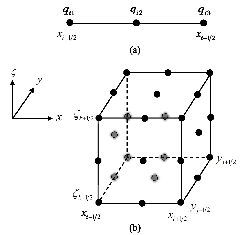Figure1. The locations (black circles) of (a) solution points in the 1D case and (b) solution points over cell C_i,j,k on a 3D Cartesian grid.


where $ {x_{i,1}} = {x_{i - {1 / 2}}},{x_{i,2}} = ({x_{i - {1 / 2}}} + {x_{i + {1 / 2}}})/2,{x_{i,3}} = {x_{i + {1 / 2}}} $.
To build the MCV scheme, two kinds of moments—namely, the VIA moment over the segment and the PV moment at the two ends—are defined as
where $\Delta {x_i} = {x_{i + {1 / 2}}} - {x_{i - {1 / 2}}}$. Then, the time evolution equations of the above moments are obtained from governing Eq. (38),
where $\hat f$ and ${\hat f_x}$ are the numerical flux function and its derivatives at cell boundary ${x_{i - {1 / 2}}}$ and ${x_{i + {1 / 2}}}$.
Given q_i,s (s = 1, 2, 3), a cell-wise Lagrangian interpolation function Q_i(x) can be built,
where
is the Lagrangian basis function.
Given interpolation function (46), Eqs. (40)?(42) can be explicitly expressed in the unknowns,
Using the relations of Eqs. (48)?(50), the evolution equations of different moments (43)?(45) are obtained as
The constraint conditions (51)?(53) finally lead to the equations to update the unknowns as follows:
At boundary points ${x_{i - {1 / 2}}}$ and ${x_{i + {1 / 2}}}$, the flux function derivatives are shared by two adjacent cells, which may lead to discontinuous values on the left and right sides. They should be computed by the approximate derivative Riemann solver. There are some existing approximate Riemann solvers available, such as the local Lax?Friedrich (LLF) solver (Shu and Osher, 1988), Roe’s solver (Roe, 1981), and the Low Mach number Approximate Riemann Solver (Chen et al., 2013). In our present model, instead of the LLF solver used in the previous 2D dynamic core (Li et al., 2013b), Roe’s approximate Riemann solver is adopted, say ${\hat f_{x,i - {1 / 2}}}$, which reads
where ${\Lambda _{i - 1/2}}$ is the matrix of eigenvalues; and ${R_{i - {1 / 2}}}$ and $R_{i - {1 / 2}}^{ - 1}$ are the matrices of the right and left eigenvectors of ${A_{i - 1/2}}$ respectively, which can be directly calculated from the point values at ${x_{i - {1 / 2}}}$. The left-side and right-side derivatives of the state variable at the cell boundary ${x_{i - {1 / 2}}}$ are computed from the Lagrangian interpolated functions by
The same procedure also applies for cell boundary ${x_{i + {1 / 2}}}$.
We write Eqs. (54)?(56) into the following vector-matrix form:
Denoting the entries of the matrix
by M_l,α (l =1, 2, 3 and α =1,…, 4), and the components of
by F_α, Eq. (60) can be written into a component form,
The 3D computational domain D is decomposed into non-overlapping mesh elements C_i,j,k indexed by i, j and k in the x, y and ζ directions respectively. Thus, we have
where the cell element spans over
with
and
and I, J and K represent the total numbers of cell elements in the x, y and ζ directions. The solution points (shown in Fig. 1b) for cell C_i,j,k are denoted by q_i,j,k,l,m,n (l, m, n = 1, 2, 3) and defined at points (x_i,j,k,l, y_i,j,k,m, ζ_i,j,k,n). For convenience, we drop the cell indices i, j and k from now on and focus on the local control volume. As addressed in Ii and Xiao (2009), multi-dimensional MCV formulation in regular Cartesian grids can be obtained by directly applying 1D formulation along each direction. The semi-discretized formulation for updating the unknowns within cell element C_i,j,k in the 3D MCV framework in Eq. (27) is then obtained as
The terms ${{M}}_{_{m,\beta }}^{(y)}$ and ${{{G}}_\beta }$ are the elements of the matrix and vector in the y direction:
A similar expression is obtained in the ζ direction:
and S(q_l,m,n) stands for the source terms.
Analogously, ${\hat g_{y,j - {1 / 2}}}$ and ${\hat g_{y,j + {1 / 2}}}$ are the derivatives of the numerical flux at cell boundaries in the y direction, while ${\hat h_{\zeta,k - {1 / 2}}}$ and ${\hat h_{\zeta,k + {1 / 2}}}$ are those in the ζ direction.
So far, we have described the spatial discretization procedure of the three-point MCV scheme, and the resulting semi-discrete system of Eq. (65) is then solved by the third-order Total Variation Diminishing Runge?Kutta method (Shu, 1988) for time integration.
We denote the right-hand side of Eq. (65) by R(q_l,m,n):
The values $q_{l,m,n}^\kappa $ at time step κ are updated by the following steps to obtain the values $q_{l,m,n}^{\kappa + 1}$ at time step κ+1:
where $\Delta t = {t^{\kappa + 1}} - {t^\kappa }$ is the interval of time integration.

In this section, some standard benchmark tests are conducted in order to validate the computational accuracy and the performance of our 3D MCV dynamic core. A rising thermal bubble in a uniform environment is utilized to check the model’s ability in simulating atmospheric thermodynamic motions. Then, flow over a lower terrain in the linear hydrostatic range is considered for validating mountain waves triggered by a gentle slope. Thirdly, a strongly stratified flow past a steep isolated hill is simulated to assess the performance of the model in handling complex topography. The dynamic viscosity and Coriolis force are not included in these idealized cases. Before detailing the test cases, it is necessary to describe the boundary conditions used in the model.

2

-->

4.1. Boundary conditions

In the following test cases, two types of boundary conditions are used, including a no-flux boundary and nonreflecting boundary.
The no-flux boundary condition aims to omit the normal component of the velocity and only keep the tangential component. For velocity vector u, we enforce
where n is the outward normal vector from the boundary. Specifically, the velocity vector on one side of the boundary is equal to its negative value on the other side, while the scalar variables are copied directly.
The commonly used method of imposing nonreflecting boundary conditions involves adding absorbing layers (damping layers) along the lateral and top boundaries, which guarantee the waves exiting the domain of interest without reflection. This damping is added to the momentum and potential temperature evolution equations and always takes the following form:
where τ is the coefficient of the absorbing layer and q_b is the prescribed reference state. The strength of the damping is determined by parameter τ, which is defined differently in different works. Here, following Giraldo and Restelli (2008), it is denoted as
where τ₀ = 2.0 × 10^?2 s^?1, ${s_{\rm{c}}} \in (x,y,\zeta)$ is a location in the computational area, s₀ indicates the position of the boundary, and s_T is the thickness of the damping layer. In the overlapped region, we use the maximum of the coefficients in three coordinate directions.

2 -->

4.2. Test cases

3 -->

4.2.1. Rising thermal bubble

This test is taken from Marras et al. (2013). The domain is bounded within [0, 3200] m × [0, 3200] m × [0, 4000] m. The mesh resolution is set to 80 m. This test case uses a hydrostatically balanced reference state based on a uniform potential temperature θ₀ = 300 K. No-flux boundary conditions are applied along all six boundaries. The initial u velocity, v velocity and w velocity are set to zero. The potential temperature perturbation has the following form:
where ${R_{\rm{c}}} = \sqrt {{{(x - {x_{\rm{c}}})}^2} + {{(y - {y_{\rm{c}}})}^2} + {{(z - {z_{\rm{c}}})}^2}} $, r = 500 m is the radius of the bubble, A = 2 K is a constant, and (x_c, y_c, z_c) = (1600, 1600, 500) m. The model is run for 480 s without orography.
The initial potential temperature perturbation field and the simulated results after 480 s are shown in Fig. 2. The thermal bubble (Fig. 2a) is located in the center of the domain in the beginning. The warm perturbation generates acceleration in the inner region of the bubble, accompanied by downdrafts on either side of the bubble. Since the highest temperature inside the bubble is located in the center, the center of the bubble rises faster. This creates sharp temperature gradients in the upper part of the bubble. After 480 s, it evolves into a classical mushroom shape. Similar to previous studies such as Chen et al. (2013) and Marras et al. (2013), the present model captures the evolution of the bubble in time, and the flow structures are reproduced with high solution quality. Figures 2b?d display the xz cross section of potential temperature perturbation, horizontal wind and vertical wind at 480 s. As expected, the evolution of potential temperature perturbations remains axisymmetric at all times and is very competitive when compared to that of Marras et al. (2013) (see their Fig. 19), which applies the variational multiscale stabilization (VMS) method to suppress the instabilities of dominated convection in the centered-nature finite element framework. Different from the VMS method, the MCV scheme combined with the approximate Roe solver presents small oscillations of potential temperature perturbations in the larger gradient of the mushroom edge. The horizontal wind and vertical wind at 480 s look closely like those of Marras et al. (2013) as well. In a quantitative manner, the front of the bubble finally reaches the height of approximately 2400 m, which agrees well with Marras et al. (2013). By comparing the thermal bubble test results with previous studies, the results of the 3D MCV nonhydrostatic model look very competitive.
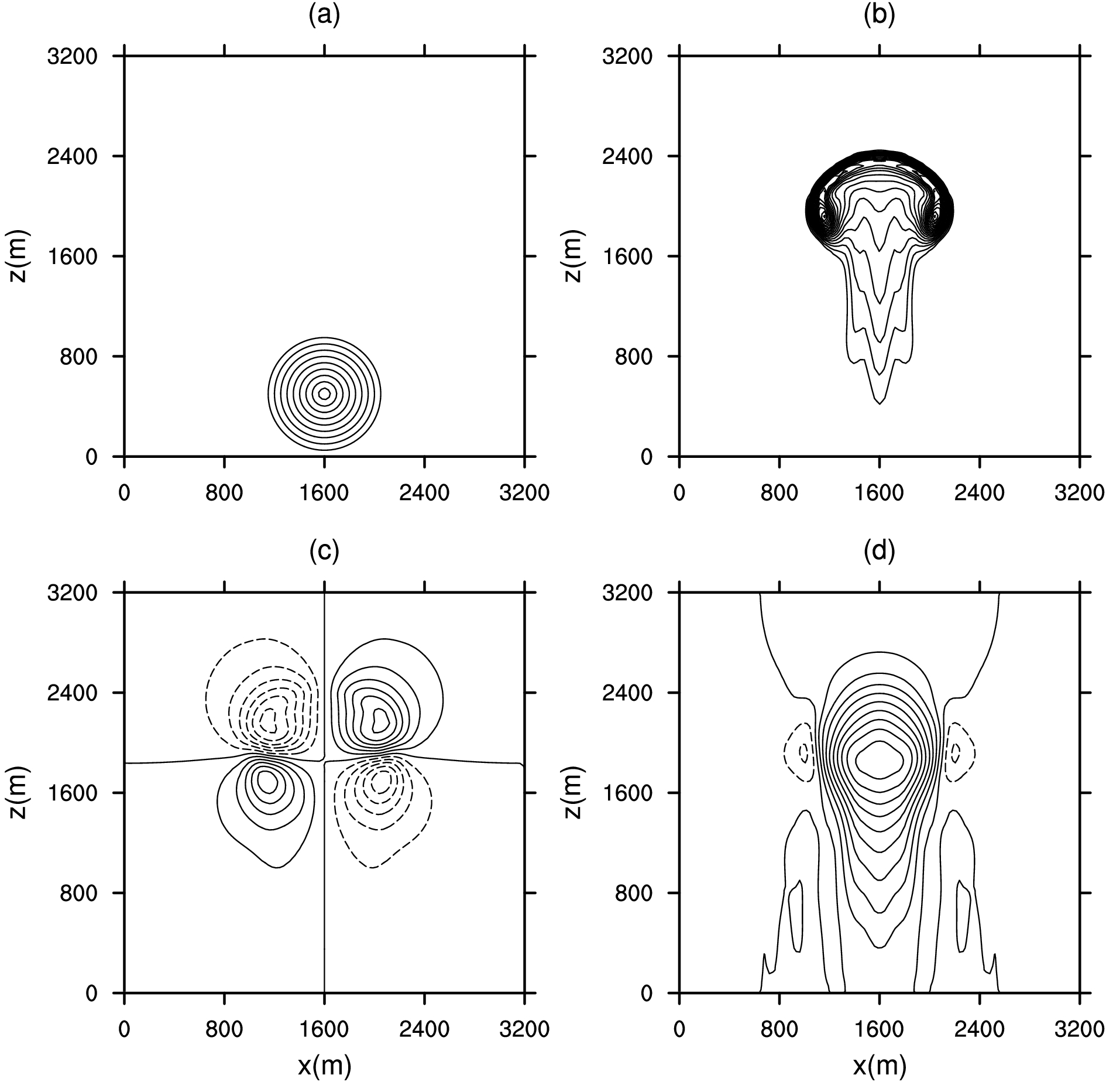Figure2. Numerical results of a 3D rising thermal bubble (xz slices at y = 1600 m). The contour lines of (a) potential temperature perturbation (units: K) at T = 0 s are from 0.0 to 2.0 with an interval of 0.2, (b) potential temperature perturbation (units: K) at T = 480 s are from 0.05 to 1.0 with an interval of 0.05, (c) the u wind (units: m s^?1) at T = 480 s are from ?2.4 to 2.4 with an interval of 0.4, (d) the vertical wind (units: m s^?1) at T = 480 s are from ?2 to 9 with an interval of 1. Positive contours are presented with solid lines and negative contours with dashed lines.



3 -->

4.2.2. 3D linear hydrostatic mountain

In this test, the initial state consists of an isothermal atmosphere with $ {\bar T} $ = 250 K, which means a constant Brunt?V?is?l? frequency $N = {g / {\sqrt {{c_p}\overline T } }}$. A constant mean flow u = 20 m s^?1 is imposed. The mountain profile is defined as
where h_c = 1 m is the mountain height, a_c = 10 km is the half-width of the mountain, and (x_c, y_c) = (120, 120) km is the center position of the mountain. The domain is [0, 240] km × [0, 240] km × [0, 24] km, with grid spacing of ?x = ?y =1500 m and ?ζ = 300 m. While no-flux boundary conditions are imposed along the bottom boundary, nonreflecting boundary conditions are used near the upper and lateral boundaries. The sponge layers are placed in the region of ζ ≥18 km for the upper boundary and the thickness of 60 km for the lateral boundaries. As mentioned in section 2.2, the hybrid vertical coordinate (Sch?r et al., 2002) is employed. It can be verified that the Froude number U/(Nh₀) > 1, so the flow is in the hydrostatic range. The model runs for five hours.
Figures 3a and b show the numerical results of the u velocity perturbation and vertical velocity after one hour, respectively. The results present the features of vertically propagating, with a small tilt component, which are in good agreement with the results reported in Giraldo (2011). The density perturbation field after five hours is plotted in Fig. 4a. Thanks to the theory of Smith (1988), the analytic solution of this problem has been made available. Our results are well matched with the analytic solution (Smith, 1988) near the mountain, but deviate away from the mountain due to the influence of the Rayleigh damping layer. We should not expect to agree exactly with the analytic solution, for it is solved under the linear Boussinesq approximation. Therefore, the results of previously published work are also used for comparison. We observe agreement with the results of Blaise et al. (2016) (see their Fig. 16a), suggesting our model is correctly capturing the mountain waves triggered by the gentle slope. It is worth mentioning that, compared with the results of Blaise et al. (2016) obtained by the discontinuous Galerkin method, our simulated density perturbation field shows small oscillations, especially at the lower levels. Additional verification is performed by comparing the density perturbations along the line x = y = 120 km. It is noted that the simulated vertical profile in Fig. 4b matches closely with the reference work (Blaise et al., 2016, Fig. 16b). In general, our 3D MCV nonhydrostatic model simulates the linear hydrostatic mountain waves quite well.
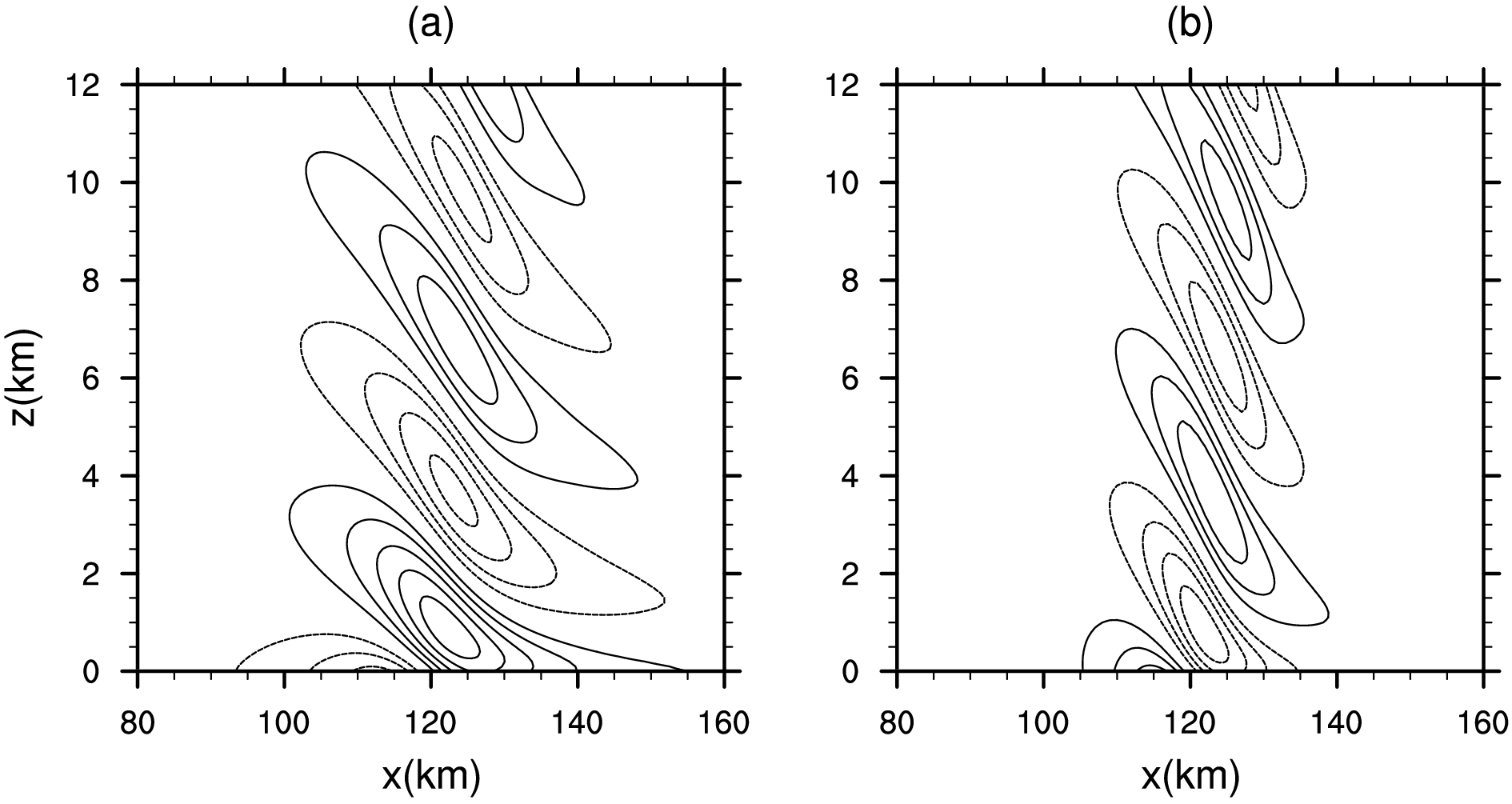Figure3. Numerical results of a 3D hydrostatic mountain after one hour (xz slices at y = 120 km). The contour lines of (a) the u velocity perturbation (units: m s^?1) are from ?0.008 to 0.01 with an interval of 0.002, and (b) the vertical velocity (m s^?1) are from ?0.002 to 0.0015 with an interval of 0.0005. Positive contours are presented with solid lines and negative contours with dashed lines. Zero contour lines are not shown.


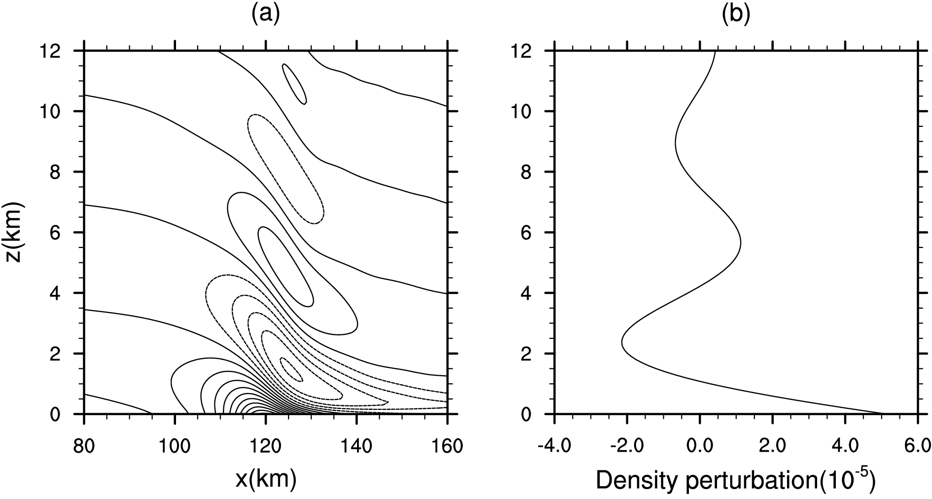Figure4. Density perturbations (units: kg m^?3) for the linear hydrostatic mountain after five hours. (a) xz cross section in the plane y = 120 km. The contour lines are from ?2.5 × 10^?5 to 5.0 × 10^?5 with an interval of 5 × 10^?6. Positive values are displayed by solid lines and negative values by dashed lines. (b) Vertical profile at x = y = 120 km.



3 -->

4.2.3. Stratified flow past a steep 3D hill

In this test case the simulations of the complex flow behind a steep isolated hill are challenging for the newly developed numerical model. The steep isolated hill is defined by
where the peak height of the hill h₀ = 1500 m, the half-width L = 3000 m, and r is the distance to the mountain center (x₀, y₀). A plot of the hill profile is shown in Fig. 5. The domain size is [0, 15 000] m × [?6000, 6000] m × [0, 6000] m, respectively, in the x, y and ζ direction. The mesh consists of 151 × 121 × 61 grid points with uniform grid spacing ?x = ?y = ?ζ = 100 m. The model is integrated up to 1200 s when the main features of the solution are already established. The sponge layer extends upward from a height of 4500 m and at the lateral outflow boundary with 1500 m thickness. Following Smolarkiewicz et al. (2013), the initial state is characterized by uniform horizontal wind (u = 5 m s^?1) with constant buoyancy frequency (N = 10^?2 s^?1). The reference potential temperature is θ₀ = 300 K. The specified environmental profile and the height of the hill result in a low Froude number flow. Here, the Froude number equals 1/3. The flow is in the nonhydrostatic range. This test case also complements the quantitative test of our 3D nonhydrostatic model. For convenience of comparison, the same contour intervals in the figures of this test case are used as in previous studies.
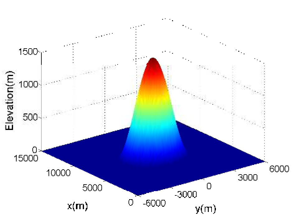Figure5. The steep 3D hill profile. Units: m, in both the horizontal and vertical direction.


Figure 6 shows the vertical velocity along the lower surface of z = h(x, y). Wind vectors are overlaid on the contours of vertical velocity. It can be seen in Fig. 6 that the symmetric structures of both vertical velocity and wind vectors are perfectly reproduced, similar to previous studies (Smolarkiewicz et al., 2013), especially the two large eddies on the lee side and the lower flow splitting.
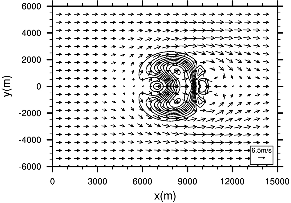Figure6. Vertical velocity (units: m s^?1) along the lower surface of z = h(x, y). The contour lines are from ?5.0 to 1.0 with an interval of 0.5. Positive values are denoted by solid lines and negative values by dashed lines. Zero contour lines are not shown. Vector arrows are overlaid.


Figure 7a displays the vertical velocity in the central xz cross section (y = 0). This figure is generated by linearly interpolating the vertical velocity in the transformed coordinate ζ to the geometric height coordinate z. It can be seen that the MCV nonhydrostatic model captures fine-scale features of the turbulent wake on the lee side and the gravity-wave response aloft. The magnitude of vertical velocity also agrees quantitatively with the simulation of Smolarkiewicz et al. (2013). In comparison with the reference results (Smolarkiewicz et al., 2013; Szmelter et al., 2015), our model introduces small spurious noises, although numerical dissipation is not imposed. Additionally, our numerical results show a better simulation of the positive vortex on the lee side. Therefore, we can again confirm the competitive performance of our model.
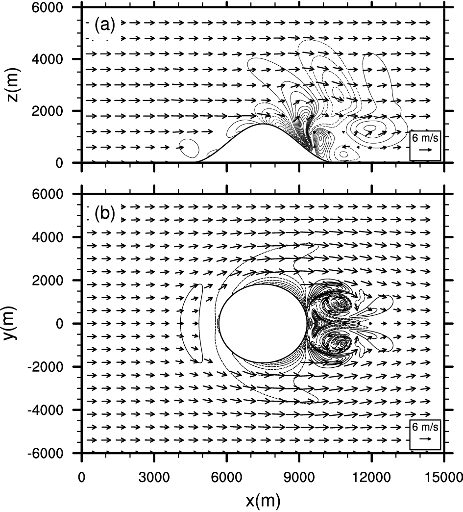Figure7. (a) Vertical velocity (units: m s^?1) in the central xz cross section at y = 0. The contour lines are from ?4.0 to 5.0 with an interval of 0.5. (b) Vertical velocity (units: m s^?1) in the xy cross section at z = 500 m. The contour lines are from ?4.0 to 3.0 with an interval of 0.5. Positive values are denoted by solid lines and negative values by dashed lines. Zero contour lines are not displayed. Vector arrows are overlaid.


The profiles of vertical velocity in the xy cross section at the height of z (= h₀/3) = 500 m are plotted in Fig. 7b. This horizontal flow patterns also compare well with existing results [see Fig. 6 in Smolarkiewicz et al. (2013) and Fig. 7 in Szmelter et al. (2015)]. The fine-scale eddy structures are perfectly resolved by our model, especially the two evident eddies behind the hill. Figure 8 gives the xy cross section of vertical velocity at z = 2500 m. No visually distinguishable differences are observed between our results and those of Smolarkiewicz et al. (2013) (see their Fig. 9). Overall, it can be seen that, without any artificial dissipation terms included in the equation set, the 3D MCV nonhydrostatic model not only simulates a smoother numerical solution, but correctly reproduces all the small-scale characteristics generated by the steep hill.
Figure8. Vertical velocity (units: m s^?1) in the xy cross section at z = 2500 m. The contour lines are from ?2.0 to 1.5 with an interval of 0.5. Positive values are denoted by solid lines and negative values by dashed lines. Zero contour lines are not displayed. Vector arrows are overlaid.

In this paper, a 3D compressible nonhydrostatic model is presented using a three-point MCV method, which extends the previous 2D MCV nonhydrostatic atmospheric dynamics to 3D in the terrain-following grid to facilitate accurate simulations in the presence of complex topography, which is a challenging task to numerical modeling of the atmosphere. In the MCV algorithm, the two kinds of moments (PV moment and VIA moment) are treated as the prognostic variables and updated through evolution equations in different forms. The constraint on the VIA moment guarantees the exact numerical conservation, while the PV moment can be computed efficiently and enables the building of high-order reconstructions in a single cell. Being a nodal-type high-order method, the MCV formulation has an apparent advantage in dealing with complex geometric terms.
The numerical results of various benchmark tests indicate that the present MCV nonhydrostatic model is very competitive when compared to most other existing advanced models. The mountain wave tests verify the capability of the present model in accurately resolving the small-scale characteristics generated by terrain effects, especially when the topographic inclination is steep. The present model is a practical and promising framework to simulate nonhydrostatic atmospheric flow.
The implementation of more complicated physical processes in the model is still in progress, and our preliminary tests with a simple wet physical process look very promising. The related results will be reported in another paper in the near future. Meanwhile, the extension of the present MCV nonhydrostatic dynamics into the spherical system is another step to be undertaken in future studies.
Acknowledgments. This work was supported by the National Key Research and Development Program of China (Grant Nos. 2017YFC1501901 and 2017YFA0603901) and the Beijing Natural Science Foundation (Grant No. JQ18001).