Kefeng ZHU^1,2,
Ming XUE^1,2,,,
Yujie PAN³,
Ming HU^4,5,
Stanley G. BENJAMIN⁴,
Stephen S. WEYGANDT⁴,
Haidao LIN^4,5

Corresponding author: Ming XUE,mxue@ou.edu;

1.Key Laboratory of Mesoscale Severe Weather/Ministry of Education and School of Atmospheric Sciences, Nanjing University, Nanjing 210023, China
2.Center for Analysis and Prediction of Storms, University of Oklahoma, Norman Oklahoma 73072, USA
3.Nanjing University of Information Science and Technology, Nanjing 210094, China
4.NOAA Earth System Research Laboratory, Boulder, CO 80305, USA
5.Cooperative Institute for Research in Environmental Sciences, University of Colorado Boulder, CO 80309, USA
Manuscript received: 2019-01-13
Manuscript revised: 2019-07-06
Manuscript accepted: 2019-07-24
Abstract:A regional ensemble Kalman filter (EnKF) data assimilation (DA) and forecast system was recently established based on the Gridpoint Statistical Interpolation (GSI) analysis system. The EnKF DA system was tested with continuous three-hourly updated cycles followed by 18-h deterministic forecasts from every three-hourly ensemble mean analysis. Initial tests showed negative to neutral impacts of assimilating satellite radiance data due to the improper bias correction procedure. In this study, two bias correction schemes within the established EnKF DA system are investigated and the impact of assimilating additional polar-orbiting satellite radiance is also investigated. Two group experiments are conducted. The purpose of the first group is to evaluate the bias correction procedure. Two online bias correction methods based on GSI 3DVar and EnKF algorithms are used to assimilate AMSU-A radiance data. Results show that both variational and EnKF-based bias correction procedures effectively reduce the observation and background radiance differences, achieving positive impacts on forecasts. With proper bias correction, we assimilate full radiance observations including AMSU-A, AMSU-B, AIRS, HIRS3/4, and MHS in the second group. The relative percentage improvements (RPIs) for all forecast variables compared to those without radiance data assimilation are mostly positive, with the RPI of upper-air relative humidity being the largest. Additionally, precipitation forecasts on a downscaled 13-km grid from 40-km EnKF analyses are also improved by radiance assimilation for almost all forecast hours.
Keywords: satellite radiance assimilation,
EnKF,
bias correction
摘要:在之前的研究中，我们已经建立了基于区域GSI的集合卡尔曼滤波(GSI-EnKF)快速同化分析与预报系统。该系统每3小时循环更新分析，同时，基于集合平均分析场向前预报18小时，但之前的研究并没有同化卫星资料。本研究进一步同化了卫星辐射亮温观测，比较了卫星资料同化关键技术中的两种常用偏差订正方案，并分析了辐射亮温资料同化对预报的贡献。设计了两组实验，第一组实验比较了两种偏差订正方案，即采用基于GSI3DVar的变分偏差订正算法和基于EnKF算法的偏差订正算法，这组实验采用观测数据比较稳定的AMSU-A作为测试数据。结果表明：两种偏差订正算法均能有效地减小观测值和模拟的辐射亮温差异，AMSU-A同化减少了多数预报量的预报误差。第二组实验我们测试了辐射亮温观测同化对预报的影响，同化数据包括AMSU-A、AMSU-B、AIRS、HIRS3/4和MHS，与没有卫星资料同化实验相比，多数预报变量的误差减少百分比（RPI）大于零，表明卫星资料同化减少了多数预报变量的预报误差，其中相对湿度改进最为明显。基于40 km的GSI-EnKF快速分析，嵌套了13 kmWRF预报，结果也表明，基于卫星资料同化的分析场的降水预报评分技巧要高于没有卫星资料同化的分析场。
关键词:GSI-EnKF快速更新分析与预报循环系统,
卫星资料同化,
偏差订正

HTML

--> --> -->

The quality of short-range weather forecasts depends, to a large extent, on the accuracy of model initial conditions (Sun et al., 2014). Compared to radiosonde and other conventional observations, satellite observations usually have wider coverage and are the most important data over the oceans (Le Marshall et al., 2007). In fact, satellite data assimilation (DA) is responsible for much of the forecasting skill improvement in global NWP models over recent decades, especially in the Southern Hemisphere (Le Marshall et al., 2007).
However, studies on the impact of satellite radiance data within regional models, especially those that focus on continental regions, are relatively few. Zapotocny et al. (2005a, b) studied the relative impacts of Geostationary Operational Environmental Satellite (GOES) and Polar Orbiting Operational Environmental Satellite (POES) radiance data versus rawinsonde data within the National Centers for Environmental Prediction (NCEP) Eta (Black, 1994) three-dimensional variational (3DVar) DA system (Rogers et al., 1996). They found that GOES data had a larger impact on 24-h forecasts than the POES data for most of the levels and seasons examined, while the only components of POES data showing appreciable forecast impacts were the combined Advanced Microwave Sounding Unit A and B (AMSU-A and -B) data and the Special Sensor Microwave/Imager Precipitable Water (SSM/I PW) data. The individual components of the POES Microwave Sounding Unit, High Resolution Infrared Radiation Sounder (HIRS) and SSM/I wind data exhibited little impact at 24 h (Zapotocny et al., 2005b). Other studies have focused on a specific sensor (McCarty et al., 2009) or a case (Liu et al., 2012; Schwartz et al., 2012). Collectively, their results showed that both the analyses and forecasts were improved by assimilating radiance.
Encouraging as they are, the assimilation of satellite radiance observations in regional models has not led to consistently better results as in global models. Most recently, Kazumori (2014) examined the impact of radiance data from various satellite systems in the Japan Meteorological Agency operational mesoscale four-dimensional variational system. When verified against sounding data, their forecasts showed slightly negative impacts above 500 hPa and positive impacts below. Similar results are also reported in Lin et al. (2017b), who found small consistently positive impacts between 800 and 400 hPa for AIRS DA within the operational Rapid Refresh (RAP) system (Benjamin et al., 2016), but not always positive impacts at levels above and below.
To effectively assimilate radiance data, bias correction is essential and the key to successful radiance assimilation. Rizzi and Matricardi (1998) summarized the possible discrepancies between measured and simulated radiances. Firstly, errors from preprocessing of observations. For example, most of the radiance data used in operational models are clear-sky radiance. But until now, most cloud detection algorithms are threshold-based, in which thresholds are often set empirically (Zou and Da, 2014). Accurate detection for all types of clouds is still challenging. Secondly, errors from the forward observation operator model. The simulated radiance over land is less accurate than over ocean due to the complexity of the surface emissivity of land (Karbou et al., 2010). Also, the simulated radiance is less accurate in cloud-contaminated regions than in clear-sky conditions (Bauer et al., 2010). Finally, errors from the model background. Biases in the forecast background are common issues for NWP models. For a specific system, forecast biases due to the use of specific empirical physics schemes is inevitable (Fan and van den Dool, 2011).
Bias correction for limited-area frequently updated forecast systems has unique challenges compared to that for global forecast systems. The accuracy of bias correction largely depends on the size of usable data samples. The number of available radiance observations in regional models depends strongly on the satellite location, while in global models the total number is almost constant (Kazumori, 2014). Besides, shorter data cutoff time, limited extent of the model domain, and lower model top in regional models all reduces the available number of radiance data (Lin et al., 2017a).
Various bias correction methods have been developed in the past, including offline and online types. The former uses long-term forecasts and radiance observations to generate fixed bias correction coefficients (Harris and Kelly, 2001), while the latter incorporates bias correction into the variational (Derber and Wu, 1998; Auligné et al., 2007; Dee and Uppala, 2009) or ensemble (Miyoshi et al., 2010) DA processes. With online correction, the correction coefficients are updated within the assimilation procedure, cycle through cycle. Details of online bias correction methods will be introduced in section 2.
Recently, we successfully demonstrated the advantage of the GSI-based ensemble Kalman filter (EnKF) (Zhu et al. 2013, Z13 hereafter) and hybrid ensemble-3D variational (En3DVar) (Pan et al., 2014) methods over the GSI 3DVar method for assimilating conventional observations used by the operational RAP (Benjamin et al., 2016) system. Those studies, however, did not include satellite data, because initial tests did not show clear positive impacts. As discussed later, proper bias correction is found to be key step towards achieving positive impacts of satellite radiance data within our regional EnKF system. In this paper, two online bias correction methods are first tested within the established EnKF when assimilating AMSU-A radiance data. Then, all radiance data available are assimilated and their impacts on the subsequent forecasts are evaluated.
The rest of this paper is organized as follows. In section 2, a brief introduction to the current GSI-based EnKF system is presented together with a description of the radiance data and bias correction procedures. Experimental design and verification metrics used are described in section 3. The behaviors of the two bias correction methods on short-range forecasts are first investigated in section 4 using AMSU-A data within the EnKF framework. In section 5, the impacts of assimilating the full suite of satellite radiance data using the EnKF are further examined. A summary and further discussion are given in section 6.

2

-->

2.1. Brief review of the GSI-based EnKF system

In Z13, an experimental GSI-based EnKF DA system was established and tested at 40-km grid spacing with 40 ensemble members and three-hourly assimilation cycles. The system was intended to be a prototypical system for the operational RAP (Benjamin et al., 2016), and the forecast model was configured based on the operational RAP except for the assimilation interval and resolution. The operational RAP runs hourly and has an approximate 13-km grid spacing. The choice for the current EnKF tests was dictated by the availability of computational resources required by a large number of sensitivity experiments with continuous cycles. Another consideration is the potential use of a lower-resolution EnKF in combination with a higher (native) resolution EnVar in a dual-resolution EnKF-EnVar hybrid setup (Schwartz et al., 2015; Pan et al., 2018) to save computational cost of operational implementation.
The eventual goal is to provide hourly ensemble perturbations to the operational RAP hybrid DA system. As a pilot study, an EnKF-En3DVar hybrid DA system at 40-km grid spacing was established based on the RAP system in Pan et al. (2014), and more recently a dual-resolution version that uses ensemble covariance downscaled from the 40-km EnKF DA system has also been tested (Pan et al., 2018). Results show consistent advantages of EnKF and hybrid En3DVar over GSI 3DVar, and that the hybrid DA further improves upon EnKF in some aspects of forecasts. These earlier encouraging results prompted the implementation of hybrid En3DVar DA for the operational RAP, but it borrows ensemble perturbations from the NCEP GFS EnKF system instead of producing them using RAP’s own EnKF (Hu et al., 2017; Wu et al., 2017), partly due to computational constraints. The current operational 13-km RAP hybrid DA uses 25% and 75% static and ensemble background error covariances, respectively (Benjamin et al., 2016), with the GFS EnKF perturbations available only every six hours and with delayed availability. For optimal results, it is desirable to operationally implement RAP’s own EnKF DA cycles, and to couple these with the EnVar hybrid DA system. Our prior and current studies represent some of the efforts toward such a goal.
For the cycled ensemble DA system, the lateral boundary conditions are from three-hourly NCEP GFS forecasts but perturbed using the “randomCV” option of the WRF DA system (Barker et al., 2012) following Torn et al. (2006). The same method was used to generate perturbations for initializing the first EnKF DA cycle. For the GSI-based EnKF system, the observation innovations, y ? H(x), are calculated within GSI and then used within the EnKF system. The analysis algorithm is the ensemble square root filter of Whitaker and Hamill (2002). Forty-member ensemble forecasts are run for three hours between the analysis times, while 18-h short-range deterministic forecasts are run from the ensemble mean analyses of each cycle. As in Z13, a modified digital filter launch procedure (Lynch and Huang, 1994) where the land surface fields are subject to the same filtering, is used before launching the forecasts. All members use the same physics options, including Grell-G3 cumulus parameterization, Thompson microphysics, RRTM longwave radiation, Goddard shortwave radiation, the MYJ planetary boundary layer scheme, and the RUC-Smirnova land-surface model. In short, the EnKF DA system used is the same as that described in Z13, and the specific configurations are the same as experiment EnKF_CtrHDL of Z13, except for the addition of satellite radiance data and global positioning system (GPS) PW (Smith et al., 2007).
Following Z13, height-dependent background error covariance localization scales are used, in which the horizontal covariance localization scale increases from 700 km at the surface to 1050 km at the model top. The vertical localization scale ln(p_cut) depends on the analysis variable. For relative humidity (RH) and temperature, it is set to a quarter and one half of 1.1 at the surface and model top, respectively. For horizontal wind components, U and V, the vertical correlation length is twice as large as that for RH and temperature. A value of 1.6 is used for surface pressure observations. These settings were found to produce the best results in Z13 based on sensitivity experiments. Here, the vertical localization scale for radiance observations is 1.6. The covariance inflation used is the same as in Z13, containing a fixed and an adaptive part (Anderson, 2009; Whitaker and Hamill, 2010). For the experiments with satellite radiance assimilation, the coefficient of the fixed part, b in Eq. (5) of Z13, is increased from 0.1 (no satellite radiance assimilation) to 0.16 (AMSU-A radiance assimilation) and 0.18 (full radiance assimilation). This is because the ensemble spread tends to be reduced when more satellite observations are assimilated. More details on other settings can be found in Z13.
For radiance assimilation, GSI uses the Community Radiative Transfer Model (CRTM) developed by the Joint Center for Satellite Data Assimilation (Han et al., 2006; Weng, 2007) as its observation operator. CRTM is capable of simulating most geostationary/polar-orbiting satellite observations, covering microwave and infrared frequencies.

2 -->

2.2. Assimilation data

The radiance data assimilated in this study include AMSU-A, AMSU-B, AIRS, as well as the Microwave Humidity Sounder (MHS) and High-resolution Infrared Radiation Sounder (HIRS/3 and HIRS/4) instruments on polar-obitting satellites. These data were part of the operational RAP and GFS observation data streams. For a regional, frequently updated forecasting system, radiance data preprocessing is an important step towards obtaining a positive impact of radiance assimilation (Lin et al., 2017a). To be consistent with the three-hourly assimilation cycles tested in this paper, the radiance data are reprocessed into three-hourly data batches, including data within the ±1.5-h windows centered on the analysis times. In this study, clear-sky radiance data are assimilated. GSI uses the minimum residual method to detect clouds (Eyre and Menzel, 1989). Additionally, for the quality control step, GSI uses outliers to reject observations along the scan edges. Table 1 gives the GSI default values for each sensor. Note that some satellite sensors have higher spatial resolution, and hence more scan points than others. In general, about 10% of the scan points along both left and right edges were removed.

Sensor name	Number of scan points	Left bound	Right bound
AMSU-A	30	4	27
AMSU-B	90	10	81
MHS	90	10	81
HIRS	56	7	50
AIRS	90	10	81

Table1. Lists of scan points used by GSI for each satellite sensor. Points outside the left and right bounds are removed.


Figure 1 shows the number of assimilated data for each channel used and the corresponding height level of the maximum response function. AMSU-A and MHS are at microwave frequency, while AIRS and HIRS are at infrared frequency. For infrared sensors, the number of assimilated data is smaller near the surface compared to higher-level channels (Figs. 1a, e and f). This is especially true for infrared sensors such as HIRS4 (Figs. 1e and f). AIRS behaves similarly but benefits from more channels available near the surface (Fig. 1b), and the total number of near-surface data is still large (Fig. 1a). In fact, for this study, the total number of assimilated AIRS data is the largest. For microwave sensors, the number of surface channel data is not as many as for upper-level channels, but is still comparable (Figs. 1c and g). AMSU-A mainly provides atmospheric temperature profiling with data from several satellites and provides by far the best coverage. Among all instruments, the amount of assimilated AMSU-A data is the second largest. In all, the satellite radiance data from multiple sensors and satellites provide a reasonably good coverage in the 3D model domain over a period of time.
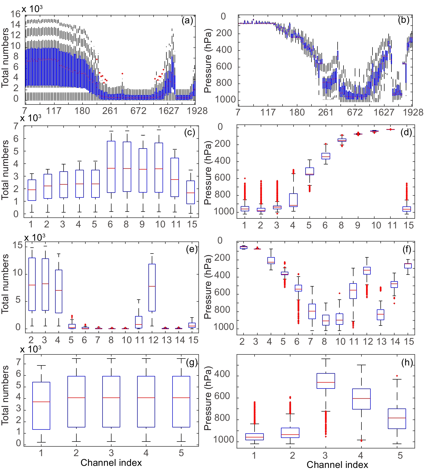Figure1. Number of assimilated observations (left) and corresponding heights (of the level of maximum response function, right). The first to fourth rows are for AIRS, Metop AMSU-A, HIRS4, and MHS, respectively. Here, only used channels are displayed. The x-axis is the channel index.



2 -->

2.3. Introduction to two online bias correction schemes

Online bias correction methods can be classified into variational versus non-variational approaches. Variational bias correction estimates the correction coefficients simultaneously with state estimation within a variational framework. Specifically, in a 3DVar framework, the cost function, following Dee and Uppala (2009), is given by
where
is the correction to the departure of simulated radiance ${H_2}({{x}})$ from radiance observations ${{{y}}_2}$. Here, the modified 3DVar cost function $J$ includes the estimation of bias correction coefficients in coefficient vector $\,{\beta }$, which are analyzed together with state vector x. We write the observation term in two parts: one for radiance data ${{{y}}_2}$, and one for all other observations ${{{y}}_1}$, which are associated with the corresponding error covariances R₁ and R₂, and observation operators H₁ and H₂. ${{{x}}_{\rm{b}}}$ is the background state vector, and x is the state vector to be analyzed. ${{\beta }_{\rm{b}}}$ is the prior estimate of bias correction coefficient. ${{{B}}_x}$ and ${{{B}}_\beta }$ are the error covariance matrices for the background state and bias parameters, respectively. The radiance data are corrected using the bias correction vector ${{b}}$ given by Eq. (2), which depends on predictors in P. Those predictors are usually air-mass dependent (Flobert et al., 1991). Subscript i represents the index of predictors, N_p is the number of predictors. p_i represents individual column vector i of matrix P. In the version of GSI used in this study, there are five predictors for bias correction, including the global offset, zenith angle predictor, cloud liquid water (CLW) predictor, temperature lapse rate (TLR) predictor, and the square of the TLR predictor. In the version used, the scan-angle component is still updated outside GSI (Derber and Wu, 1998) using the moving average of the weighted differences between the quality controlled radiance observations and the first guess. More recent versions of GSI have incorporated this term into the variational estimation (Zhu et al., 2014).
Equations (3) and (4) give an example of how the predictor terms CLW and TLR are calculated within GSI for the Metop AMSU-A sensor:
Here, ${\rm{B}}{{\rm{T}}_{{\rm{sim}}}}$ and ${\rm{B}}{{\rm{T}}_{{\rm{obs}}}}$ are the simulated and observed brightness temperature, respectively. The numbers indicate channels 1 and 2; d₁ = 0.754 and d₂ = ?2.265 are weight coefficients. Based on Eqs. (3) and (4), CLW is not channel-dependent, while TLR is. In Eq. (4), $\tau $ is the transmittance and T is the model background temperature. Index k represents the vertical level, while N is the number of vertical levels. T₀ is surface temperature. Figure 2 shows an example of TLR calculated using the US standard atmosphere profile for the Metop AMSU-A sensor. The changes of transmittance between levels $\Delta \tau = \tau (k) - $$ \tau (k + 1)$ are very similar to vertical weighting functions (not shown). $\Delta \tau $ is always positive (Fig. 2a). For TLR, channels 1?6 are positive. Among these, channels 4 and 5 have clearly larger TLR values than other channels. As the temperature gradient $\Delta T = T(k - 1) - T(k + 1)$ turns to be negative at some high levels, the TLR of channels 8?11 become negative. Channel 15 is an exception since it also peaks near the surface.
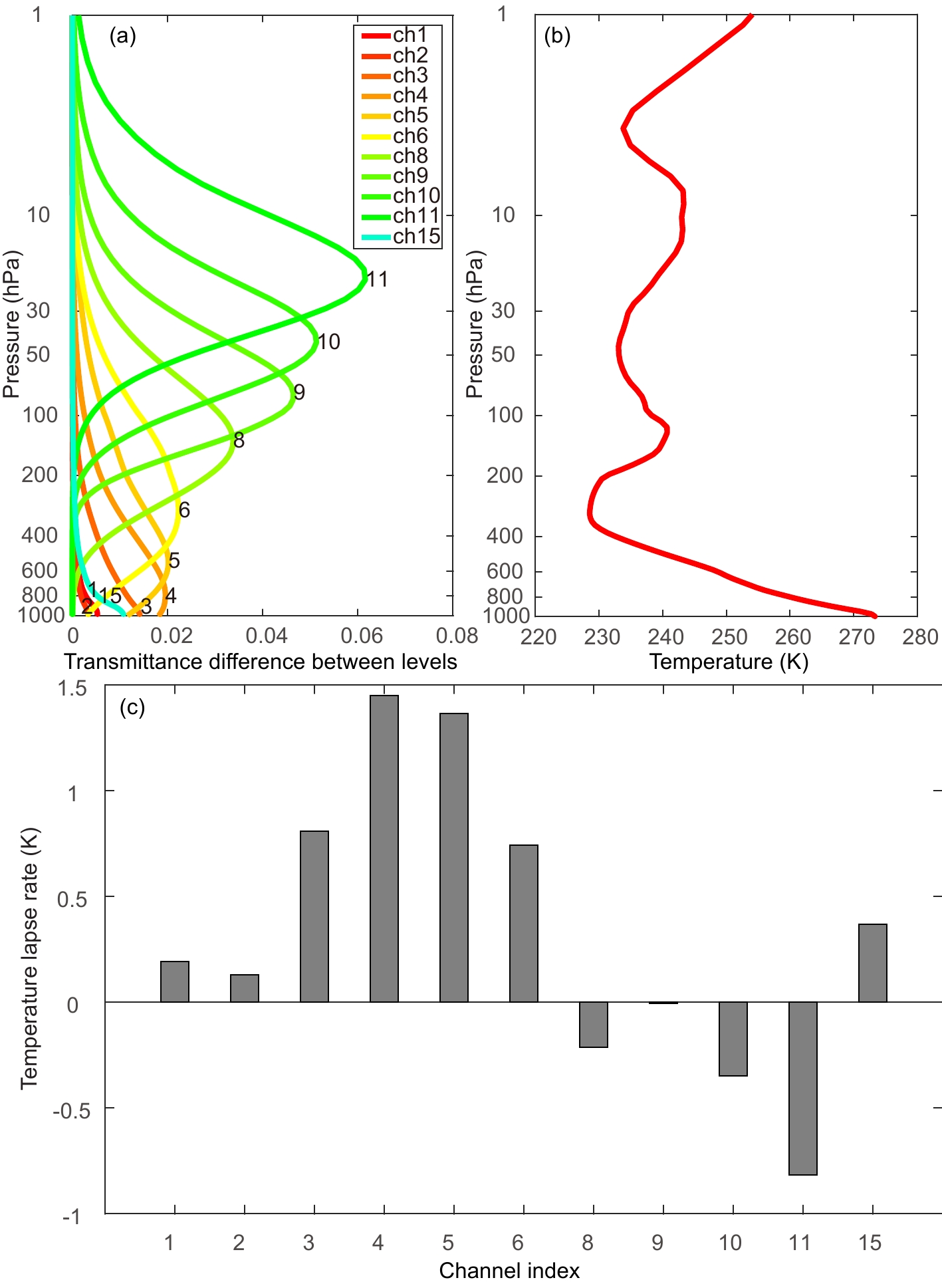Figure2. (a) Vertical profiles of transmittance changes for Metop AMSU-A, (b) vertical profile of temperature, and (c) bias corrected term of the temperature lapse rate. All figures are plotted using US standard atmosphere within the CRTM. Only channels that are finally assimilated are given.


The other non-variational bias-correction approach uses the EnKF analysis equation to update the bias-correction coefficients or predictors, and it is performed within each cycle before state estimation (Miyoshi et al., 2010). Setting the derivative of cost function J in Eq. (1) with respect to $\,{\beta }$ to zero yields the following optimal update equation for the increment of bias correction coefficient vector, $\delta {\beta }$:
where only satellite data in vector ${{y}_2}$ are used. The above formulation can be shown to be mathematically equivalent to the 3DVar solution for a linear and Gaussian system, which also has the same form as the EnKF analysis update equation (with the inclusion of online bias correction) (Kalnay, 2002). Here, B_β is assumed to be diagonal and the diagonal elements are assumed to be 0.1, which is also the GSI default value. Within the EnKF system, we apply bias correction to observation priors using prior estimated bias correction coefficients. Equation (5) is used to update $\,{\beta }$ after state estimation. After $\delta {\beta }$ is obtained, the bias correction coefficients $\,{\beta }$ are updated according to
We note here that the coefficient estimation in Eq. (5) appears independent of the state vector estimation, while the estimation of the coefficients using the cost function in Eq. (1) involves state vector x. This is because the EnKF algorithm is sequential; the correction coefficients are updated using the updated state vector. In comparison, in Eq. (1), state vector x and the coefficient vector are updated simutaneously. However, because ${{B}_x}$ and ${{B}_\beta }$ are uncorrelated, the state and coefficient estimations, even in the variational framework, are not strongly linked. Still, the algorithm differences can lead to differences in results in practice, and it is a goal of this paper to compare their relative performance.
In our EnKF experiments, we use either the variational procedure that minimizes the cost function Eq. (1) or the EnKF procedure that updates the correction coefficients using Eq. (5). In Table 1, we label the former procedure “variational” and the latter procedure “EnKF ”. When the variational procedure is used to estimate bias correction coefficients for EnKF experiments (for comparison purposes), GSI 3DVar is run with full observations using the EnKF ensemble mean forecast as its background in each analysis cycle; in other words, the GSI 3DVar cycles piggyback on the EnKF cycles; the GSI 3DVar solver is therefore used purely for the purpose of variationally estimating the bias correction parameters, while its state estimation is discarded. For GSI 3DVar, two outer loops and a maximum of 50 inner iterations are imposed.
As pointed out earlier, in theory, the variational and EnKF parameter updates should be mathematically equivalent, for linear systems with Gaussian errors at least. The key difference lies in that, within a variational framework, the parameter and state estimations are performed simultaneously, while within EnKF they are updated sequentially. In addition, the variational minimization involves linearization of the observation operators.

2

-->

3.1. Experimental design

To compare with the results without satellite radiance assimilation, we continue to use the same test period as Z13, starting at 0000 UTC 8 May 2010 and ending at 2100 UTC 16 May 2010, over a total of nine days. This period features a variety of active convective weather, including the 10 May Oklahoma tornado outbreak featuring strong mesoscale forcing, a mesoscale convective system (MCS) on the night of the 11th, a cold-season type Front Range upslope low-pressure precipitation event, and some southeast propagating MCSs across Texas. The DA experiments are run in continuous three-hourly updated cycles. The assimilation domain has a horizontal grid spacing of 40 km, with 207 × 207 × 50 grid points, and covers the whole of North America (Fig. 3). The model top is at 10 hPa. As described in Z13, the use of a relatively short nine-day period was mainly due to computational resource constraints; however, this length appears long enough for the EnKF state estimation and bias correction to stabilize [as discussed in Pan et al. (2014)].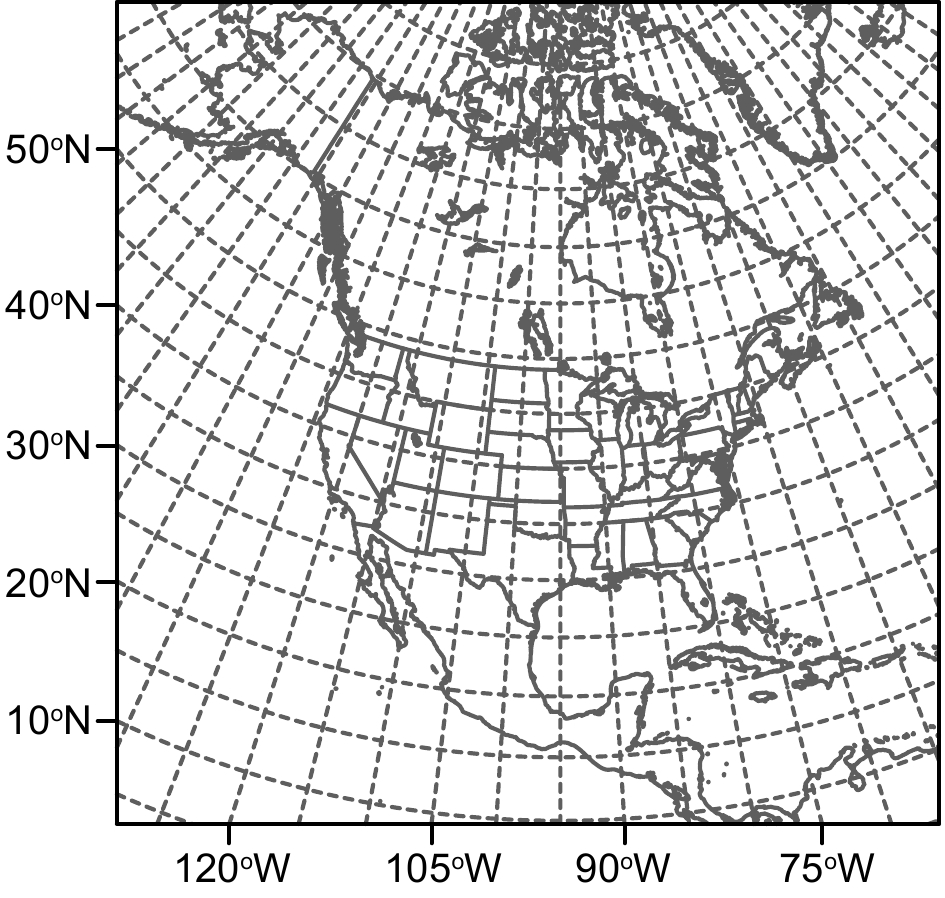
Figure3. Horizontal domain of the 40-km WRF forecast.


Table 2 lists all experiments presented in this paper. We first investigate initial bias correction coefficient issues and test the two bias correction methods in the EnKF system described in section 2c. AMSU-A radiance data are assimilated since they are available from different satellites and the number of data available within the domain is much more stable than other types of radiance data. Experiments EnKF_AMSUA_VarB0, EnKF_AMSUA_VarB, and EnKF_AMSUA_VarB2 use the variational bias correction with GSI 3DVar. For the variational bias correction, ${y}$ also contains conventional observations during the update of bias correction coefficients $\,{\beta }$. In experiment EnKF_AMSUA_VarB_SP, we use only radiance observation to update $\,{\beta }$. Experiments EnKF_AMSUA_EnB use EnKF parameter estimation. Here, the number “0” in the name indicates the use of zero $\,{{\beta }_{\rm{b}}}$ in the first analysis cycle; otherwise, the recycled initial estimate of $\,{{\beta }_{\rm{b}}}$ is used. In the recycled case, the entire nine days of DA cycles are repeated, starting from the $\,{{\beta }_{\rm{b}}}$ estimated at the end of the previous pass of the nine-day cycled DA. The numbers “1” and “2” represent the recycled initial estimate of $\,{{\beta }_{\rm{b}}}$ from the zero and first run, respectively. For simplicity, the number 1 is ignored. This recycled procedure is an attempt to improve the initial guess of $\,{{\beta }_{\rm{b}}}$ when the total length of DA cycles is relatively short. Experiments with “0” are considered as spin-up runs for the correction parameter estimation and are included here mainly to see if a better initial estimate of $\,{{\beta }_{\rm{b}}}$, which is typically available in long-running DA cycles, can improve the results, given the relatively short nine-day DA period we are using. Note that in continuously cycled operational DA systems, this procedure is not necessary, and is used here to help alleviate the potential problem of the short DA period.

Experiment	Satellite radiance	Bias correction method
EnKF_AMSUA_VarB0	AMSU-A	Variational procedure, ${{\beta }_{\rm{b}}}$= 0
EnKF_AMSUA_VarB	AMSU-A	Variational procedure, using recycled ${{\beta }_{\rm{b}}}$ from EnKF_AMSUA_VarB0
EnKF_AMSUA_VarB2	AMSU-A	Variational procedure, using recycled ${{\beta }_{\rm{b}}}$ from EnKF_AMSUA_VarB
EnKF_AMSUA_VarB_SP	AMSU-A	Similar to EnKF_AMSUA_VarB, but ${{\beta }_{\rm{b}}}$ is obtained using only radiance observations
EnKF_AMSUA_EnB	AMSU-A	Similar to EnKF_AMSUA_VarB, but using EnKF procedure
EnKF_NoSat	?	?
EnKF_ALL	AMSU, AIRS, MHS, HIRS 3/4	Similar to EnKF_AMSUA_VarB, but using full radiance

Table2. List of data assimilation experiments. Here, ${{\beta }_{\rm{b}}}$ is the first guess of the bias correction coefficients vector used in the first analysis cycle. “VarB” in the experiment names stands for variational bias correction, while “EnB” stands for EnKF-based bias correction.


We then test the impact of the full set of radiance data in the EnKF system. EnKF_ALL assimilates all of the AMSU-A, AMSU-B, AIRS, MHS, HIRS3 and HIRS4 data, and is compared with EnKF_NoSat without satellite data (but with PW data included). The nine-day DA cycles are run twice, with the second time starting from the recycled estimate of $\,{{\beta }_{\rm{b}}}$ from the first pass, as in the “1” experiments. To see if the DA results produced on the 40-km grid can improve forecasts at the 13-km RAP operational resolution, 13-km forecasts from interpolated analyses of the above two experiments are run twice a day starting at 0000 and 1200 UTC, and the precipitation forecasts are evaluated.

2 -->

3.2. Verification scores

The 40-km forecasts are verified against sounding and surface observations. As in Z13, root-mean-square error (RMSE) and relative percentage improvement (RPI) are used as the verification metrics. The RPI is defined as
where the subscripts “sat” and “nosat” represent the experiments with and without satellite radiance assimilation. Positive RPI values mean reduced error or improved analyses/forecasts due to radiance assimilation.
Following Pan et al (2014), the statistical significance of RMSE differences and RPIs is determined by using bootstrap resampling (Candille et al., 2007; Buehner and Mahidjiba, 2010; Schwartz and Liu, 2014). The same method with 3000 randomly selected samples are used. For those samples, their mean and a two-tailed 90% confidence interval from 5% to 95% is calculated. For RPIs, if the bounds of a 90% confidence interval between the forecast pair are all higher than zero, it means that the improvement from the satellite assimilation experiment over the corresponding no satellite experiment is statistically significant at the 90% confidence level. In contrast, if the bounds of the 90% confidence level includes zero, it indicates a statistically insignificant difference (Xue et al., 2013; Pan et al., 2014).
For the 13-km forecasts, we focus on precipitation verification using the NCEP stage IV precipitation data as observation. Two verification scores—the Gilbert skill score (GSS) (Gandin and Murphy, 1992) (also known as the equitable threat score) and frequency bias (FBIAS)—are calculated over the contiguous US.

Bias correction accuracy largely depends on the estimated bias correction coefficients. Liu et al. (2012) ran prior three-month offline statistics to get an initial $\,{{\beta }_{\rm{b}}}$. In Schwartz et al. (2012), the spinup time period of bias correction coefficients is about a week. In their paper, a 6-h assimilation cycle interval is used. In this study, the assimilation cycle interval is three hours. This greatly reduces the number of samples at a given analysis time, which may have large impact on the stabilization of bias correction coefficients.
To examine the required duration for the coefficients to stabilize, Fig. 4 presents the time series of bias correction coefficients through the assimilation cycles. Here, we take the values of $\,{{\beta }_{\rm{b}}}$ of NOAA-15 AMSU-A channel 5 as an example using variational bias correction methods. Choosing other channels or using the EnKF-based bias correction method result in similar behaviors and are not shown. To see if more cycles are helpful, in the EnKF_AMSUA_VarB2 experiment, we repeat the nine-day DA cycles starting from the coefficients from the last cycle of EnKF_AMSUA_VarB. In EnKF_AMSUA_VarB0, the coefficients of different predictors become stable after a few days of spin up. The coefficients of the CLW predictor and the TLR predictor equilibrate in less than two days (Figs. 4b and c). Coefficients of the zenith angle predictor and the square of the TLR predictor take longer to stabilize but also approach nearly steady states after seven days or so (Figs. 4a and d). Starting from the recycled $\,{{\beta }_{\rm{b}}}$, the coefficients require virtually no spin up in EnKF_AMSUA_VarB and are more or less stable throughout the nine-day cycles. Even more cycles in another pass of the nine-day DA in EnKF_AMSUA_VarB2 produce little systematic change in the correction coefficients, suggesting that the nine days of the testing period is long enough to produce reliable results as far as the bias correction procedure and the data impacts are concerned, especially when a better initial guess of the coefficients obtained from a trial experiment is used. In the following, all experiments are conducted twice, with the first discarded as a spin-up run, for the purpose of getting a better initial guess of $\,{{\beta }_{\rm{b}}}$.
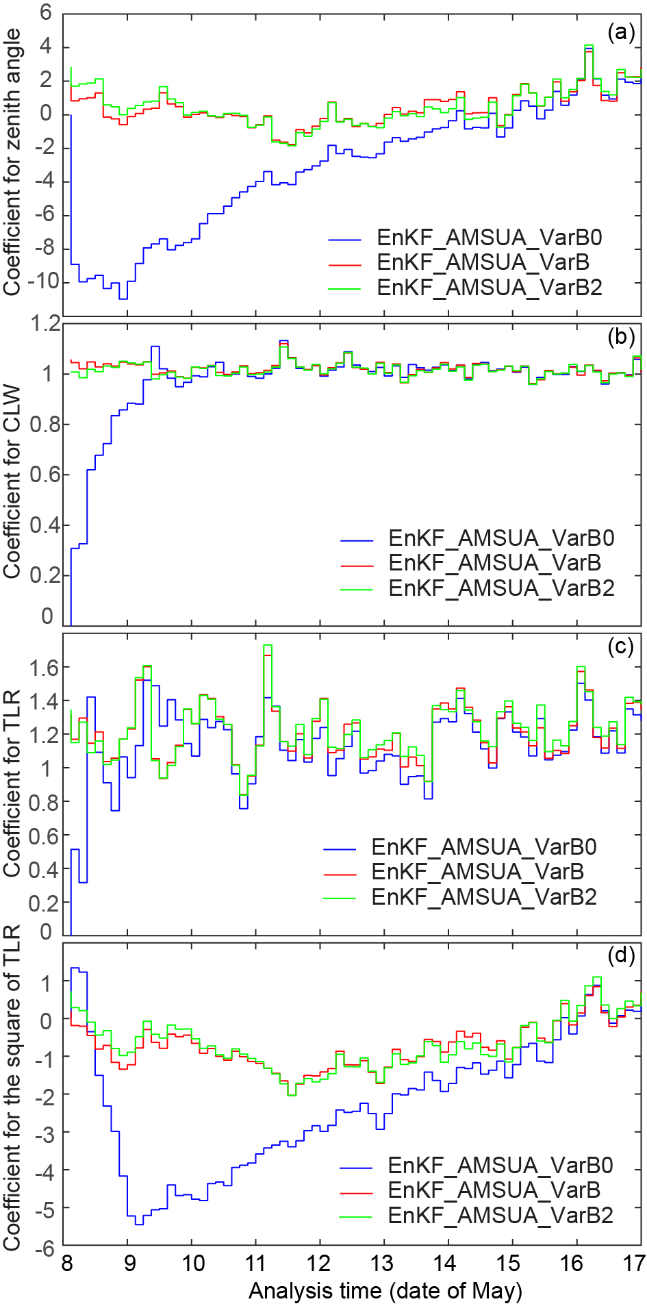Figure4. Bias correction coefficients through the assimilation cycles. Here, NOAA-15 AMSU-A channel 5 is used as an example. Panels (a?d) are for the coefficients for the zenith angle predictor, cloud liquid water predictor, temperature lapse rate predictor, and the square of the temperature lapse rate predictor, respectively. The x-axis marks the date of the test period. For example, “8” represents 0000 UTC 8 May 2010.


Figure 5 shows the mean bias between observation and simulated brightness temperature of each channel for both variational bias correction and EnKF-based bias correction. The median bars of the mean bias error are close to zero. Compared to variational bias correction, EnKF_AMSUA_VarB, the EnKF-based bias correction method EnKF_AMSUA_EnB produces slightly smaller mean errors for most channels. For the variational bias correction, the median bars indicate either cold or warm bias for most channels (Fig. 5a). Note that the bias correction coefficients of EnKF_AMSUA_EnB are calculated using only radiance observations, while for the EnKF_AMSUA_VarB experiment conventional data are also involved during the minimization procedure.
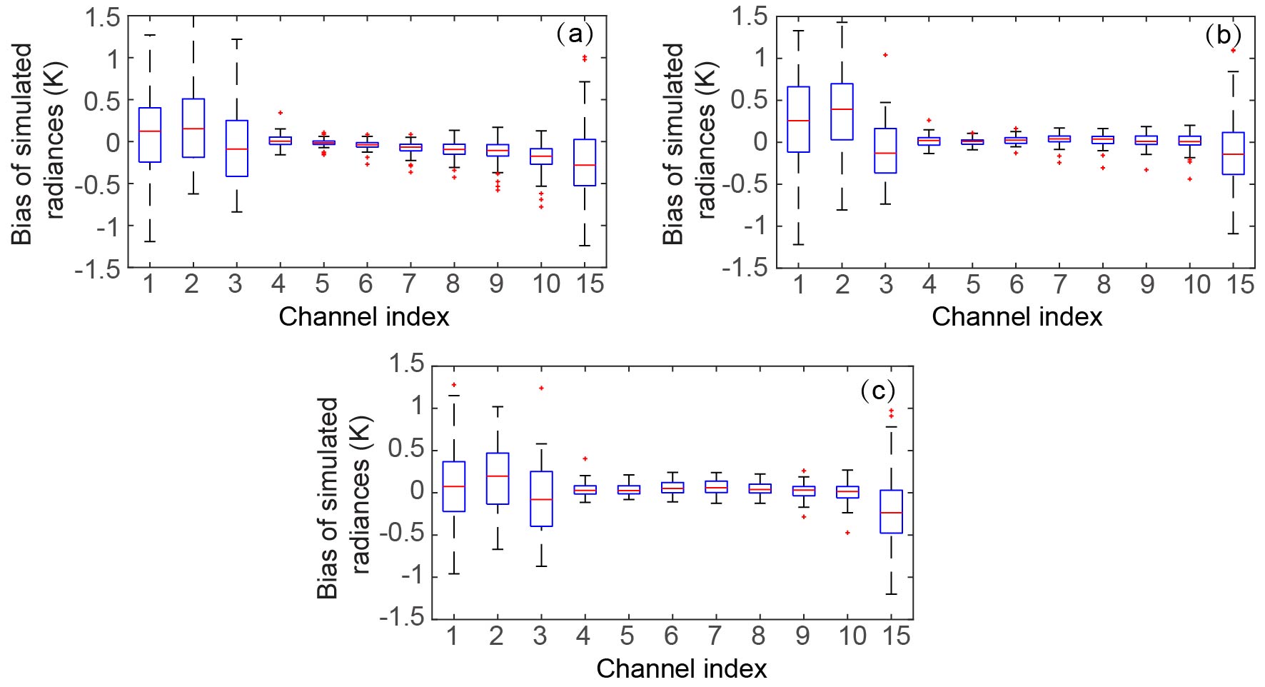Figure5. Boxplot of the bias of simulated radiances for NOAA-15 AMSU-A of the nine-day test period for experiments (a) EnKF_AMSUA_VarB, (b) EnKF_AMSUA_EnB and (c) EnKF_AMSUA_VarB_SP.


To see if only the radiance observations should be used to update $\,{\beta }$, EnKF_AMSUA_VarB_SP was conducted and the mean bias is presented in Fig. 5c. For channels 4?7, the box of mean biases of EnKF_AMSUA_VarB_SP appears much thicker than that of EnKF_AMSUA_VarB. This indicates that, for most analysis times, the former may have larger biases. To see this more clearly, we show the mean bias during the assimilation cycle for two selected channels in Fig. 6. In both channels, EnKF_AMSUA_EnB has the smallest mean bias among the three experiments. Running GSI variational bias correction with pure radiance observation does not reduce the mean bias. Instead, for channel 5, EnKF_AMSUA_VarB_SP even gets higher bias than EnKF_AMSUA_VarB (Fig. 6b), suggesting conventional datasets should not be excluded when updating bias correction coefficients. The difference between two bias correction methods may lie in the minimization procedure. It appears that the EnKF-based method, which uses optimal estimation, is less affected by available samples. The variational method, which uses a conjugate gradient algorithm, is more likely subjected to large bias in cases of small samples.
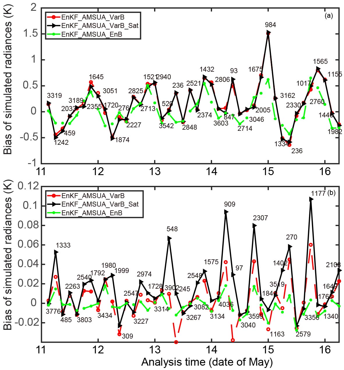Figure6. Bias of the simulated radiances for NOAA-15 AMSU-A (a) channel 2 and (b) channel 5. The numbers are the available observations during the bias correction procedure. The x-axis marks the date of the test period. For example, “11” represents 0000 UTC 11 May 2010.


The contributions of each predictor in both bias correction schemes are also compared, in Fig. 7. The black solid lines represent the total bias correction—that is, ${{P}^{\rm{T}}}{\beta }$ in Eq. (1). The red solid lines are the scan-angle component, which is updated outside GSI, while other dashed colored lines represent individual predictor terms for the online bias correction. In general, the behaviors of both experiments are very similar and both are stable in the recycled run. For most channels, the scan-angle component is a larger term. As we explained in section 2c, it represents the mean bias of each scan angle and is applied before the variational bias correction. Therefore, it is unsurprising to see relatively large values. For most channels, the global offset is also a large term and is comparable to the scan-angle term. These two predictors contribute to a great fraction of the total bias correction. In more recent versions of GSI, the scan-angle and air-mass steps are combined into one. In that case, the global offset term turns out to be the largest term for most channels (Zhu et al., 2014).
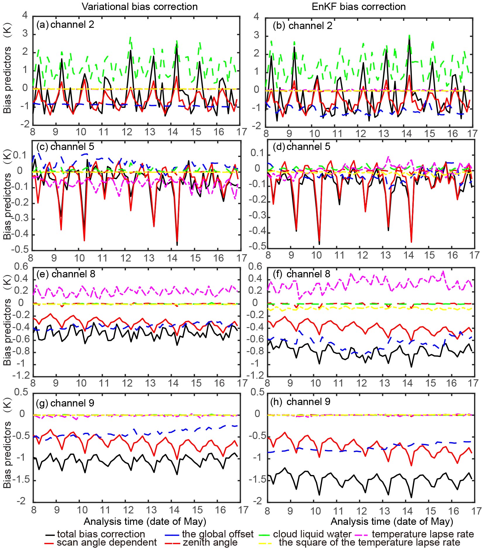Figure7. Time series of each predictor through the nine-day period. Panels (a, c, e, g) are from experiment EnKF_AMSUA_VarB for NOAA-15 AMSU-A channels 2, 5, 8 and 9, respectively. Panels (b, d, f, h) are similar to (a, c, e, g) but for experiment EnKF_AMSUA_ EnB.


For other predictors, their contributions vary channel by channel. For surface channel 2, the CLW dominates the variation of total bias correction (Figs. 7a and b). The contribution of CLW decreases rapidly with height for the upper-level channels 8 and 9 (Figs. 7e-h), and becomes zero through the nine-day period. Since CLW is not channel-dependent, the reduced impact indicates less correlation between CLW and the bias of upper-level channels. In contrast, the TLR term plays an increasingly important role in bias correction for channels 5 and 8 (Figs. 7c-f). The TLR term turns to zero at channel 9, which is consistent with the result of using standard US sounding profiles (see section 2). For higher-level channels, such as channel 11, TLR is again a key bias correction term (not shown).
The spatial distribution of predictors is given in Fig. 8. Here, we select surface channel 2 from experiment EnKF_AMSUA_EnB at 0000 UTC 13 May 2010 as an example (results from EnKF_AMSUA_VarB are similar and not shown here). The scan-angle component depends on the scan position and usually has larger bias for points at two edges than at the field of view (Fig. 8a). For the global offset term, its values are the same for all observation points in the same channel (not shown). The contribution of the zenith angle predictor is mostly small (Fig. 8b), consistent with Fig. 7, where the contributions of the zenith component are almost zero. The CLW term is currently only applied to satellite sensors at microwave frequency over oceans and under clear-sky conditions. Therefore, it is either zero or small for most points. The larger-value points indicate areas with rich water vapor but without precipitation or thick clouds (Fig. 8c) (Zhu et al., 2014). For TLR, as explained above, this is small for surface channel 2 (Fig. 8d). The square of TLR is nearly zero in this case and not shown. In short, the CLW term, which depends on the water vapor content, has considerable spatial variation and plays an important role in reducing biases for the low-level channels. The scan-angle component removes the mean bias of each scan position and is a large term for most channels (see also Fig. 7).
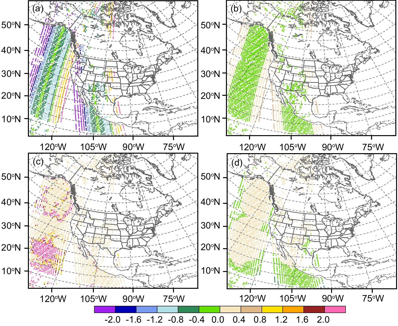Figure8. Values of each predictor (units: K) for NOAA-15 AMSU-A surface channel 2 at 0000 UTC 13 May 2010. The result of EnKF_AMSUA_ EnB is presented. The predictors are (a) the scan-angle component, (b) the zenith angle, (c) cloud liquid water, and (d) the temperature lapse rate. The global offset predictor is constant for all the points and is therefore not shown. The square of the temperature lapse rate predictor is nearly zero and is also not shown.


In Fig. 9, the RMSEs of experiments using the two different bias correction procedures, together with no satellite radiance assimilation, are displayed. The corresponding RPIs are also added. Considering that the EnKF system needs about three days to reach a stable stage, the first three days are excluded in Fig. 9 during the calculation of RMSEs and RPIs. In general, the RMSEs of experiments from assimilating AMSU-A radiance observations are lower than the no-radiance experiment for most variables and times except for temperature and RH during the first few hours. The corresponding RPIs indicate that the AMSU-A radiance assimilation significantly improves U and V forecasts at the 90% confidence level. For the two bias correction procedures, the RMSEs of EnKF_AMSUA_EnB are slightly lower than those of EnKF_AMSUA_VarB for RH, but are comparable for other variables. Their overall differences are not significant.
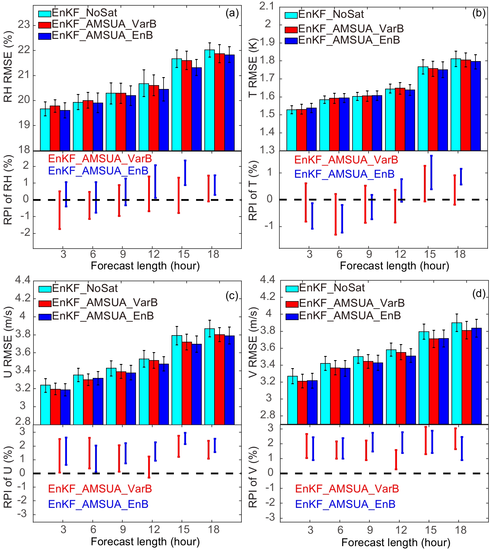Figure9. Domain-averaged forecast RMSEs verified against sounding observations (top panel in each subfigure), with error bars representing two-tailed 90% confidence intervals, and the RPIs calculated at the 90% confidence interval (bottom panel in each subfigure) for experiments with radiance assimilation compared to the no-satellite-radiance experiment EnKF_NoSat for (a) RH, (b) temperature, (c) U-wind, and (d) V-wind. The x-axis is the forecast hour. Only forecasts after the first three days are included in the statistics.


Overall, both variational and EnKF procedures have comparable performance and can effectively remove radiance biases. Using either variational or EnKF procedures, the AMSU-A radiance assimilation improves the forecast accuracy for most variables and times. In the following section, the full radiance datasets are assimilated. Both procedures show positive impact with additional radiance assimilation. The experiment with variational bias correction shows slightly better performance than that with EnKF-based bias correction for U and V. Similar to the AMSU-A tests, their differences are not significant. Therefore, for brevity, only the results using variational bias correction are presented in the next section. Another reason for choosing variational bias correction is that it is also used in the Hybrid EnKF system, which is currently under investigation.

2

-->

5.1. Assimilation of full radiance datasets using EnKF

Using the variational bias correction procedure with the recycled initial guess of ${{\beta }_{\rm{b}}}$, the full set of radiance data, including AMSU-A, AIRS, HIRS3/4 and AMSU-B, are assimilated in experiment EnKF_ALL. It can be seen that the assimilation of satellite radiance data reduces forecast error for most variables at most times (Fig. 10). The corresponding RPIs indicate that the improvements from assimilating radiance observations are significant for most variables and times at the 90% confidence level. Among the forecast variables and experiments, the largest improvement is achieved with the assimilation of radiance data using EnKF for variable RH. Compared to assimilating AMSU-A radiance alone, full radiance assimilation significantly improves the RH forecasts, as indicated by unanimously larger-than-zero RPIs, while for the experiment with only AMSU-A radiance assimilation the lower bounds are still below zero (see Fig. 9a). A preliminary investigation shows that this improvement is mostly contributed by AIRS radiance DA from 600 hPa to 300 hPa (not shown). For temperature, the positive impact is only seen after nine hours (Fig. 10b). For the horizontal wind vector, the positive impacts of radiance data are seen throughout the forecasts (Figs. 10a, c and d).
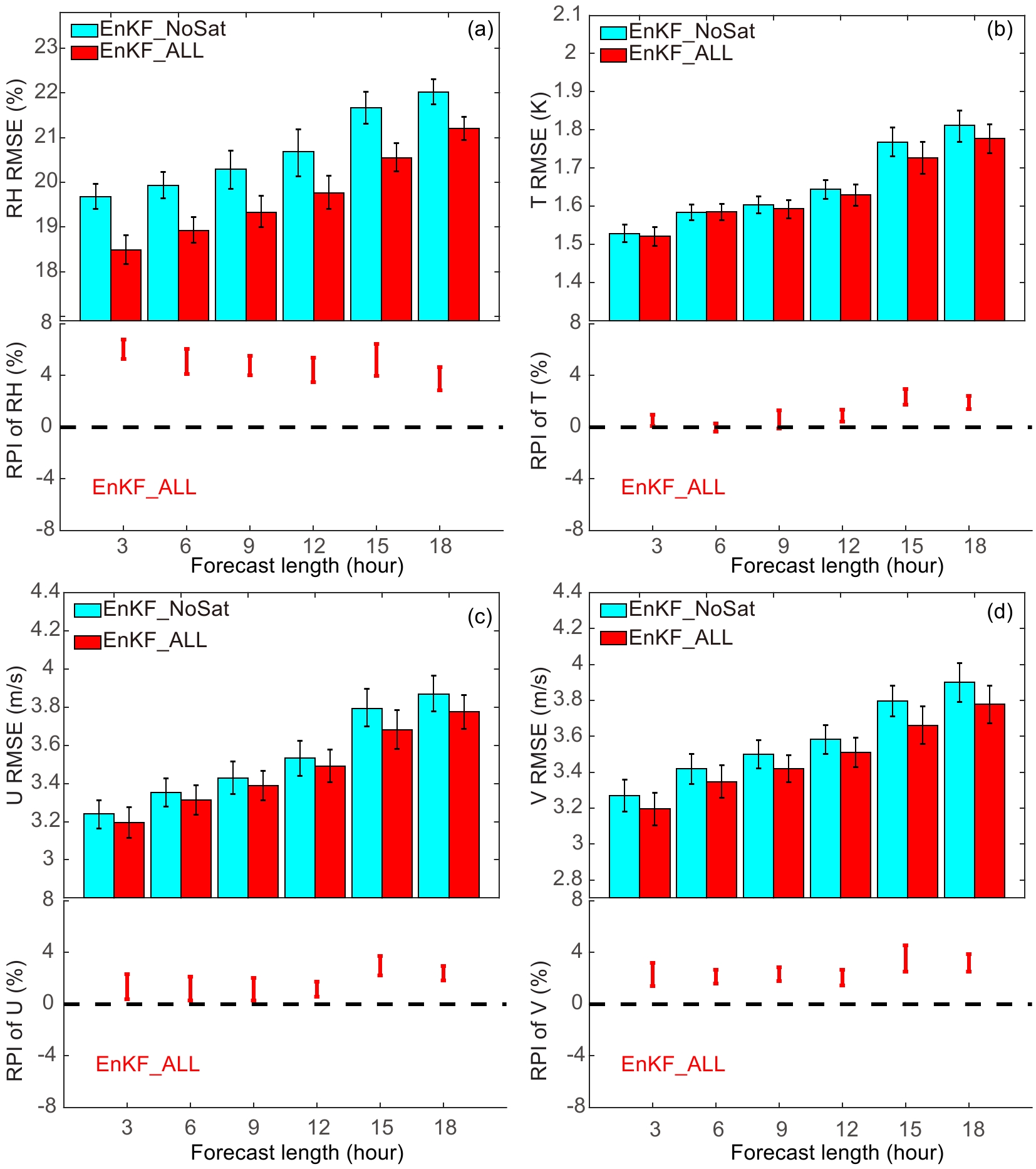Figure10. Domain-averaged forecast RMSEs verified against sounding observations (top panel in each subfigure), with error bars representing two-tailed 90% confidence intervals, and the RPIs calculated at the 90% confidence interval (bottom panel in each subfigure) for experiment EnKF_ALL compared to the no-satellite-radiance experiment EnKF_NoSat for (a) RH, (b) temperature, (c) U-wind, and (d) V-wind. The x-axis is the forecast hour. Only forecasts after the first three days are include in the statistics.


Figure 11 presents the mean 18-h forecast RMSEs at different heights for EnKF_ALL, and the corresponding experiment without satellite data. The RPIs comparing EnKF_ALL against EnKF_NoSat are also included. The assimilation of radiance data reduces the RMSEs at 18 hours for most variables and vertical levels. The RPIs at various levels are predominantly positive except for temperature. Most improvements are found at mid-levels between 600 and 300 hPa where RPI bounds at the 90% confidence level of EnKF_ALL are mostly greater than zero. This is because many channels peak at the mid-levels (Fig. 1), which also have less bias. In comparison, radiance data at lower levels are more easily contaminated by surface emissivity, while at higher levels some radiance channels are above the model top (Kazumori, 2014). Therefore, the values of RPIs are relatively small at lower and higher levels within our experiments.
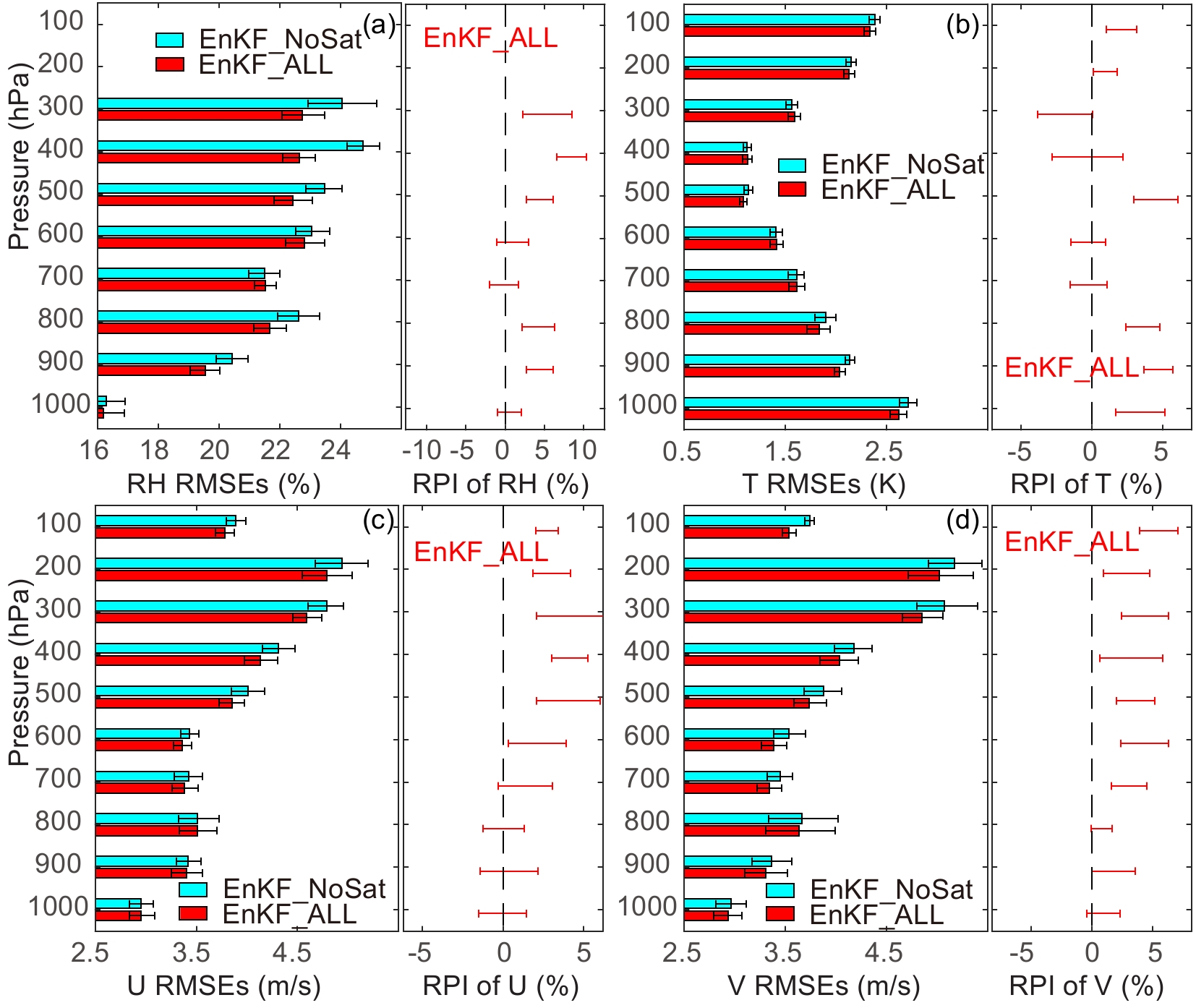Figure11. Mean 18-h forecast RMSEs at different heights for full-satellite and no-satellite-data experiments, verified against upper-air sounding data for (a) RH, (b) temperature, (c) U-wind, and (d) V-wind. Error bars represent two-tailed 90% confidence intervals using the bootstrap distribution method. The corresponding RPIs relative to the experiment without satellite data are plotted to the right of the RMSEs, with error bars indicating the 90% confidence interval. Only forecasts after the first three days are included in the statistics.


The surface forecast variables are verified against surface observations and are shown in Fig. 12 for hours 3 through 18. Unlike the assimilation of conventional data (including surface observations), radiance data have little direct impact on the analysis of surface variables. Yet, in our EnKF_ALL tests, almost all surface forecast variables show small but consistent improvements, except for surface pressure and 10-m U for the first 12 hours of forecasts. The RPIs are predominantly positive except for 10-m U. It is possible that observations from other sensors have compensated the AMSU-A radiance distribution at lower levels.
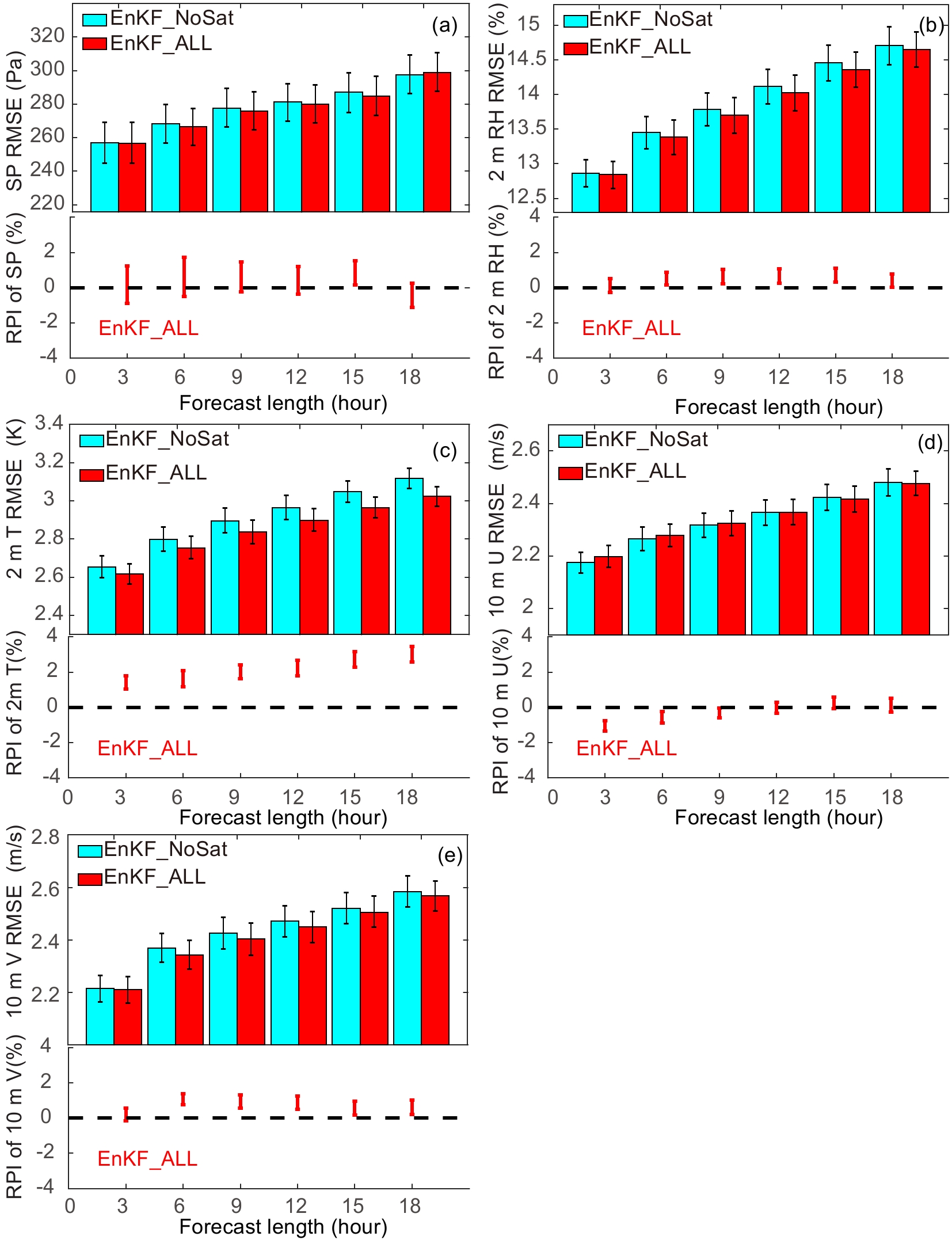Figure12. Domain-averaged forecast RMSEs verified against surface observations (top part of each subfigure) and RPIs calculated at the 90% confidence interval of experiment EnKF_ALL compared to the corresponding no-satellite-radiance experiment EnKF_NoSat for (a) surface pressure, (b) 2-m RH, (c) 2-m temperature, (d) 10-m U-wind, and (e) 10-m V-wind. The x-axis is the forecast hour. The error bars represent the two-tailed 90% confidence intervals. Only forecasts after the first three days are included in the statistics.



2 -->

5.2. Precipitation forecast skill on a 13-km grid

Two sets of forecasts are run on the 13-km grid, initialized from the interpolated 40-km grid analyses of EnKF_ALL and EnKF_NoSat, respectively. For convenience, these names are also used for the corresponding 13-km grid forecast experiments. Note that the no-satellite-data experiment (EnKF_NoSat) differs from experiment EnKF_CtrHDL of Z13 because of the addition of GPS PW data.
Figure 13 shows the GSSs and FBIAS over all forecasts starting from 0000 UTC 11 May to 1200 UTC 16 May 2010, for thresholds of 0.1 and 5.0 mm h^?1. Both scores are calculated from aggregated contingency tables. For the 0.1 mm h^?1 threshold, forecasts initialized from EnKF analyses show small but mostly positive impacts of satellite data in terms of GSSs. The FBIAS values of forecasts are larger than 1. However, for the 5.0 mm h^?1 threshold, the FBIAS values of all four experiments are less than 1 for the first six hours of forecasts, but close to 1 after that. The low FBIAS in the first six hours is due to model spin-up. With a better location of the water vapor transport belt, forecasts initialized from EnKF analyses in EnKF_ALL produce higher GSSs than EnKF_NoSat.
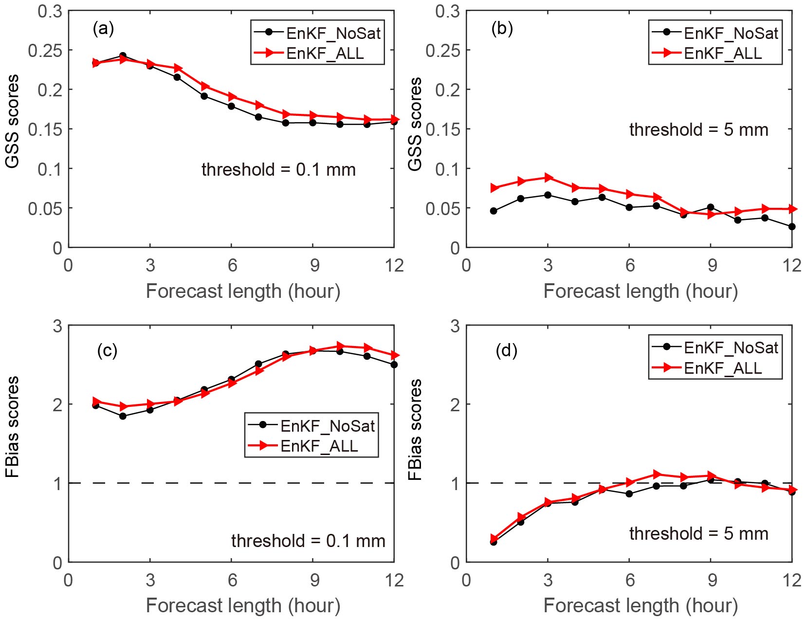Figure13. Aggregate hourly precipitation GSSs of all 13-km forecasts at different forecast lengths for thresholds at (a) 0.1 mm h^?1 and (b) 5.0 mm h^?1. (c, d) Corresponding frequency bias scores. Only forecasts after the first three days are included in the statistics.


Figure 14 presents the observed (top row) and 1-h accumulated precipitation forecast from EnKF_NoSat (middle row) and EnKF_ALL (bottom row) ensemble mean analyses. The left-hand column starts from 1200 UTC 11 May 2010 and the right-hand column from 1200 UTC 12 May 2010. For both cases, the assimilation of radiance data improves short-range precipitation forecasts. The forecast rain intensity in EnKF_ALL is closer to that of observations than that in EnKF_NoSat. For the second case, the predicted location of the rainstorm center is also more accurate. Since the 1-h forecasts are dominated by the initial condition, the positive contribution is mainly from radiance assimilation, which improves the RH analyses (Fig. 10a).
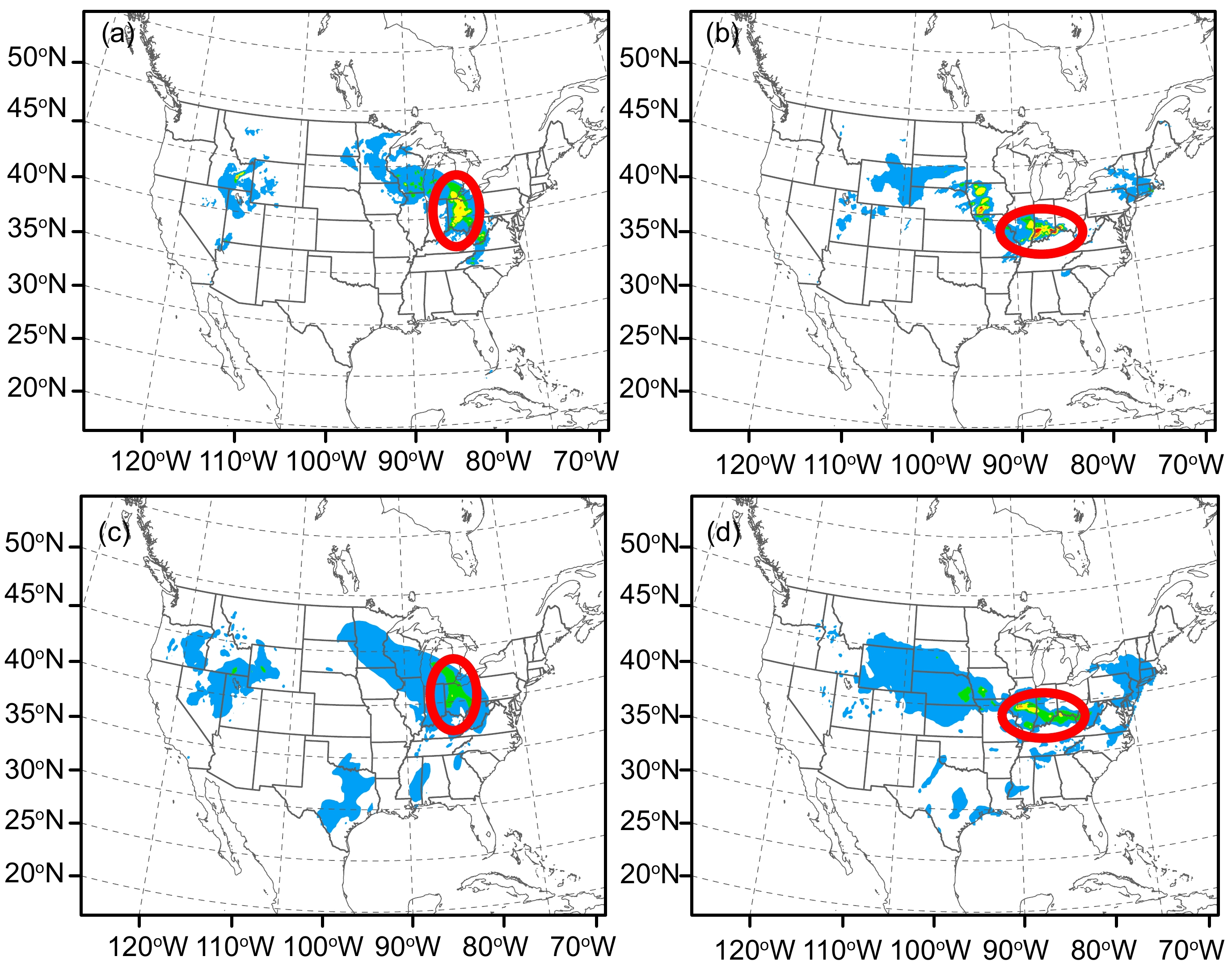Figure14. Observed and forecast 1-h accumulated precipitation (units: mm h^?1) for select forecasts starting from two different times: (a, b) NCEP stage IV precipitation; (c, d) forecasts from EnKF_NoSat analyses; (e, f) forecasts from EnKF_ALL analyses. The two sets of forecasts started at (left-hand column) 1200 UTC 11 May and (right-hand column) 1200 UTC 12 May 2010, respectively. Both are 1-h forecasts. The red circles indicate the locations of the most significant improvements.

In this study, satellite radiance data are assimilated within three-hourly assimilation cycles through a regional EnKF DA system established in Z13. All experiments are performed at 40-km grid spacing and have 40 ensemble members. Following Z13, the same nine-day test period starting from 8 May 2010 is used. Results are evaluated based on RMSEs of 3–18-h forecasts against upper-air sounding and surface observations.
The variational bias correction scheme within the GSI-3DVar system is first tested and compared with an EnKF bias correction scheme suitable for ensemble DA, using the AMSU-A data that have the best spatial coverage among all satellite data types. Both procedures effectively reduce the differences between observed and simulated radiances. In term of RMSEs, both procedures show similar performance and their differences are small and not significant at the 90% confidence level. In both experiments, short-range forecast accuracies are improved for most investigated variables and times, especially for upper-air wind components. In short, the EnKF and variational bias correction schemes have comparable performance.
Experiments assimilating the full set of radiance data, including AMSU-A, AMSU-B, AIRS, HIRS 3/4 and MHS, are then conducted using a common variational procedure. The results are compared with the experiment without radiance assimilation. The impacts of the radiance data are positive for most forecast variables, forecast times and height levels, especially for RH, when verified against sounding data. Additionally, as in Z13, deterministic forecasts are initialized on a 13-km grid at 0000 and 1200 UTC each day from the interpolated 40-km analyses. In terms of GSSs, precipitation is generally better predicted in experiments with radiance assimilation.
Finally, we point out again that the choice of a nine-day period for the assimilation experiments was limited by both the available computing resources, and by the available data (saved shortly after the real-time experimental RAP forecasts). The relatively short nine-day period might limit the effectiveness of the bias-correction coefficient estimation. For this reason, we implemented a recycling procedure of bias correction, where the coefficients estimated at the end of the nine-day DA cycles are used as the first guess at the beginning of repeated nine-day DA cycles. Results show that such recycling is beneficial to improving the results of the earlier DA cycles and the bias correction by the end of the first nine-day DA cycles is stabilized. In fact, the correction coefficients are found to be more or less stable after five to seven days within the first pass. We note here that, in operational implementations where the DA cycles run continuously, such a recycling procedure is not needed. With the recycling, our results are not affected much by the relatively short nine-day test period.
Acknowledgments. This work was primarily supported by the National Key Research and Development Program of China (Grant No. 2018YFC1507604) and the Special Foundation of the China Meteorological Administration (Grant No. GYHY201506006). This work was also supported by the National Science Foundation of China (Grant No. 41405100).