HTML
--> --> -->The coupled general circulation models (CGCMs) of phase 3 of the Coupled Model Intercomparison Project (CMIP3) have obtained diverse results in reproducing the observed ENSO–EASR relationship (Fu et al., 2013). Fu et al. (2013) analyzed the historical climate simulation of 18 CMIP3 CGCMs and found that only five of them realistically captured the ENSO–EASR relationship. Moreover, these five CGCMs seriously overestimated ENSO’s interannual variability and simulated the strongest interannual variabilities in TIO SST and PSC, indicating that an overestimated ENSO interannual variability is a precondition for successfully representing the three physical processes in CMIP3 CGCMs.
Fortunately, the ENSO–EASR relationship can be captured more reasonably in the CGCMs of phase 5 of CMIP (CMIP5) (Fu and Lu, 2017). Compared with less than one-third (5 out of 18) of the CMIP3 models, approximately two-thirds (14 out of 22) of the CMIP5 models capture a significant and more realistic ENSO–EASR relationship. This progress was due to the successful reproduction of the physical processes underpinning the relationship between ENSO and EASR, particularly the teleconnection between ENSO and TIO SST and the teleconnection between TIO SST and PSC. However, large intermodel diversity still exists, and the ENSO–EASR relationship is weaker than observed in most CMIP5 models.
Recently, the outputs of the latest generation of CGCMs, in phase 6 of CMIP (CMIP6), have begun to be released (Eyring et al., 2016), and it has already been found that CMIP6 CGCMs offer some improvements over their CMIP5 versions. For example, Fu et al. (2020) found that CMIP6 models exhibit remarkable progress in simulating the spatial characteristics of the zonal wind climatology at 200 hPa over East Asia, such as the location and intensity of the East Asian westerly jet core. Additionally, they also reveal improved interannual variability in the meridional displacement of the westerly jet over East Asia and its relationship with EASR.
Accordingly, we assess the ability of CMIP6 models to capture the ENSO–EASR relationship, and examine whether they offer any kind of progress compared with CMIP3 and CMIP5 models. Furthermore, we also evaluate the skills of CMIP6 models in reproducing the underlying physical processes, to determine their limitations in simulating this relationship.
Section 2 describes the data and methods. Section 3 presents the simulated ENSO–EASR correlation in the CMIP6 models and compares it with those in CMIP3 and CMIP5 models. Section 4 reports the results of simulating the aforementioned three key processes in the CMIP6 models, and compares them with those based on the CMIP3 and CMIP5 models. Section 5 sets out our conclusions and provides some further discussion.
| Model | Affiliation and country | Resolution |
| BCC-CSM2-MR | BCC, China | 320 × 160 |
| BCC-ESM1 | BCC, China | 128 × 64 |
| CAMS-CSM1-0 | CAMS, China | 320 × 160 |
| CanESM5 | CCCma, Canada | 128 × 64 |
| CESM2 | NCAR, USA | 288 × 192 |
| CESM2-WACCM | NCAR, USA | 288 × 192 |
| CNRM-CM6-1 | CNRM-CERFACS, France | 256 × 128 |
| CNRM-ESM2-1 | CNRM-CERFACS, France | 256 × 128 |
| FGOALS-g3 | IAP, China | 180 × 80 |
| GFDL-ESM4 | NOAA GFDL, USA | 288 × 180 |
| HadGEM3-GC31-LL | MOHC, UK | 192 × 144 |
| IPSL-CM6A-LR | IPSL, France | 144 × 143 |
| MCM-UA-1-0 | UA, USA | 96 × 80 |
| MIROC-ES2L | MIROC, Japan | 128 × 64 |
| MIROC6 | MIROC, Japan | 256 × 128 |
| MPI-ESM1-2-HR | MPI-M, Germany | 384 × 192 |
| MRI-ESM2-0 | MRI, Japan | 320 × 160 |
| NESM3 | NUIST, China | 192 × 96 |
| NorCPM1 | NCC, Norway | 144 × 96 |
| UKESM1-0-LL | MOHC, UK | 192 × 144 |
Table1. Basic information of the CMIP6 models used in this study.
The CMIP3 and CMIP5 models, methods and indices are identical to those used in previous studies (Fu et al., 2013; Fu and Lu, 2017). Briefly, the December–February (DJF) Ni?o3 index is defined as the DJF SST averaged over (5°S–5°N, 150°–90°W); the tropical Indian Ocean index (TIOI) is defined as the JJA SST averaged over (20°S–20°N, 40°–110°E); the Philippine Sea convective index (PSCI) is defined as the JJA precipitation averaged over (10°–20°N, 110°–160°E); and the EASR index (EASRI) is defined as the JJA precipitation averaged over the parallelogram-shaped region determined by the following points: (25°N, 100°E), (35°N, 100°E), (30°N, 160°E), and (40°N, 160°E).
 Figure1. Lead–lag correlation coefficients between the monthly Ni?o3 index and the JJA EASRI in the observations (1979–2019), CMIP6 MME, and individual CMIP6 models (1901–2014). The correlation coefficient shown in each subfigure was calculated between the observed curve and individual model curve. The horizontal dashed line illustrates the significant value at the 5% level. The left-hand vertical dashed line denotes January in the preceding winter; the right-hand vertical dashed line and the red triangle denote the lag-0 time, i.e., July in the subsequent summer.
The spatial patterns of wintertime ENSO-related JJA precipitation in the observations, CMIP6 MME, and individual CMIP6 models are shown in Fig. 2. The regressions were also calculated for individual models first, then the MME was calculated. In the observations, a positive wintertime ENSO event favors a remarkable above-normal EASR anomaly and a prominent below-normal precipitation anomaly over the Philippine Sea and northwestern subtropical Pacific. In the CMIP6 MME, the ENSO-related precipitation anomalies are weaker than the observations, both along the EASR belt and over the Philippine Sea. For the individual models, it is found that 14 models generally simulate the ENSO-related summer precipitation anomalies, indicated by the positive spatial correlation coefficients of approximately 0.24–0.54 between the observations and simulations. In the meantime, the precipitation anomalies are almost impossible to detect in some models (e.g., MCM-UA-1-0). Therefore, 11 out of 20 CMIP6 models realistically capture the temporal evolution of the lead–lag relationship between ENSO and EASR (Fig. 1), as well as the spatial characteristics of the ENSO-related precipitation anomalies (Fig. 2).
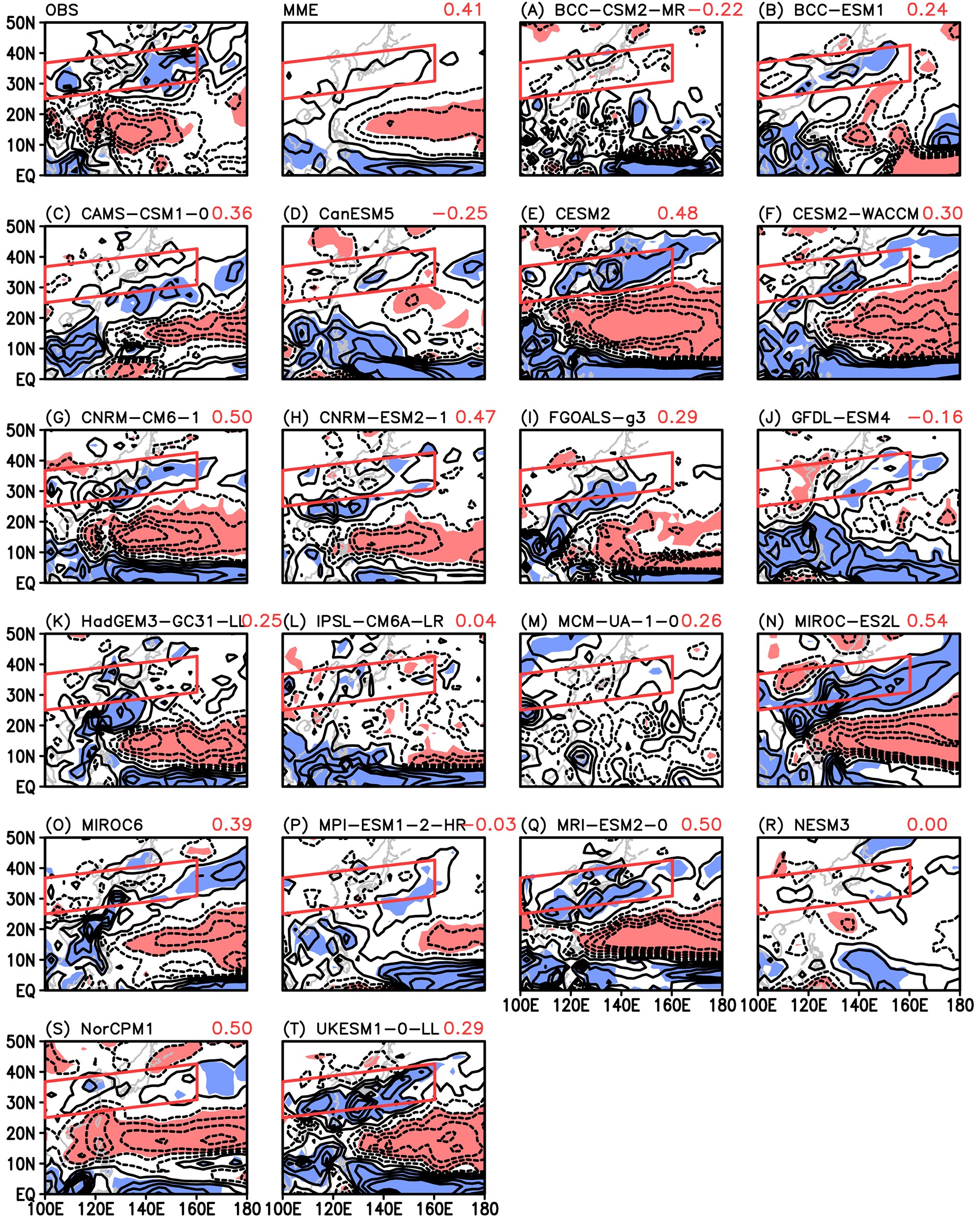 Figure2. The JJA precipitation regressed onto the standardized preceding DJF Ni?o3 index in the observations, CMIP6 MME, and individual CMIP6 models. Values significant at the 5% level are shaded (blue, positive; red, negative). The contour interval is ±0.1, ±0.3, ±0.5, ±0.7, and ±0.9, and the zero contour lines have been removed. The red parallelograms indicate the region used to define the EASRI. The spatial correlation coefficients between the observations and simulations are given in the top-right corners of each sub-plot. units: mm d?1.
To compare the ENSO–EASR relationship clearly in the three generations of models, the ENSO-related summer precipitation anomalies in the CMIP3 MME, CMIP5 MME, and CMIP6 MME are shown in Figs. 3a–c, respectively. The spatial patterns and intensities of the precipitation anomalies are similar in the three MMEs. The negative precipitation anomalies over the Philippine Sea and northwestern subtropical Pacific are gradually stronger from the CMIP3 MME to the CMIP6 MME. Otherwise, all three MMEs simulate positive precipitation anomalies over the equatorial western Pacific that do not exist in the observations. In the meantime, in order to clearly show the difference of magnitude and spatial distribution between the simulations and observations, the biases of ENSO-related JJA precipitation anomalies in the CMIP3, CMIP5, and CMIP6 MMEs are given in Figs. 3d–f. The biases of the summer precipitation anomalies are almost the same in terms of the spatial pattern and intensity in the CMIP3, CMIP5, and CMIP6 models. There are negative biases over central China and the western North Pacific that east of Japan in the three MMEs, with a maximum of approximately ?0.4 mm d?1, indicating weaker precipitation anomalies than observed. A weak positive bias of approximately 0.1 mm d?1 appears over the lower reaches of the Yangtze River valley and the East China Sea. The biases are positive and much larger over the Philippine Sea and tropical western Pacific, with a maximum of over 1.0 mm d?1, indicating stronger precipitation anomalies than observed.
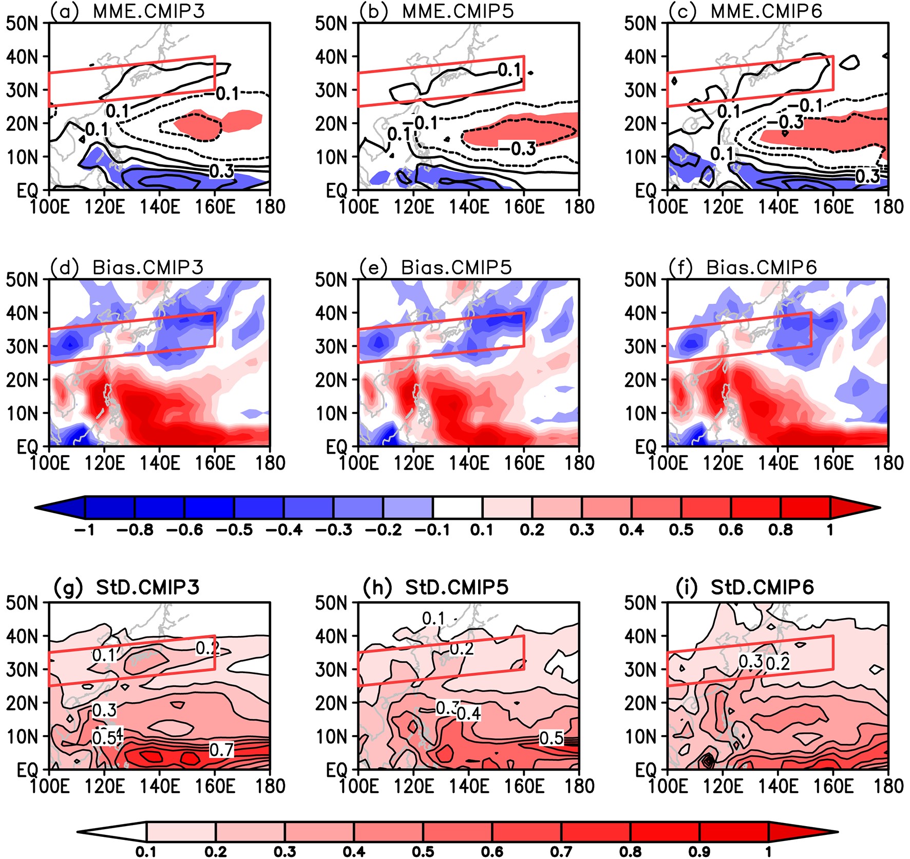 Figure3. (a–c) The JJA precipitation regressed onto the standardized preceding DJF Ni?o3 index in the CMIP3 MME, CMIP5 MME, and CMIP6 MME, respectively. Panel (a) is a reproduction of the MME result shown in Fig.2 in Fu et al. (2013), and (b) is a reproduction of the MME result shown in Fig.2 in Fu and Lu (2017). Values significant at the 5% level are shaded (blue, positive; red, negative). The contour interval is ±0.1, ±0.3, ±0.5, ±0.7 and ±0.9, and the zero contour lines have been removed. (d–f) The biases of the ENSO-related summer precipitation in the CMIP3 MME, CMIP5 MME, and CMIP6 MME (blue, weaker than observed; red, stronger than observed). (g–i) The intermodel standard deviations of the ENSO-related summer precipitation among the individual CMIP3, CMIP5, and CMIP6 models. The contour interval in (d–i) is 0.1. The red parallelograms indicate the region used to define the EASRI. Units: mm d?1.
Furthermore, in order to quantitatively evaluate the intermodel diversity in simulating the ENSO–EASR relationship, the intermodel standard deviation (StD) of the simulated ENSO-related summer precipitation anomalies among the individual models is also analyzed (Figs. 3g–i). The three generations of models exhibit similar spatial distributions of intermodel differences over the EASR region. The StD is approximately 0.1–0.3 mm d?1 over the rain belt among the CMIP3 models, and decreases to 0.1–0.2 mm d?1 among the CMIP5 models. A maximum locates over southern Japan and also decreases from approximately 0.3 mm d?1 to 0.2 mm d?1. The intermodel diversity over the EASR region in the CMIP6 MME is almost the same as that in the CMIP5 models. The results indicate a larger intermodel spread in the ENSO-related EASR anomaly among the CMIP6 models than among the CMIP5 models, and a smaller spread than among the CMIP3 models.
The distributions of the correlation coefficients between ENSO and EASR in the three generations of models are further shown in Fig. 4a, which is a duplicate of Fig. 3 in Fu and Lu (2017) but with the results of the CMIP6 models added. The correlation coefficients are stronger in the CMIP5 and CMIP6 models than in the CMIP3 models. In the meantime, the correlation coefficient is weaker in the CMIP6 models than in the CMIP5 models (Fig. 4a). The correlation coefficients have a peak percentage of approximately 33% between 0 and 0.10 in the CMIP3 models, 27% between 0.20 and 0.30 in the CMIP5 models, and 25% between 0.10 and 0.20 in the CMIP6 models. In addition, 10 out of 20 CMIP6 models, which successfully represent the temporal evolution and spatial pattern of ENSO’s impact on EASR, simulate significant ENSO–EASR relationships that are statistically significant at the 5% level, except for BCC-ESM1, which has a correlation coefficient of approximately 0.18.
 Figure4. (a) Distribution of correlation coefficient between the simulated preceding DJF Ni?o3 index and subsequent JJA EASRI in the CMIP3 (blue bars), CMIP5 (green bars), and CMIP6 (red bars) models. The figure is a reproduction of Fig. 3 in Fu and Lu (2017) but with the results of the CMIP6 models added. (b) Boxplot of ENSO–EASR correlation coefficients in the CMIP3, CMIP5, and CMIP6 models. The line in the box indicates the median value, the multiplication sign indicates the MME, and dots indicate the individual models. The observed value is given in the top-right corner.
Furthermore, the correlation coefficients between the DJF Ni?o3 index and EASRI show a larger spread in the CMIP6 models than in the CMIP5 models, and both are narrower than that in the CMIP3 models (Fig. 4b). The dispersion is ?0.16 to 0.77 in the CMIP3 models, ?0.06 to 0.55 in the CMIP5 models, and ?0.12 to 0.62 in the CMIP6 models. Between the 25th and 75th quartiles, the correlation coefficient changes from approximately 0.03 to 0.38 in the CMIP3 models, from 0.08 to 0.35 in the CMIP5 models, and from 0.08 to 0.30 in the CMIP6 models. The MME and median value of the ENSO–EASR correlation coefficient are both approximately 0.20 in the CMIP6 models, which are weaker than those in the CMIP5 models (0.23 and 0.24) and stronger than those in the CMIP3 models (0.19 and 0.11). Additionally, the ENSO–EASR correlation coefficients are weaker than the observed value (0.44) in almost all the CMIP3, CMIP5, and CMIP6 models.
In summary, the CMIP6 models show progress in capturing the ENSO–EASR correlation compared with the CMIP3 models. However, the CMIP6 models bear a number of similarities to the CMIP5 models in terms of reproducing the ENSO–EASR relationship, suggesting almost no distinct progress in reproducing this relationship.
2
4.1. Simulation of the relationship between ENSO and TIO SST
Figure 5 shows the subsequent-summer TIO SST regressed onto the standardized DJF Ni?o3 index in the observations, CMIP6 MME, and individual CMIP6 models. Generally, there are three SST anomaly centers in the observations, located over the northwestern Indian Ocean, southwestern Indian Ocean, and southeastern Indian Ocean. Except for BCC-ESM1 and MCM-UA-1-0, all CMIP6 models reproduce the SST anomaly related to ENSO over the Indian Ocean, especially over the northern TIO where the SST anomaly plays a more important role in affecting the western North Pacific circulation (Xie et al., 2009; Huang et al., 2010). Most CMIP6 models fail to capture the SST anomaly over the southeastern Indian Ocean. In contrast, the ENSO-related TIO SST anomaly can be simulated in only half of the CMIP3 models (Fu et al., 2013), but it can be represented in almost all CMIP5 models, even in the “worst” CMIP5 models that have the weakest ENSO–EASR relationships (Fu and Lu, 2017). On the other hand, there is a positive SST anomaly over the eastern tropical Pacific in the observations, which is consistent with previous studies (e.g., Xie et al., 2009). Almost all the CMIP6 models represent this SST anomaly with stronger intensity than observed. In the meantime, most models simulate negative SST anomalies over the southern tropical Pacific, which do not exist in the observations. It seems that the simulated SST anomaly over the tropical Pacific cannot directly affect the ENSO–EASR relationship. Figure5. As in Fig. 2 but for the JJA SST regressed onto the standardized DJF Ni?o3 index. Values significant at the 5% level are shaded (red, positive; blue, negative), and the contour interval is 0.05. Units: °C.
The MMEs of the three generations of models simulate almost the same spatial pattern and intensity of ENSO-related TIO SST anomalies (Figs. 6a–c). The MMEs successfully represent the ENSO-induced SST anomalies over the northwestern and southwestern Indian Ocean, but cannot reproduce the SST anomaly over the southeastern Indian Ocean. The biases of the simulated SST anomalies between the CMIP models and the observations are positive over the tropical western Indian Ocean and central southern TIO (Figs. 6d–f), indicating an overestimation compared with the observations. Additionally, the biases are negative over the southeastern Indian Ocean in the MMEs because of the unsuccessful representation of the observed positive SST anomaly in the models.
 Figure6. As in Fig. 3 but for the JJA SST regressed onto the standardized DJF Ni?o3 index. Panel (a) is a reproduction of the MME result shown in Fig.4 in Fu et al. (2013). Shading in (a–c) indicates values significant at the 5% level (red, positive; blue, negative). The contour interval is 0.05 in (a–c) and 0.02 in (d–i). Units: °C.
The intermodel diversity of the ENSO-related SST anomaly decreases from the CMIP3 to CMIP6 models (Figs. 6g–i). In the CMIP3 models, the intermodel StDs reach up to approximately 0.16–0.18°C over the northwestern, southwestern, and southeastern Indian Ocean. In the CMIP5 models, the largest intermodel diversity is still located over these regions, but the StDs decrease to approximately 0.10–0.12°C. In the CMIP6 models, the intermodel diversity centers over the southern TIO almost disapper, with the StDs decreasing to only approximately 0.06–0.08°C. The center over the northwestern TIO also shrinks and decreases to approximately 0.10°C. Additionally, the intermodel StD over the central Indian Ocean decreases from approximately 0.10°C in the CMIP3 models to 0.04°C in the CMIP6 models.
The improvement in the CMIP6 models in simulating ENSO’s impact on TIO SST is clearly shown in Fig. 7a, which is a reproduction of Fig.5a in Fu and Lu (2017) but with the results of the CMIP6 models added. The correlation coefficients between ENSO and TIOI tend to be stronger and are nearer to the observations (0.66) in the CMIP6 models compared with those in the CMIP3 and CMIP5 models. The correlation coefficients are within 0.70–0.80 in the largest percentage of CMIP6 models (50%), and range from 0.80 to 0.90 in the following proportion (20%). That is, 70% of the CMIP6 models simulate the ENSO–TIOI correlation coefficient within 0.70–0.90, which are stronger than the observed values. The percentage is much greater compared with that in the CMIP3 models (39%) and CMIP5 models (59%). Additionally, the correlation coefficients are stronger than 0.60 in approximately 50% of the CMIP3 models, 68% of the CMIP5 models, and 85% of the CMIP6 models.
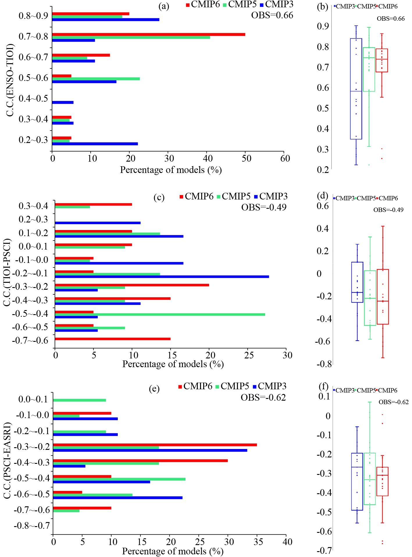 Figure7. As in Fig. 4 but (a, b) the correlation coefficient between the preceding DJF Ni?o3 index and TIOI, (c, d) the TIOI–PSCI correlation coefficient, and (e, f) the PSCI–EASRI correlation coefficient. Panels (a, c, e) are reproductions of Figs. 5a-c in Fu and Lu (2017) but with the results of the CMIP6 models added.
The CMIP6 models exhibit smaller dispersion in the ENSO–TIOI correlation coefficients than the CMIP3 and CMIP5 models (Fig. 7b). There are only two outliers (BCC-ESM1 and MCM-UA-1-0) that simulate much lower correlation coefficients (approximately < 0.30). The correlation coefficient ranges from approximately 0.22 to 0.90 in the CMIP3 models, 0.31 to 0.90 in the CMIP5 models (except for one outlier), and from 0.55 to 0.86 in the CMIP6 models (except for two outliers). Between the 25th and 75th quartiles, the correlation coefficients are within the scope of approximately 0.35–0.84 in the CMIP3 models and 0.58–0.79 in the CMIP5 models, and the scope narrows to 0.67–0.79 in the CMIP6 models. Additionally, the MMEs of the correlation coefficients are approximately 0.59, 0.68, and 0.69 in the CMIP3, CMIP5, and CMIP6 models, respectively; and the median values are approximately 0.58, 0.74, and 0.74.
Based on the above results, we can conclude that the CMIP6 models simulate the ENSO–TIOI relationship more reasonably than the CMIP3 and CMIP5 models.
2
4.2. Simulation of the relationship between TIO SST and PSC
Figure 8 shows the JJA precipitation regressed onto the standardized TIOI, which represents the second step of ENSO’s impact on EASR. In the observations, a positive TIO SST anomaly corresponds to a below-normal rainfall anomaly over the Philippine Sea and northwestern subtropical Pacific. This negative TIOI-related precipitation anomaly is successfully represented in the CMIP6 MME and 12 out of 20 CMIP6 models (CAMS-CSM1-0, CESM2, CESM2-WACCM, CNRM-CM6-1, CNRM-ESM2-1, FGOALS-g3, HadGEM3-GC31-LL, MCM-UA-1-0, MIROC-ES2L, MRI-ESM2-0, NorCPM1, and UKESM1-0-LL). The ratio is nearly identical to that in the CMIP5 models (12 out of 22) (Fu and Lu, 2017) and greater than that in the CMIP3 CGCMs (5 out of 18) (Fu et al., 2013). The negative precipitation anomaly in MIROC6 is relatively weak and shifts far eastward in comparison with the observations (Fig. 8o), resulting in an insignificant TIOI–PSCI correlation coefficient of approximately 0.18. Otherwise, the main body of the TIOI-related negative precipitation anomaly shifts eastward by approximately 20° in longitude compared with the observations, with the western edge located east of 130°E in six CMIP6 models (CAMS-CSM1-0, CESM2-WACCM, FGOALS-g3, HadGEM3-GC31-LL, MCM-UA-1-0, and UKESM1-0-LL).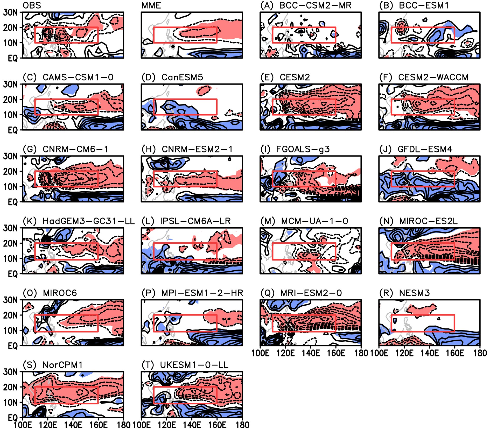 Figure8. As in Fig. 2 but for the JJA precipitation regressed onto the standardized TIOI. The red rectangles indicate the region used to define the PSCI. Units: mm d?1.
More importantly, the well-simulated TIOI–PSCI relationship guarantees that the CMIP6 models will capture the ENSO–EASR correlation, which is quite different from the CMIP5 models. Except for MCM-UA-1-0 and NorCPM1, all the remaining 10 CMIP6 models that capture a significant TIOI–PSCI relationship of between ?0.24 and ?0.74 are models that realistically simulate the ENSO–EASR relationship. The two exceptions have TIOI–PSCI correlation coefficients of approximately ?0.24 and ?0.55, but the ENSO–EASR correlation coefficients are only 0.12 and 0.10, respectively. All remaining eight CMIP6 models that cannot reproduce the significant TIOI–PSCI relationship fail to capture the ENSO–EASR relationship. On the other hand, all 10 CMIP6 models that simulate a significant ENSO–EASR relationship are also models that realistically represent a significant TIOI–PSCI relationship. However, this phenomenon does not exist in the CMIP5 models, and no obvious connection can be found between the TIOI–PSCI and ENSO–EASR correlations (Fu and Lu, 2017).
The TIOI-related precipitation anomaly over the Philippine Sea and northwestern subtropical Pacific in the CMIP6 MME is relatively stronger than those in the CMIP3 and CMIP5 MMEs (Figs. 9a–c). It also shows that the simulated PSC shifts eastward in all three MMEs, with the western edge located east of 130°E. Accordingly, the biases, with the maximum located over 120°–140°E, decrease from the CMIP3 to CMIP5 models (Figs. 9d–f). Different from the MMEs and biases, the intermodel spread in the CMIP6 models, however, increases. Over the PSC region, the intermodel StDs are approximately 0.2–0.3 mm d?1 in the CMIP3 models (Fig. 9g), 0.3–0.4 mm d?1 in the CMIP5 models (Fig. 9h), and larger than 0.4 mm d?1 in the CMIP6 models (Fig. 9i).
 Figure9. As in Fig. 3 but for the JJA precipitation regressed onto the standardized TIOI. Panel (a) is a reproduction of the MME result shown in Fig.7 in Fu et al. (2013). The contour interval is 0.2 in (a–f) and 0.1 in (g–i). The red rectangles indicate the region used to define the PSCI. Units: mm d?1.
Figure 7c displays a histogram of the TIOI–PSCI correlation coefficients in the CMIP3, CMIP5, and CMIP6 models, which is a reproduction of Fig.5b in Fu and Lu (2017) but with the results of the CMIP6 models added. Generally, the intensity of the TIOI–PSCI correlation coefficients in the CMIP5 and CMIP6 models exhibit almost no obvious difference, and they are both stronger than that in the CMIP3 models. In the largest percentage of the CMIP6 models (20%), the correlation coefficients are within the scope of ?0.20 to ?0.30. In the CMIP5 models, the correlation coefficients of the largest proportion (27%) range from ?0.50 to ?0.40, which is stronger than that in the CMIP6 models, while the correlation coefficients of the largest proportion (28%) are weaker, at only ?0.20 to ?0.10, in the CMIP3 models. Additionally, 60% of the CMIP6 models reasonably represent the TIOI–PSCI correlation coefficient (< ?0.20). The ratio is comparable to that in the CMIP5 models (55%) and larger than that in the CMIP3 models (28%).
Figure 7d quantitatively shows that the intermodel diversity increases from the CMIP3 to CMIP6 models. The scope of the TIOI–PSCI correlation coefficients is from approximately ?0.59 to 0.26 in the CMIP3 models, ?0.58 to 0.32 in the CMIP5 models, and increases to ?0.74 to 0.42 in the CMIP6 models. Between the 25th and 75th quartiles, the correlation coefficients change from approximately ?0.25 to 0.10 in the CMIP3 models, ?0.45 to 0.03 in the CMIP5 models, and ?0.44 to 0.04 in the CMIP6 models. The MME/median values are ?0.12/?0.17, ?0.21/?0.22, and ?0.21/?0.24 in the CMIP3, CMIP5, and CMIP6 models, respectively. Additionally, the observed TIOI–PSCI relationship (?0.49) is underestimated in almost all three generations of models.
In summary, the most important improvement is that the well-simulated TIOI–PSCI relationship guarantees that the CMIP6 models will realistically capture the ENSO–EASR correlation, but this is not the case in the CMIP5 models. However, the CMIP6 models show no obvious changes in terms of simulating this relationship. The TIOI–PSCI correlation coefficients in the CMIP6 models are almost the same as those in the CMIP5 models and stronger than those in the CMIP3 models.
2
4.3. Simulation of the relationship between PSC and EASR
Figure 10 shows the summer precipitation regressed onto the standardized PSCI in the observations, CMIP6 MME, and individual CMIP6 models. In the observations, a positive PSCI induces a negative EASR anomaly, which indicates a representation of the Pacific–Japan pattern (Lu, 2004; Kosaka and Nakamura, 2006). The below-normal precipitation anomaly is simulated in 18 out of 20 CMIP6 models (all except BCC-ESM1 and NESM3), although it is much weaker in most models than that in the observations. In contrast, 14 out of 18 CMIP3 models (Fu et al., 2013) and 17 out of 22 CMIP5 models (Fu and Lu, 2017) can represent the PSCI–EASRI relationship. Therefore, most CMIP models can reproduce the inherent relationships of the East Asian summer monsoon well. Figure10. As in Fig. 2 but for the JJA precipitation regressed onto the standardized PSCI. Units: mm d?1.
The intensity and spatial characteristics of the PSCI-related EASR anomaly are similar to each other in the MMEs, and all are much weaker than those in the observations (Figs. 11a–c). Accordingly, the biases of the precipitation anomaly in the MMEs exhibit nearly the same pattern and intensity (Figs. 11d–f). The positive biases are mainly located over central China and the Pacific that east of Japan. The intermodel diversity exhibits almost no difference from each other in the three generations of models, with intermodel StDs of approximately 0.2 mm d?1 over the EASR region (Figs. 11g–i). Therefore, the three generations of models have similar skills in representing the PSCI–EASRI relationship.
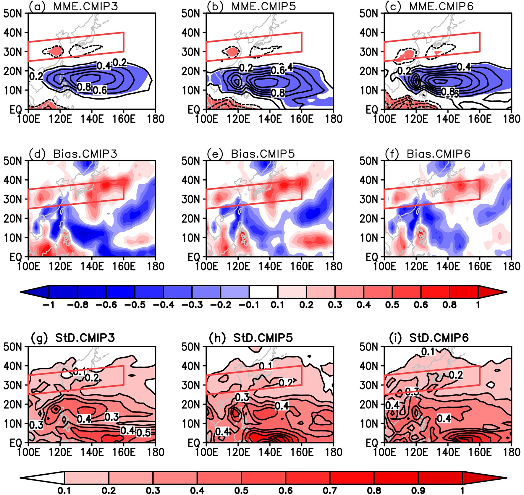 Figure11. As in Fig. 3 but for the JJA precipitation regressed onto the standardized PSCI. The contour interval is 0.2 in (a–f) and 0.1 in (g–i). Units: mm d?1.
Figure 7e shows that the PSCI–EASRI correlation coefficient tends to become weaker in the CMIP6 models, especially compared with that in the CMIP5 models. Approximately 90% of the CMIP6 models simulate a significant PSCI–EASRI relationship (< ?0.20) that is statistically significant at the 5% level. The ratio is slightly larger than that in the CMIP3 (78%) and CMIP5 (77%) models. However, strong correlation coefficients (< ?0.40) are simulated in only 25% of the CMIP6 models, which is lower than that in the CMIP3 (39%) and CMIP5 (41%) models. The correlation coefficients change from ?0.30 to ?0.20 with the peak proportion (35%) in the CMIP6 models, which is weaker than that of ?0.50 to ?0.40 (23%) in the CMIP5 models and identical to that of ?0.30 to ?0.20 (33%) in the CMIP3 models. Additionally, the PSCI–EASRI relationship is weaker than observed (?0.62) in almost all the analyzed CMIP3, CMIP5, and CMIP6 models.
Except for the outliers with correlation coefficients markedly stronger (MIROC-ES2L and UKESM1-0-LL) or weaker (BCC-ESM1 and NESM3) than those of the other models, the simulated PSCI–EASRI relationship tends to be more concentrated in the CMIP6 models than in the CMIP3 and CMIP5 models (Fig. 7f). The correlation coefficients spread from ?0.56 to ?0.21 in the CMIP6 models (except four outliers), while they range from ?0.56 to ?0.06 in the CMIP3 models and from ?0.61 to 0.07 in the CMIP5 models. Between the 25th and 75th quartiles, the correlation coefficients change from approximately ?0.50 to ?0.20 in the CMIP3 models, from ?0.46 to ?0.20 in the CMIP5 models, and from ?0.42 to ?0.27 in the CMIP6 models. Additionally, almost all three generations of models underestimate the PSCI–EASRI relationship.
In summary, the three generations of models exhibit essentially identical capabilities in representing the PSCI–EASRI relationship, with almost the same spatial pattern, intensity, bias, and intermodel diversity of the PSC-related precipitation anomaly. However, the correlation coefficient is weaker in the CMIP6 models, although it is more concentrated after excluding the outliers.
The above study evaluated the three physical processes related to the delayed impact of winter ENSO on the subsequent EASR in the CMIP6 models and compared the results with those in the CMIP3 and CMIP5 models. According to the analysis in section 4.2, except MCM-UA-1-0 and NorCPM1, all remaining 10 CMIP6 models that capture a significant TIOI–PSCI relationship are identical to the models that reproduce a significant ENSO–EASR relationship, and the eight CMIP6 models that cannot reproduce a significant TIOI–PSCI relationship fail to capture the ENSO–EASR relationship. This suggests that the TIOI–PSCI relationship is the key teleconnection determining whether the CMIP6 models can simulate the ENSO–EASR relationship. Unfortunately, the CMIP6 models fail to offer any improvement in simulating the TIOI–PSCI relationship, although they simulate a more realistic ENSO–TIOI relationship. The failure likely explains the fact that there is no obvious progress in simulating the ENSO–EASR relationship, as identified in section 3. Additionally, the ENSO–EASR relationship shows a slightly larger intermodel uncertainty in the CMIP6 models than in the CMIP5 models (Fig. 4b), which is attributable to the increased intermodel spread in the TIOI–PSCI relationship (Fig. 7d) since the intermodel spread for the remaining two physical processes is reduced (Figs. 7b and f). This result further supports the conclusion that the TIOI–PSCI relationship is the key process in determining the reproduction of the ENSO–EASR relationship in the CMIP6 models.
This study also investigates the three related physical processes through which ENSO affects EASR. The CMIP6 models simulate the effect of wintertime ENSO on the TIO SST in the following summer more reasonably than the CMIP3 and CMIP5 models. The realistic ENSO–TIOI correlation coefficients are stronger and captured by almost all CMIP6 models, with smaller intermodel dispersion, than those in the CMIP3 and CMIP5 models. However, there is almost no obvious difference in the simulated effect of summertime TIO SST on PSC, and the effect of PSC on EASR, between the CMIP5 and CMIP6 models. The TIOI–PSCI correlation coefficients in the CMIP6 models are nearly identical to those in the CMIP5 models, stronger than those in the CMIP3 models, and exhibit larger intermodel diversity. Additionally, most of the three generations of models capture the PSCI–EASRI relationship and exhibit essentially identical capabilities in representing the characteristics of the PSCI-related precipitation anomaly.
Further analysis indicates that almost all the CMIP6 models that capture a significant TIOI–PSCI relationship are models that realistically simulate the ENSO–EASR relationship. All the CMIP6 models that cannot reproduce a significant TIOI–PSCI relationship fail to capture the ENSO–EASR relationship. That is, the well-simulated TIOI–PSCI relationship guarantees that the CMIP6 models will realistically capture the ENSO–EASR correlation. However, on the other hand, a smaller ratio of the CMIP6 models capture the TIOI–PSCI relationship than the CMIP5 models. All the analyzed CMIP6 models simulate weaker teleconnection than observed, and exhibit almost no obvious improvement in representing the intensity of this physical process compared with the CMIP5 models. Therefore, improving the skill to realistically capture the TIOI–PSCI relationship is important for the next generation of CGCMs to reasonably obtain the ENSO–EASR relationship.
This study also shows that, from the CMIP3 to CMIP6 models, almost no obvious progress can be found in the simulation of the PSCI–EASRI relationship, although the CMIP6 models have been improved in many aspects (Wu et al., 2019; Wyser et al., 2019) and have better capability in simulating the East Asian summer monsoon (Fu et al., 2020). It also might be a challenge for the current CGCMs to simulate well the ENSO–EASR relationship. Therefore, further research should be undertaken to investigate the impact of PSC on EASR and to determine the reasons hindering models from representing well the inherent physical process.
Acknowledgements. We acknowledge the World Climate Research Programme, which, through its Working Group on Coupled Modelling, coordinated and promoted CMIP6. We thank the climate modeling groups for producing and making available their model output, the Earth System Grid Federation (ESGF) for archiving the data and providing access, and the multiple funding agencies who support CMIP6 and ESGF. This research was supported by the National Key R&D Program of China (Grant No. 2017YFA0603802), the Strategic Priority Research Program of the Chinese Academy of Sciences (Grant No. XDA2006040102), and the National Natural Science Foundation of China (Grant No. 41675084).
