Lei LIU¹,
Fei HU^1,2,,

Corresponding author: Fei HU,hufei@mail.iap.ac.cn

1.State Key Laboratory of Atmospheric Boundary Layer Physics and Atmospheric Chemistry, Institute of Atmospheric Physics, Chinese Academy of Sciences, Beijing 100029, China
2.University of Chinese Academy of Sciences, Beijing 100049, China
Manuscript received: 2019-02-20
Manuscript revised: 2019-05-06
Manuscript accepted: 2019-05-28
Abstract:In this paper, we use fluctuation analysis to study statistical correlations in wind speed time series. Each time series used here was recorded hourly over 40 years. The fluctuation functions of wind speed time series were found to scale with a universal exponent approximating to 0.7, which means that the wind speed time series are long-term correlated. In the classical method of extreme estimations, data are commonly assumed to be independent (without correlations). This assumption will lead to an overestimation if data are long-term correlated. We thus propose a simple method to improve extreme wind speed estimations based on correlation analysis. In our method, extreme wind speeds are obtained by simply scaling the mean return period in the classical method. The scaling ratio is an analytic function of the scaling exponent in the fluctuation analysis.
Keywords: extreme wind speed,
fluctuation analysis,
generalized Pareto distribution,
long-term correlation
摘要:风速的极值估计在风工程结构设计中具有广泛的应用。现有的极值估计方法假设风速时间序列中不存在统计相关特征。然而，真实的风速往往具有“聚团”现象，即较大的风速值往往聚集出现。“聚团”现象不存在于统计独立的时间序列中，表明风速时间序列存在明显的统计相关特征。本文利用起伏分析方法，分析了持续时间长达40年的9组小时风速历史记录。研究结果表明，风速时间序列的起伏指数均约等于0.7，大于统计独立时间序列的起伏指数0.5，证明了风速时间序列普遍具有长程统计相关的特征。因此，基于统计独立假设的传统方法对风速极值的估计必然存在偏差，而这一偏差体现在伴随长程相关特征出现的“聚团”现象，引起了平均回归时间与极值发生概率的关系出现偏差。本文通过数据分析，提出了长程相关风速时间序列极值的平均回归时间与极值发生概率的关系，并基于这一关系，提出了风速极值估计的新方法。这一方法可以通过一个简单的变换关系修正传统方法对风速极值的高估。
关键词:风速极值,
起伏分析,
长程相关,
广义Pareto分布

HTML

--> --> -->

Extreme wind speed estimation is an important procedure for designing various structures in wind engineering (Holmes, 2015). The classical method for estimating extremes from data is based on a mathematical theory of extreme statistics (Gumbel, 1958). A critical assumption of this theory is that data should have no or fast decaying correlations (Coles, 2001). However, wind speed time series are generally found to be long-term correlated (Santhanam and Kantz, 2005; Liu and Hu, 2013). In this case, the classical method would give an unreliable estimation of extreme wind speeds. New methods based on the mathematical theory of extreme statistics with long-term correlations and the long-term correlation characteristics of wind speeds are thus needed.
The mathematical theory of extreme statistics with long-term correlations is still developing, but the results already obtained are also helpful for understanding extreme characteristics and can give some clues to extreme estimations of long-term correlated series. One result shows that correlations would not affect the extreme distribution. This conclusion is evident to the POT extremes (i.e., peaks or values over a threshold). If a series is randomly shuffled, statistical correlations in this series will be destroyed but the POT extremes will not change. The situation is more complex for the block extreme (i.e., the maximum value during a fixed time period). A theorem states that the block extreme distribution of a stationary Gaussian sequence will converge to the Gumbel distribution as the time period increases to infinity, provided that the autocovariace $C\left( k \right){\rm{ln}}\left( k \right) \to 0$ for $k \to \infty $ (Berman, 1964; Leadbetter et al., 1983). The covariance between two observations of a time series x_i (i=1,2,…) with a mean μ, separated by k intervals of time, is called the autocovariance at lag k and is defined by $C\left( k \right) = {\rm{E}}\left[ {\left( {{x_{i + k}} - \mu } \right)\left( {{x_i} - \mu } \right)} \right]$. The Gumbel distribution is one of the three types of the generalized extreme value (GEV) distribution, which has been strictly proven to be obeyed in the case without correlations (Coles, 2001). Numerical simulations have shown that even for a long-term correlated time series with a non-Gaussian distribution and a power decay of $C\left( k \right)$, its block extreme distribution still converges to the GEV distribution (Eichner et al., 2006; Moloney and Davidsen, 2009; Schumann et al., 2012). The convergence rate is related to the distribution of series values (Eichner et al., 2006). Wind speeds are affected by many factors and their distribution varies from case to case. This is a reason why there is much debate on the choice of GEV types of wind speed extremes (Peterka and Shahid, 1998; Palutikof et al., 1999; Cook and Harris, 2004; Anastasiades and McSharry, 2014).
Another result states that extremes in a long-term correlated time series always appear in clusters (Bunde et al., 2005). As a result, the distribution of the extreme return period will deviate from the exponential distribution, which is obeyed in cases without correlations (Ross, 1996; Liu et al., 2014). Besides, the relation between the mean return period of extremes and the probability of extreme occurrences (hereafter called the T?P relation) becomes more complex. In this paper, we firstly analyze the long-term correlations of wind speed time series by fluctuation analysis (section 3.1). Then, a new T?P relation of extreme wind speeds is proposed (section 3.2). Here, we use the POT extreme because it is of greater utility and higher significance to climate time series compared to the block extreme (Ding et al., 2008), and it is also widely used in wind engineering (Holmes and Moriarty, 1999; Palutikof et al., 1999; Larsén et al., 2015). Finally, the classical extreme estimation method for series without correlations is briefly reviewed (section 4.1) and generalized to cases with long-term correlations (section 4.2).

Data used in this paper were collected from a database of the KNMI HYDRA Project, created by the Royal Netherlands Meteorological Institute. Nine hourly wind speed time series over 40 years were chosen for the following analysis (see Table 1). Wind speed values have been corrected for differences in measuring height and local roughness in the upstream sector (Wever and Groen, 2009). Missing data in the records were either interpolated by the cubic spine interpolation method, or just ignored if they appeared in the beginning of records.

Station	T0 (day/month/year)	Nm
Schiphol	1/3/1950	0
De Bilt	1/1/1961	1
Soesterberg	1/3/1958	4
Leeuwarden	1/4/1961	0
Eelde	1/1/1961	1
Vlissingen	2/1/1961	0
Zestienhoven	1/10/1961	4
Eindhoven	1/1/1960	1
Beek	1/1/1962	1

Table1. The KNMI HYDRA project data used in this paper. ${T_0}$ is the start time of data records and ${N_{\rm{m}}}$ is the number of missing data. All the data end at 31/12/2006.

2

-->

3.1. Fluctuation analysis

Autocovariance is a useful tool to describe statistical correlations in random time series. The autocovariance of a time series ${x_i}\left( {i = 1,2, \cdots ,N} \right)$ is defined by
where $\mu = {\rm{E}}\left[ {{x_i}} \right]$. If $C\left( k \right) \sim {k^{ - \gamma }}$ with $k \to \infty $ and $\gamma \in \left( {0,1} \right)$, the time series is referred to as long-term correlated (Beran, 1994). For long-term correlated time series, the autocovariance decays very slowly, and $\displaystyle\int_0^\infty {C\left( k \right){\rm{d}}k = \infty } $, which means that the area surrounded by the autocovariance curve and the axes is unlimited. For time series without correlations or with short-term correlations, the autocovariance decays much faster, and the area surrounded by the autocovariance curve and the axes is limited.
Generally, autocovariance calculated by Eq. (1) is more and more scattered with the increase of k. Thus, it is difficult to obtain a reliable estimation of γ by autocovariance analysis (Beran, 1994; Kantelhardt et al., 2001). Fluctuation analysis is a commonly used method to detect long-term correlations in time series (Peng et al., 1992). It can also give a better estimation of γ than the autocovariance analysis. Fluctuation analysis comes from a more general method named detrended fluctuation analysis (DFA). In DFA, trends in the cumulative summation of time series, obtained by fitting with a high-order polynomial, are eliminated (Peng et al., 1994). Very often, it is difficult to estimate the underlying trends in data, and inappropriate detrending could lead to artificial results (Kantelhardt et al., 2001). Besides, Bryce and Sprague (2012) pointed out that, in contrast to the mystery surrounding the action and interpretation of DFA, use of the fluctuation analysis method is straightforward and interpretable. In practice, wind trends are also interesting in many wind engineering applications. Thus, we do not detrend the data and only use fluctuation analysis in this paper.
Fluctuation analysis is described as follows. The path of a time series ${x_i}(i = 1,2, \cdots ,N)$ is defined by
where $m = 1,2, \cdots ,N$. The increment of the path with a time lag of s is
and its standard deviation F(s) is called the fluctuation function. If $F\left( s \right) \sim {s^\alpha }$ and $\alpha > 1/2 $ at large values of s, the time series is long-term correlated. The scaling exponent of the fluctuation function α is related to the scaling exponent of the autocovariance γ (Kantelhardt et al., 2001):
Figure 1 is a fluctuation analysis of the wind speed time series listed in Table 1. It shows that wind speed time series are long-term correlated because the values of α are evidently greater than 0.5 for all samples. We note that the scaling exponent of the fluctuation function seems to be universal for wind speed time series. Although observation time and sites vary in the samples, all the values of α approximate to 0.7.
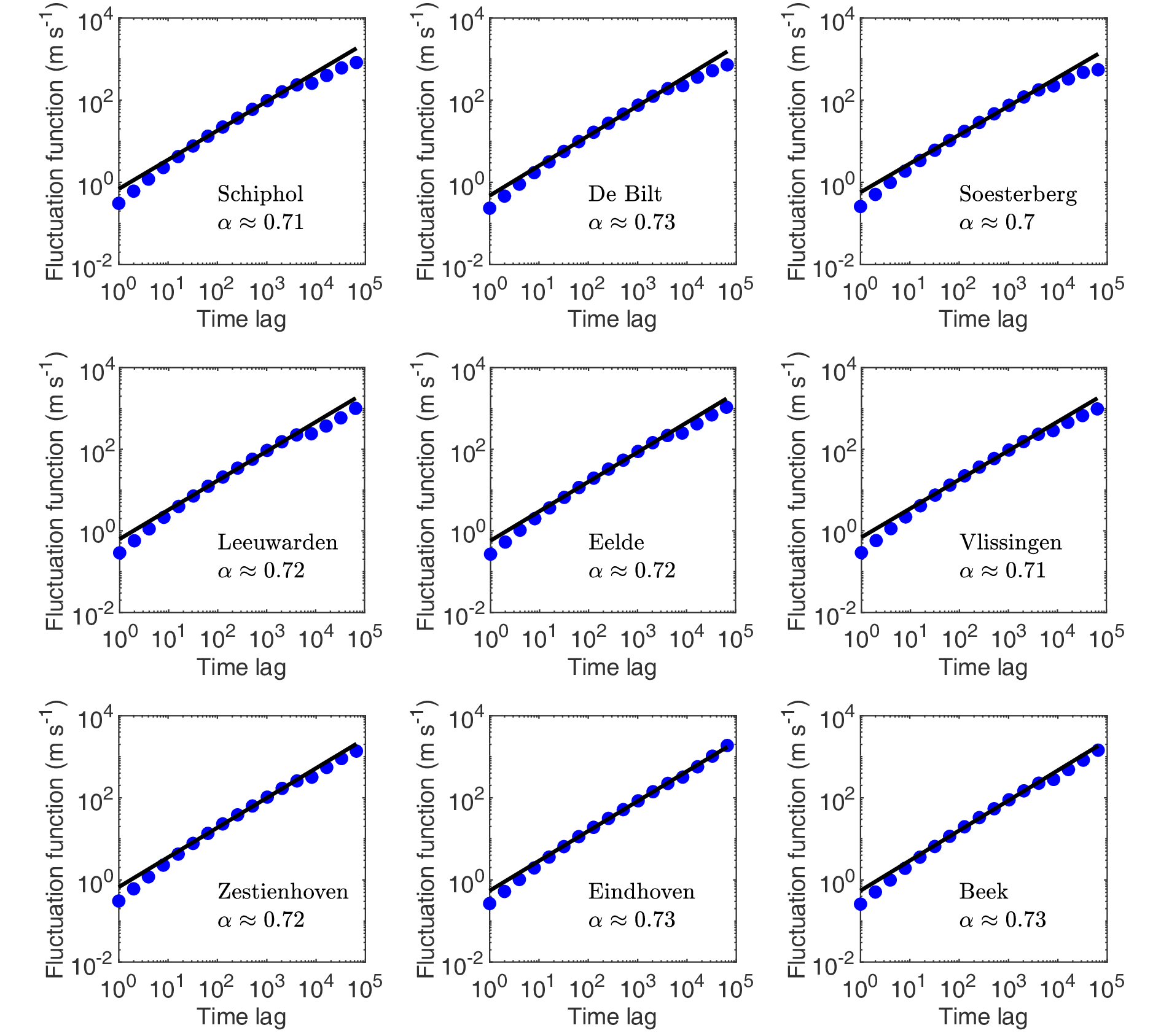Figure1. Fluctuation analysis of wind speed time series listed in Table 1. Lines are linear fittings in log-log plots, and the fitted scaling exponent of the fluctuation function $\alpha $ is also shown in each plot.



2 -->

3.2. The T?P relation

In this paper, the relation between the mean return period of extremes and the probability of extreme occurrences is called the T?P relation. This relation is critical for extreme estimations and is very different between cases with or without correlations. If the time series is assumed to be statistically independent (i.e., without correlations), the return periods of values greater than a threshold is exponentially distributed (Ross, 1996; Liu et al., 2014) and the corresponding T?P relation is derived by
where T is the mean return period, ?t is the sampling time, and P_z is the probability of values greater than a value of z.
Unlike cases without correlations, the return periods of POT extremes in long-term correlated time series will deviate from the exponential distribution. Figure 2 is an example of return period distributions of extreme wind speeds over different thresholds. Because the wind speed time series is long-term correlated (section 3.1), the data decay much slower than the exponential distribution (see the dashed line in Fig. 2). It was found that the so-called stretched exponential distribution can fit the data better (see the black line in Fig. 2). In fact, data analysis and numerical simulations have found that the stretched exponential distribution can fit return periods in various time series (Altmann and Kantz, 2005; Bunde et al., 2005; Santhanam and Kantz, 2005; Liu et al., 2014). Besides, we found that the statistics of return periods of extreme wind speeds can be simply normalized. If the return periods are normalized by their mean, the distributions with different thresholds will collapse into a single curve except for large values of return periods. The scattered tails may be caused by limited data.
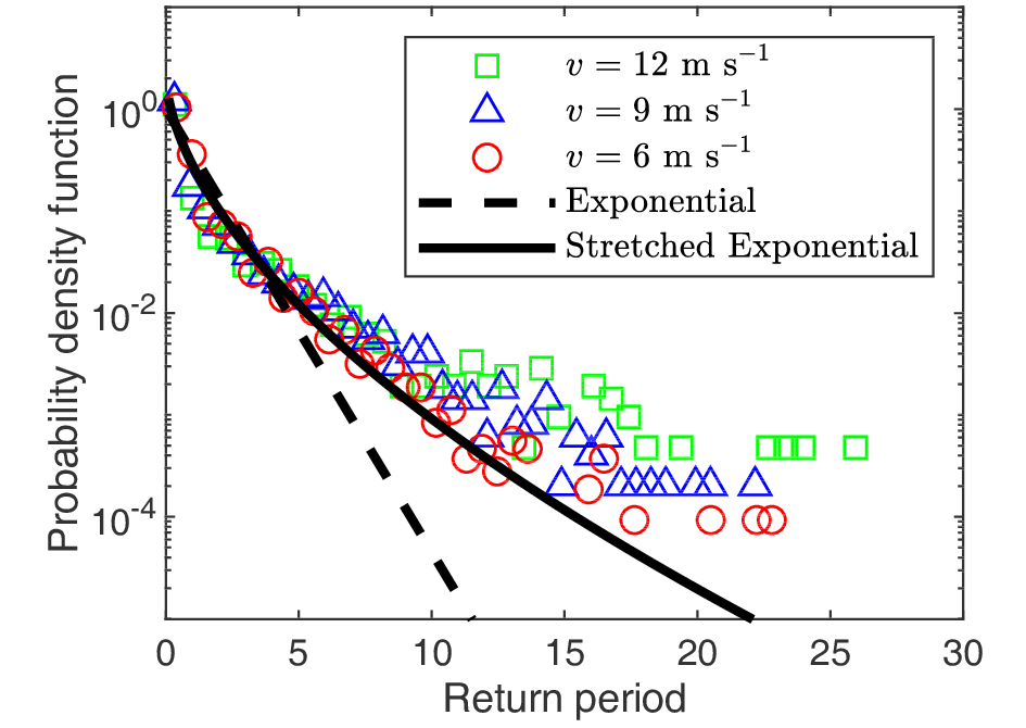Figure2. Probability density functions of return periods for wind speeds (the Schiphol data) greater than different thresholds of $v$. Note that the return period is divided by its mean. For comparison, the exponential distribution (dashed line) and the stretched exponential distribution (line) are also shown in this plot.


The stretched exponential distribution is defined by
where parameters a, b and $ \kappa $ are related by $ a = (b{\kappa })\bigr/\left[{{\varGamma \left( {1/\kappa } \right)}}\right]. $
If $\kappa = 1$, the stretched exponential distribution is exactly an exponential distribution. By numerical simulations and data analysis, it was found that $\kappa \approx \gamma $ (Bunde et al., 2005; Altmann and Kantz, 2005). It means that the parameter $ \kappa $ is also an indicator of statistical correlations. With Eq. (4), we have
In Fig. 2, the value of $ \kappa $ in the stretched exponential distribution is estimated by Eq. (7). The mean return period of the stretched exponential distribution is
where
Generally, the parameter b is a function of$ \kappa $ and P_z. In cases without correlations, $\kappa = 1$ and $b\left( {\kappa ,{P_z}} \right) = {P_z}/\Delta t$. This can be seen as a boundary condition of $b\left( {\kappa ,{P_z}} \right)$. In cases with long-term correlations, we simply assume that b is independent of $ \kappa $. Considering the boundary condition, we obtain $b\left( {{P_z}} \right) = {P_z}/\Delta t. $ Then, the T?P relation relation for long-term correlated series is
We found that Eq. (10) is indeed a good approximation of the T?P relation of extreme wind speeds (see Fig. 3). Besides, one can see that if the mean return periods are normalized by ${C_\kappa }\Delta t$, all the data will collapse into a single curve, as predicted by Eq. (10).
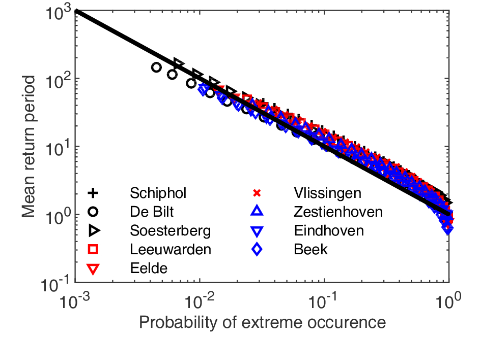Figure3. The T?P relation for wind speed time series listed in Table 1. Note that the mean return period is divided by ${C_\kappa }{\rm{\Delta }}t$, where the coefficient $C_\kappa$ is shown in Eq. (9) and $\Delta t$ is the sampling time. The line denotes a reciprocal function of the probability of extreme occurrences (see Eq. (10)).

A fraction of wind speed time series measured at Schiphol is plotted in Fig. 4a. The time series is then randomly shuffled (see Fig. 4b). The shuffled time series has no correlations but has the same distribution as the raw time series (Santhanam and Kantz, 2005; Liu et al., 2014). Comparing Fig. 4a and Fig. 4b, one can find that extremes in the long-term correlated wind speed time series appear in clusters, as stated by Bunde et al. (2005). If we set the same threshold in Fig. 4a and Fig. 4b (shown by dashed lines), it can be seen that the mean return period of POT extremes (i.e. peaks or values over a threshold) in raw data is larger than that of the shuffled data. It means that the extreme wind speeds will be smaller than those in the shuffled data with the same return period. That is to say, the classical method dealing with series without correlations would overestimate extreme wind speeds with long-term correlations. In this section, we propose a very simple method to improve extreme estimations in the long-term correlated wind speed time series.
Figure4. (a) The wind speed time series measured at Schiphol from 1 January 2005 to 31 December 2005. (b) The time series in (a) having been randomly shuffled. An arbitrarily chosen threshold is denoted by a dashed line in each panel.



2

-->

4.1. The classical method

The classical method dealing with series without correlations is briefly introduced here. More details can be referred to in the book by Coles (2001). The limiting conditional probability of POT extremes as the threshold $v$ increases is described by the generalized Pareto distribution (GPD),
where ${\rm{Pr}}\{ p|q\} $ denotes the probability of p with a condition q and the parameters $y \geqslant 0$, $\sigma > 0$ and $\xi \in \left( { - \infty ,\infty } \right)$. According to Eqs. (5) and (11), one can obtain the T-year return level; that is, the value expected to be exceeded once on average every T years:
where ${P_v} \equiv {\rm{Pr}}\{ V > v\} $ and l is a length of one year measured by the sampling time ?t. For example, if $\Delta t = 1\;{\rm{h}}$, $l = 365 \,\times \, 24 = 8760$.

2 -->

4.2. A new method with long-term correlations

As discussed in section 1, the limiting distribution of POT extremes as the threshold increases is the same whether or not the series is long-term correlated. Parameters in the GPD can be estimated by the maximum likelihood method (Coles, 2001). We compare the empirical conditional probabilities of extreme wind speeds with the GPD and find that the former is well described by the latter except for very large values (see Fig. 5). Deviations at large values would be caused by unreliable statistics of limited data. In practice, the threshold v is selected by a balance between bias and variance. If v is too low, the conditional probability cannot be well approximated by the GPD. If v is too large, the variance of parameters is large due to limited data. As far as we know, there is not a well-established method for the threshold selection (Scarrott and MacDonald, 2012). The commonly used upper 10% rule is just used here (DuMouchel, 1983). According to this rule, the threshold is defined to be the 90th percentile of samples. Table 2 lists the thresholds, the maximum likelihood estimations of GPD parameters and the corresponding confidence intervals.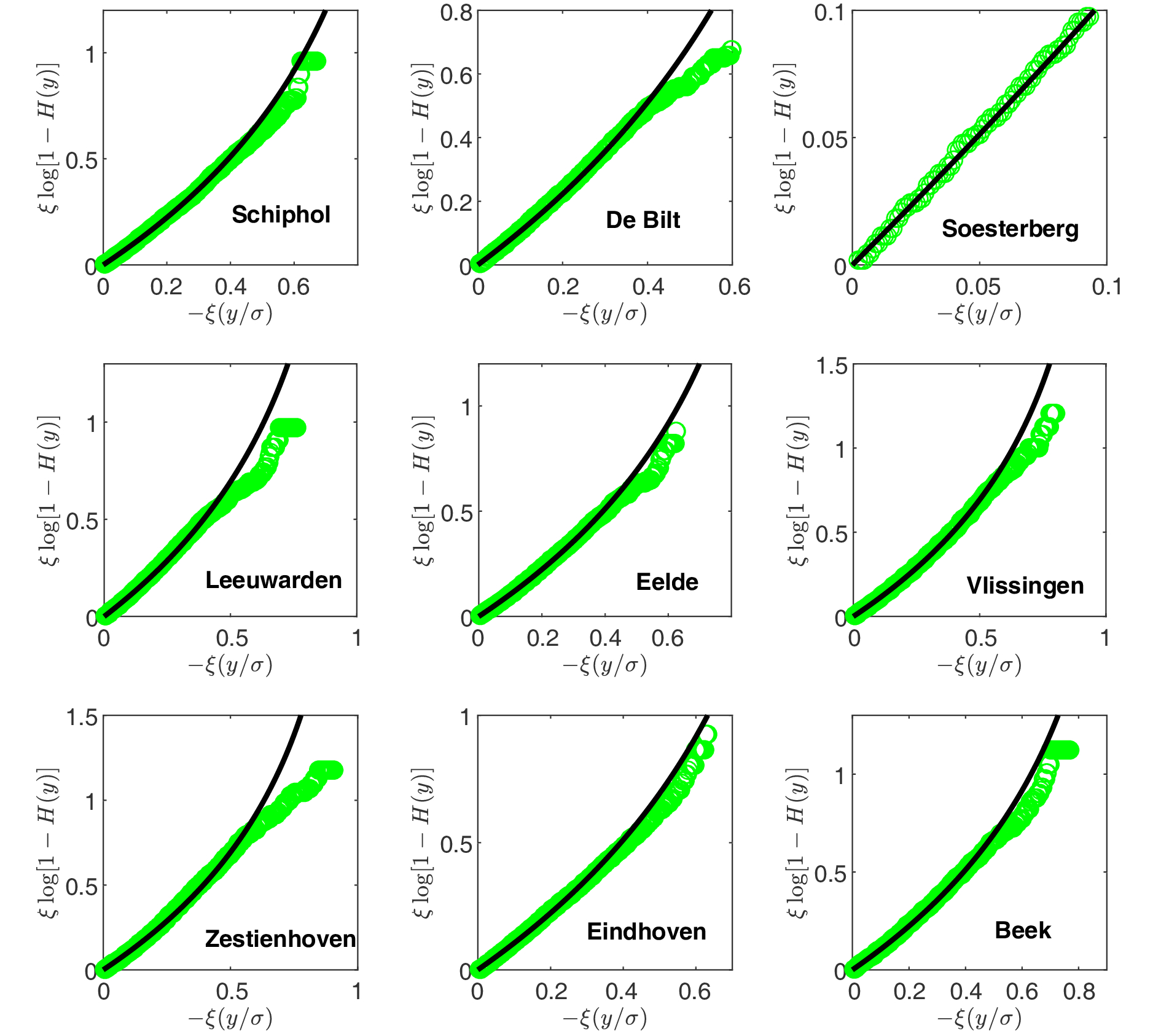
Figure5. Diagnostic plots of the GPD fittings to the wind speed time series listed in Table 1. Points show the empirical conditional probability of extreme wind speeds. Lines show the GPD with their parameters estimated by the maximum likelihood method (see Table 2)

Station	$v\;\left( {{\rm{m}}\;{{\rm{s}}^{ - 1}}} \right)$	$\xi$	${\rm{CI}}\left( \xi \right)$	$\sigma $	${\rm{CI}}\left( \sigma \right)$
Schiphol	9.5	?0.0893	(?0.0967, ?0.0819)	2.4566	(2.4282, 2.4854)
De Bilt	7.2	?0.0799	(?0.0876, ?0.0722)	1.8141	(1.7913, 1.8372)
Soesterberg	7.6	?0.0406	(?0.0491, ?0.0320)	1.7858	(1.7630, 1.8089)
Leeuwarden	9.1	?0.0921	(?0.0994, ?0.0848)	2.2890	(2.2609, 2.3175)
Eelde	8.3	?0.0831	(?0.0914, ?0.0748)	2.0926	(2.0658, 2.1198)
Vlissingen	9.5	?0.1142	(?0.1219, ?0.1066)	2.3182	(2.2893, 2.3474)
Zestienhoven	9.3	?0.1195	(?0.1249, ?0.1141)	2.3018	(2.2759, 2.3281)
Eindhoven	8.0	?0.0876	(?0.0957, ?0.0796)	2.1138	(2.0869, 2.1410)
Beek	8.1	?0.1065	(?0.1143, ?0.0987)	2.0573	(2.0314, 2.0836)

Table2. Thresholds $v$ and maximum likelihood estimations of the GPD parameters $\xi $ and $\sigma $. CI denotes the 95% confidence interval for the parameter estimated.


According to Eqs. (10) and (11), the T-year return level of long-term correlated wind speeds is calculated by
Comparing Eqs. (12) and (13), we have
The above equation states that the T-year return level of long-term correlated wind speeds can be simply obtained by just scaling the value of T in the classical method dealing with series without correlations. It means that the classical method, already implemented in many commercial software or open source programs, does not need to be discarded in cases with long-term correlations.
The procedure of the extreme wind speed estimations is illustrated in Fig. 6. For wind speed time series, α ≈ 0.7 (see Fig. 1). Thus, $\kappa \approx 2\left( {1 - \alpha } \right) \approx 0.6$ and $ C_\kappa $≈ 3.1. The value of $C_\kappa $ is greater than 1, which means that the classical method gives a larger T-year return level than our method. This conclusion is consistent with the statement at the beginning of this section that the classical method would overestimate extremes in long-term correlated series.
Figure6. The maximum likelihood estimator of T-year return level ${\hat z_T}$ as a function of the mean return period T. Lines show the estimated return levels and dashed-dotted lines show the 95% confidence intervals. For an illustration of our method, the 50-year return level ${\hat z_{50}}$ without correlations and the corresponding 50-year return level $\hat z_{50}^*$ with long-term correlations are marked by circles in the plot.

In this paper, we focus on the statistical correlations of wind speed series and their effects on extreme wind speed estimations. Fluctuation analysis reveals that wind speed time series are long-term correlated. Because of long-term correlations, the relation between the mean return period of extremes and the extreme occurrence probability (the T?P relation) deviates from the prediction of the extreme theory without correlations. Here, we propose an empirical T?P relation for long-term correlated wind speed time series. Based on this relation, we propose a very simple method to estimate extreme wind speeds. In our method, the wind speed extreme expected to be exceeded once on average every T years is estimated by just scaling the mean return period T in the classical method dealing with series without correlations. Our method reveals that the classical method would overestimate extremes in long-term correlated series. The features of long-term correlations in wind speed time series, such as the scaling fluctuation functions and the stretched exponential distributed return periods are also found in many other different time series (Bunde et al., 2005). Thus, we hope that our method could also be used in other applications, including extreme precipitation (Zhang and Zhai, 2011; Boers et al., 2019), extreme temperature (Yan et al., 2001; Kong et al., 2019), air pollution (Ahmat and Yahaya, 2018), and stratospheric sudden warming events (Badin and Domeisen, 2014, 2016).
Acknowledgments. We thank the Royal Netherlands Meteorological Institute for supplying the data. Many thanks also to Mrs. Engel ANDRIESSEN for her kind help with using the data. The latest datasets are downloadable at http://projects.knmi.nl/klimatologie/onderzoeksgegevens/potentiele_wind/index.cgi?language=eng. This work was supported by the National Key R&D Program of China (Grant No. 2016YFC0208802) and the National Natural Science Foundation of China (Grant Nos. 41675012 and 11472272).