H Jabri^,Higher Institute of Biotechnology of Beja, University of Jendouba, Beja 9000, Tunisia

Received:2021-05-27Revised:2021-07-16Accepted:2021-07-19Online:2021-09-14


Abstract
In this paper, we investigate the photon correlations and the statistical properties of light produced by an optical cavity with an embedded quantum well interacting with squeezed light. We show that the squeezed source substantially improves the intensity of the emitted light and generates a narrowing and a duplication of the spectrum peaks. With a strong dependence on frequency detuning, the cavity produces considerably squeezed radiation, and perfect squeezing is predicted for weak light–matter interactions. Furthermore, the system under consideration presents a bunching effect of the transmitted radiation resulting from weak pumping of the coherent field. The results obtained may have potential applications in the fields of very accurate measurement and quantum computing.
Keywords： quantum-well cavity;second-order nonlinearity;quantum fluctuations;nonclassical effects


PDF (1552KB)MetadataMetricsRelated articlesExportEndNote|Ris|BibtexFavorite
Cite this article
H Jabri. Quantum correlations and optical effects in a quantum-well cavity with a second-order nonlinearity. Communications in Theoretical Physics, 2021, 73(11): 115103- doi:10.1088/1572-9494/ac1579

1. Introduction

Semiconductor microcavities with embedded quantum wells in the strong light–matter coupling regime give rise to mixed photon–exciton quasiparticles called polaritons. Indeed, because of the degeneracy lifting that appears in this regime, this system is properly described in terms of upper and lower polaritons [1, 2]. The dual photonic and excitonic character of polaritons, together with their bosonic behavior, allows us to highlight several remarkable observations in their optical properties and many intriguing phenomena, such as optical bistability, antibunching, and light squeezing [3, 4]. These properties of light are an essential resource in various applications, such as ultra-sensitive measurements [5, 6], quantum cryptography [7–9], gravitational-wave detection [10, 11], quantum computing [12–15], sub-shot-noise interferometry [16–18], and quantum limited displacement sensing [19].

The determination of the properties of light allows us to access the properties of the polariton field itself. Optical studies thus permit us to describe both the nonclassical states of light, resulting from a nonresonant interaction with the system, and to understand the quantum aspects and mechanisms of nonlinear processes. Many nonlinear processes observed in semiconductor microcavities show deep analogies with well-known cavity quantum electrodynamics (QED) systems, which have been the basis of quantum optics predictions for decades [4, 20–22]. Chang-qi Cao et al [23] studied the fluorescence of Frenkel excitons in a low-density regime without the aid of the rotating-wave approximation and the Markov approximation. Additionally, Yu-xi Liu et al [24] investigated the effect of the exciton–exciton interaction on the resonance fluorescence of quantum-well excitons. Semiconductor microcavities also present increasing numbers of new features, which makes them a prototype for light–matter coupling, essentially making use of their capability to host additional interacting components. In this perspective, a new setup that generates a strong thermally resistant squeezing has emerged recently. Based on double coupled quantum wells, this system gives rise to another hybrid quasiparticle called the dipolariton. Additional excitonic nonlinearities in the cavity enhance the degree of squeezing and considerably modify the quantum dynamics of the system, compared to polariton cavities [25–30].

In this article, we explore the photon correlations and quantum statistics of an optical cavity containing a quantum well and interacting with squeezed light obtained from a degenerate optical parametric oscillator (OPO). We analyze the properties of the emergent radiation from the cavity by calculating the intensity and squeezing spectra, and the second-order correlation function. The effect of the externally squeezed light is discussed in detail. The results obtained show that the injection of squeezed photons into the cavity leads to a narrowing of the peak widths and a duplication of the intensity peaks. Additionally, an important squeezing is attainable in the weak coupling regime. For strong coherent pumping, the statistics of the emitted light approach coherent statistics. However, when the coherent drive is reduced, the autocorrelation function shows a super-Poissonian behavior signature of the bunching effect.

The rest of the paper is structured as follows. In the next section, we introduce the total Hamiltonian and the evolution equations of the system under consideration. In section 3, we determine and discuss the intensity power spectrum. In section 4, we examine the squeezing effect as a function of the frequency, the detuning, and the other parameters of the system. Section 5 is devoted to the determination of the autocorrelation function and the nature of the produced light in the strong as well as the weak coupling regimes. A summary and conclusions are given in the last section.

2. Theoretical model and system evolution

We consider a quantum well placed in the antinode of a single-mode optical cavity. The cavity is driven by an external nonresonant coherent field with a frequency of ω_p, and coupled to a source of squeezed light with an amplitude of λ through a material with a χ⁽²⁾ nonlinearity. Given a mirror with a high quality factor, strong coupling between excitons and cavity photons is possible, leading to the creation of polaritons. The exciton density is thought to be weak enough that the excitonic nonlinearity can be ignored. As we are dealing with an open quantum system, it can be described by a master equation in Lindblad form, including a dissipation process $\dot{\rho }(t)=-{\rm{i}}[H,\rho (t)]+{{ \mathcal L }}_{\mathrm{diss}}\rho (t)$, where the total Hamiltonian is given by:(1)$\begin{eqnarray}\begin{array}{rcl}H & = & {\rm{i}}\varepsilon ({a}^{\dagger }-a)+{\rm{i}}\displaystyle \frac{\lambda }{2}({a}^{\dagger 2}-{a}^{2})\\ & & -{{\rm{\Delta }}}_{a}{a}^{\dagger }a-{{\rm{\Delta }}}_{b}{b}^{\dagger }b+{\rm{i}}g({a}^{\dagger }b-{b}^{\dagger }a).\end{array}\end{eqnarray}$Here, ϵ is the amplitude of the coherent drive, a^† (a) and b^† (b) respectively denote the creation (annihilation) operators of the cavity and excitonic modes, and g characterizes the strength of the exciton–photon coupling. The following frequency detunings are introduced: Δ_a = ω_p − ω_c is the detuning between the coherent pump and the cavity mode, and Δ_b = ω_p − ω_ex designates the detuning of the coherent drive from the excitonic frequency. The quantum Langevin equations of the two coupled modes of the system are:(2)$\begin{eqnarray}\dot{a}=\left(-\displaystyle \frac{\kappa }{2}+{\rm{i}}{{\rm{\Delta }}}_{a}\right)a+{gb}+\lambda {a}^{\dagger }+\varepsilon +\sqrt{\kappa }{a}_{\mathrm{in}},\end{eqnarray}$(3)$\begin{eqnarray}\dot{b}=\left(-\displaystyle \frac{\gamma }{2}+{\rm{i}}{{\rm{\Delta }}}_{b}\right)b-{ga}+\sqrt{\gamma }{b}_{\mathrm{in}},\end{eqnarray}$where κ is the decay rate of the cavity mode, while γ is the exciton spontaneous emission rate. The terms a_in and b_in respectively represent the Langevin noise operators for the cavity and exciton modes. To linearize the previous equations, we consider that each field is written as the sum of the mean-field value and the fluctuation term. The evolution of the fluctuations is governed by:(4)$\begin{eqnarray}\delta \dot{a}=\left(-\displaystyle \frac{\kappa }{2}+{\rm{i}}{{\rm{\Delta }}}_{a}\right)\delta a+g\delta b+\lambda \delta {a}^{\dagger }+\sqrt{\kappa }{a}_{\mathrm{in}},\end{eqnarray}$(5)$\begin{eqnarray}\delta \dot{b}=\left(-\displaystyle \frac{\gamma }{2}+{\rm{i}}{{\rm{\Delta }}}_{b}\right)\delta b-g\delta a+\sqrt{\gamma }{b}_{\mathrm{in}}.\end{eqnarray}$

Due to possible thermal excitations that may occur, we assume that the cavity is coupled to an excitonic thermal environment where the fluctuation correlations of the associated reservoir are given by:(6)$\begin{eqnarray}\langle {b}_{\mathrm{in}}(t){b}_{\mathrm{in}}^{\dagger }(t^{\prime} )\rangle =(n+1)\delta (t-t^{\prime} ),\end{eqnarray}$(7)$\begin{eqnarray}\langle {b}_{\mathrm{in}}^{\dagger }(t){b}_{\mathrm{in}}(t^{\prime} )\rangle =n\delta (t-t^{\prime} ).\end{eqnarray}$

In these δ-correlated noises, n is the mean number of excitations in the thermal bath defined by $n=\{\exp [\hslash {\omega }_{\mathrm{ex}}/({k}_{{\rm{B}}}T)]-1{\}}^{-1}$, where k_B is the Boltzmann constant. The correlation functions of the reservoir for the cavity mode are written as follows:(8)$\begin{eqnarray}\langle {a}_{\mathrm{in}}(t){a}_{\mathrm{in}}(t^{\prime} )\rangle =\langle {a}_{\mathrm{in}}^{\dagger }(t){a}_{\mathrm{in}}^{\dagger }(t^{\prime} )\rangle =0,\end{eqnarray}$(9)$\begin{eqnarray}\langle {a}_{\mathrm{in}}^{\dagger }(t){a}_{\mathrm{in}}(t^{\prime} )\rangle =0,\end{eqnarray}$(10)$\begin{eqnarray}\langle {a}_{\mathrm{in}}(t){a}_{\mathrm{in}}^{\dagger }(t^{\prime} )\rangle =\delta (t-t^{\prime} ).\end{eqnarray}$

Generally, it is more appropriate to work in the frequency domain, which makes the treatment of the problem easier. For this purpose, equations (4)–(5) can be rewritten in Fourier space, in a simple matrix form such as M(ω)H(ω) = K(ω), where $H(\omega )={\left(\delta a,\delta b,\delta {a}^{\dagger },\delta {b}^{\dagger }\right)}^{{\rm{T}}}$, $K(\omega )=(\sqrt{\kappa }{a}_{\mathrm{in}},\sqrt{\gamma }{b}_{\mathrm{in}}$, $\sqrt{\kappa }{a}_{\mathrm{in}}^{\dagger },\sqrt{\gamma }{b}_{\mathrm{in}}^{\dagger }{)}^{{\rm{T}}}$ and(11)$\begin{eqnarray}M(\omega )=\left(\begin{array}{cccc}{\alpha }_{1-} & -g & -\lambda & 0\\ g & {\alpha }_{2-} & 0 & 0\\ -\lambda & 0 & {\alpha }_{1+} & -g\\ 0 & 0 & g & {\alpha }_{2+}\end{array}\right).\end{eqnarray}$

The α_i matrix elements are expressed as ${\alpha }_{1\mp }(\omega )={\rm{i}}(\omega \mp {{\rm{\Delta }}}_{a})+\tfrac{\kappa }{2}$ and ${\alpha }_{2\mp }(\omega )={\rm{i}}(\omega \mp {{\rm{\Delta }}}_{b})+\tfrac{\gamma }{2}$. The general solution for the cavity field is simply a linear combination of the noises, such as:(12)$\begin{eqnarray}\begin{array}{rcl}\delta a(\omega ) & = & \sqrt{\kappa }{{ \mathcal I }}_{1}(\omega ){a}^{\mathrm{in}}(\omega )+\sqrt{\gamma }{{ \mathcal I }}_{2}(\omega ){b}^{\mathrm{in}}(\omega )\\ & & +\sqrt{\kappa }{{ \mathcal I }}_{3}(\omega ){a}^{\mathrm{in}\dagger }(\omega )+\sqrt{\gamma }{{ \mathcal I }}_{4}(\omega ){b}^{\mathrm{in}\dagger }(\omega ),\end{array}\end{eqnarray}$

${{ \mathcal I }}_{i}(\omega )$ are given by:(13)$\begin{eqnarray}{{ \mathcal I }}_{1}(\omega )=({g}^{2}{\alpha }_{2-}+{\alpha }_{2-}{\alpha }_{1+}{\alpha }_{2+}){{ \mathcal D }}^{-1},\end{eqnarray}$(14)$\begin{eqnarray}{{ \mathcal I }}_{2}(\omega )=({g}^{3}+g{\alpha }_{1+}{\alpha }_{2+}){{ \mathcal D }}^{-1},\end{eqnarray}$(15)$\begin{eqnarray}\begin{array}{rcl}{{ \mathcal I }}_{3}(\omega ) & = & (\lambda {\alpha }_{2-}{\alpha }_{2+}){{ \mathcal D }}^{-1},\\ {{ \mathcal I }}_{4}(\omega ) & = & (g\lambda {\alpha }_{2-}){{ \mathcal D }}^{-1},\end{array}\end{eqnarray}$and(16)$\begin{eqnarray}\begin{array}{rcl}{ \mathcal D } & = & {g}^{4}+\left(-{\lambda }^{2}{\alpha }_{2-}+{g}^{2}{\alpha }_{1+}\right){\alpha }_{2+}\\ & & +{\alpha }_{1-}{\alpha }_{2-}\left({g}^{2}+{\alpha }_{1+}{\alpha }_{2+}\right).\end{array}\end{eqnarray}$

3. Intensity spectrum of the transmitted field

The determination of the intensity spectrum of the cavity field requires the calculation of the Fourier transform of the correlation ⟨δa^†(t + τ)δa(t)⟩:(17)$\begin{eqnarray}\begin{array}{rcl}{S}_{\mathrm{inside}}(\omega ) & = & {\displaystyle \int }_{-\infty }^{+\infty }{\rm{d}}\tau \langle \delta {a}^{\dagger }(t+\tau )\delta a(t)\rangle {{\rm{e}}}^{-{\rm{i}}(\omega -{\omega }_{0})\tau }\\ & = & {C}_{{a}^{\dagger }a}(\omega ).\end{array}\end{eqnarray}$

The last term is defined by $2\pi {C}_{{a}^{\dagger }a}(\omega )\delta (\omega +\omega ^{\prime} )\,=\langle \delta {a}^{\dagger }(\omega )\delta a(\omega ^{\prime} )\rangle $. Using this relation and equation (12), we obtain:(18)$\begin{eqnarray}\begin{array}{rcl}{C}_{{a}^{\dagger }a}(\omega ) & = & \kappa | {{ \mathcal I }}_{3}(-\omega ){| }^{2}+\gamma n| {{ \mathcal I }}_{2}(-\omega ){| }^{2}\\ & & +\gamma (n+1)| {{ \mathcal I }}_{4}(-\omega ){| }^{2}.\end{array}\end{eqnarray}$

We now need to express the intensity spectrum outside the cavity S(ω). This is possible via the standard input–output relation given by $\delta {a}^{\mathrm{out}}=\sqrt{\kappa }\delta a-{a}^{\mathrm{in}}$ [31, 32]. Indeed, we get $S(\omega )={C}_{{a}^{\dagger }a}^{\mathrm{out}}(\omega )=\kappa {C}_{{a}^{\dagger }a}(\omega )$. As we can see, the intra- and extracavity intensity spectra are simply linked by the cavity decay rate κ.

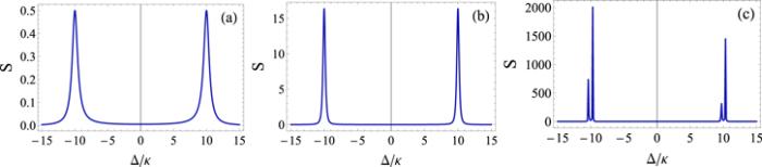
By considering a resonant interaction, such that Δ_a =Δ_b = Δ, in figure 1 we plot the intensity power spectrum as a function of the detuning Δ/κ in the strong coupling regime. This regime is reached when the exciton–photon constant coupling is much higher than the dissipation rates (g ≫ κ, γ). Before we introduce the nonlinear crystal (λ = 0), the spectrum shows two symmetrical resonant peaks around particular detunings given by Δ = ± g, i.e. separated by 2g, corresponding to the Rabi frequencies (figure 1(a)). When the amplitude of the squeezed drive λ reaches 0.8κ, we first observe that the whole system gains significantly in photonic intensity; then, a narrowing of the resonant peaks is achieved (figure 1(b)). For stronger squeezed pumping, λ = 1.2κ, the narrowing of the widths is much more visible. Additionally, the peaks are duplicated and the spectrum is no longer symmetrical (figure 1(c)). The number of peaks appearing in the spectrum can be explained on the basis of the eigenvalues of the system corresponding to equations (4) and (5). When the squeezed source does not act on the cavity, these eigenvalues can be approximated in the strong coupling regime as follows:(19)$\begin{eqnarray}{\beta }_{\mathrm{1,2}}\approx -\displaystyle \frac{1}{4}\left(\gamma +\kappa \right)+{\rm{i}}\left({\rm{\Delta }}\pm g\right).\end{eqnarray}$

Figure 1.

New window|Download| PPT slide
Figure 1.Transmitted field intensity plotted as a function of Δ/κ for γ = κ, ω − ω₀ = 0, n = 0.5, and g = 10κ. (a) λ = 0. (b) λ = 0.8κ. (c) λ = 1.2κ.


The real and imaginary parts of the eigenvalues determine the widths and positions of the peaks. The imaginary parts of β_1,2 indicate the position of the two peaks of figure 1(a) at around ±g. When the nonlinear material comes into play, λ ≠ 0, equations (4) and (5) have two additional eigenvalues given by ${\beta }_{3}\approx -(\tfrac{\gamma }{2}+{\rm{i}}{\rm{\Delta }})$ and ${\beta }_{4}\approx -(\tfrac{\kappa }{2}+{\rm{i}}{\rm{\Delta }})$, which explains the four resonant peaks of the intermixed photonic and excitonic states of figure 1(c).

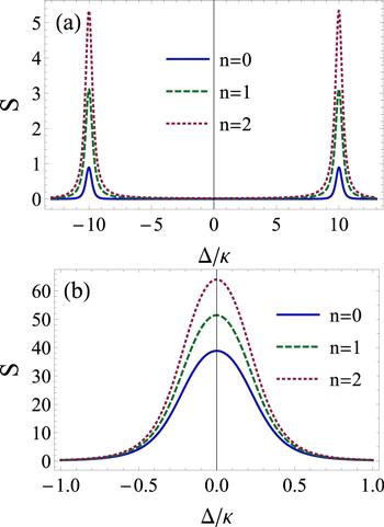
The effect of the temperature on the intensity spectrum of the transmitted field is illustrated by figure 2. For this, we fix the squeezed light amplitude at λ = 0.5κ and vary the thermal exciton mean number n = 0, 1, 2. We clearly observe that thermal excitations increase the transmitted intensity in the strong coupling regime (figure 2(a)) as well as in the weak coupling regime (figure 2(b)). For strong coupling, the temperature affects only the Rabi frequencies; the rest of the spectrum remains unchanged. For weak interactions, the maximal intensity is localized around the total resonance.

Figure 2.

New window|Download| PPT slide
Figure 2.Intensity spectrum of the transmitted field versus the frequency detuning Δ/κ for different values of the thermal exciton mean number n. (a) The strong coupling regime (g = 10κ). (b) The weak coupling regime (g = 0.2κ). The other parameters are chosen as follows: γ = κ, ω − ω₀ = 0, and λ = 0.5κ.


It is important to mention here that the small fluctuation approximation is applied around the steady-state value. It is therefore important to discuss the stability of the system. Stability means that when the operators of the system deviate from their corresponding mean values, they will return to these mean values if the fluctuation terms are dropped [24]. This kind of system is described by a non-Hermitian Hamiltonian H with complex eigenvalues ${{ \mathcal E }}_{k}={E}_{k}+\tfrac{{\rm{i}}}{2}{{\rm{\Gamma }}}_{k}$. These eigenvalues provide the energies E_k of the states and their lifetimes defined by the inverse of the widths Γ_k. The set of equations (4)–(5) has the form dU/dt = LU + F. If the matrix L has all eigenvalues such that the real part of each eigenvalue is negative, then the stability of the system is assured. From the expressions of the eigenvalues β_i given above, all their real parts are negative, so the system is stable.

4. Noise spectrum: light squeezing induced by the second-order nonlinearity

In this section, we examine the squeezing of the transmitted radiation. We also discuss the dependence of the nonclassical effect on the system parameters and show how the choice of suitable parameters is crucial in order to observe optimum squeezing. This can be investigated by introducing the noise spectrum of the output field, which can be measured by photodetectors and a frequency spectrum analyzer connected to them. It is defined as [33]:(20)$\begin{eqnarray}\begin{array}{rcl}{S}_{\theta }(\omega ) & = & {\displaystyle \int }_{-\infty }^{+\infty }\langle \delta {X}_{\theta }^{\mathrm{out}}(t+\tau )\delta {X}_{\theta }^{\mathrm{out}}(t){\rangle }_{{ss}}{{\rm{e}}}^{-{\rm{i}}(\omega -{\omega }_{0})\tau }{\rm{d}}\tau \\ & = & \langle \delta {X}_{\theta }^{\mathrm{out}}(\omega )\delta {X}_{\theta }^{\mathrm{out}}(\omega )\rangle ,\end{array}\end{eqnarray}$where ${X}_{\theta }^{\mathrm{out}}(\omega )={{\rm{e}}}^{-{\rm{i}}\theta }\delta {a}^{\mathrm{out}}(\omega )+{{\rm{e}}}^{{\rm{i}}\theta }\delta {a}^{\dagger \mathrm{out}}(\omega )$ is a field quadrature and θ designates its controllable phase. Equation (20) can then be rewritten as ${S}_{\theta }(\omega )={C}_{{aa}}^{\mathrm{out}}(\omega ){{\rm{e}}}^{-2{\rm{i}}\theta }\,+{C}_{{a}^{\dagger }{a}^{\dagger }}^{\mathrm{out}}(\omega ){{\rm{e}}}^{2{\rm{i}}\theta }+{C}_{{{aa}}^{\dagger }}^{\mathrm{out}}(\omega )+{C}_{{a}^{\dagger }a}^{\mathrm{out}}(\omega )$, where the correlation function ${C}_{{aa}}^{\mathrm{out}}(\omega )$ is given by $2\pi {C}_{{aa}}^{\mathrm{out}}(\omega )\delta (\omega +\omega ^{\prime} )\,=\langle \delta {a}^{\mathrm{out}}(\omega )\delta {a}^{\mathrm{out}}(\omega ^{\prime} )\rangle $. As we are interested in the optimal values of the nonclassical effect, we need to optimize the squeezing spectrum with respect to the phase angle θ by solving dS_θ(ω)/dθ = 0. The optimal angle θ_opt then satisfies ${{\rm{e}}}^{2{\rm{i}}{\theta }_{\mathrm{opt}}}=-{C}_{{aa}}^{\mathrm{out}}(\omega )/| {C}_{{aa}}^{\mathrm{out}}(\omega )| $. As a result, the optimized squeezing spectrum reads as follows: ${S}_{\mathrm{opt}}(\omega )\,=1+2[{C}_{{a}^{\dagger }a}^{\mathrm{out}}(\omega )-| {C}_{{aa}}^{\mathrm{out}}(\omega )| ]$. With the help of the standard input–output relations given earlier, and after some manipulations, we obtain ${C}_{{aa}}^{\mathrm{out}}(\omega )=\kappa ({C}_{{aa}}(\omega )-{{ \mathcal I }}_{3}(-\omega ))$, where the intracavity covariance function C_aa(ω) is given by:(21)$\begin{eqnarray}\begin{array}{rcl}{C}_{{aa}}(\omega ) & = & \kappa {{ \mathcal I }}_{1}(\omega ){{ \mathcal I }}_{3}(-\omega )+\gamma (n+1){{ \mathcal I }}_{2}(\omega ){{ \mathcal I }}_{4}(-\omega )\\ & & +\gamma n{{ \mathcal I }}_{4}(\omega ){{ \mathcal I }}_{2}(-\omega ).\end{array}\end{eqnarray}$

The other correlation function, ${C}_{{a}^{\dagger }a}^{\mathrm{out}}(\omega )$, is calculated in section 3. Finally, we obtain the following analytical relation for the outside optimum noise spectrum:(22)$\begin{eqnarray}\begin{array}{rcl}{S}_{\mathrm{opt}}(\omega ) & = & 1+2\kappa (\kappa | {{ \mathcal I }}_{3}(-\omega ){| }^{2}\\ & & +\gamma n| {{ \mathcal I }}_{2}(-\omega ){| }^{2}+\gamma (n+1)\\ & & \times | {{ \mathcal I }}_{4}(-\omega ){| }^{2})-2\kappa | (\kappa {{ \mathcal I }}_{1}(\omega ){{ \mathcal I }}_{3}(-\omega )\\ & & +\gamma (n+1)\times {{ \mathcal I }}_{2}(\omega ){{ \mathcal I }}_{4}(-\omega )\\ & & +\gamma n{{ \mathcal I }}_{4}(\omega ){{ \mathcal I }}_{2}(-\omega )-{{ \mathcal I }}_{3}(-\omega ))| .\end{array}\end{eqnarray}$

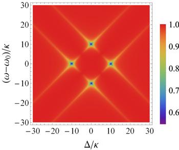
In figure 3, we show S_opt as a function of the detuning Δ/κ and the frequency (ω − ω₀)/κ in the strong coupling regime for λ = 0.5κ. The plot shows that the spectrum consists of four symmetrical resonant peaks corresponding to emitted squeezed photons on the output side of the cavity. This can be identified by the values of S_opt that are lower than unity. Away from these particular resonances, the light is coherent (S_opt = 1). Interestingly, we observe that maximal squeezing is realized either at a zero frequency for the Δ/κ ± g points, or at zero detuning for ω − ω₀ = ±g. The magnitude of squeezing in these peaks approaches 45%. This particular symmetry could be very useful for experimental investigations and helps to easily identify the maximal squeezing.

Figure 3.

New window|Download| PPT slide
Figure 3.Density plot of the squeezing spectrum versus the frequency (ω − ω₀)/κ and the frequency detuning Δ/κ in the strong coupling regime for γ = κ, λ = 0.5κ, n = 0, and g = 10κ.


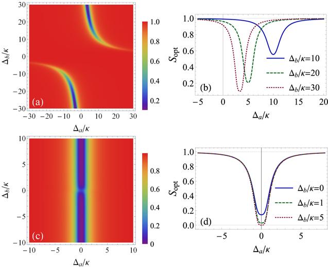
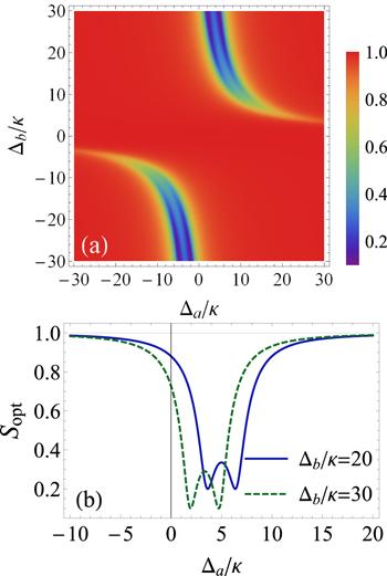
In a more generalized picture, we now consider different detunings. The variation of S_opt against Δ_a/κ and Δ_b/κ at a temperature of zero is depicted in figure 4, which shows two branches of squeezed light for strong exciton–photon coupling. Here, the amount of the nonclassical effect is more than 80%. An interesting behavior we observed is that the larger the pump–exciton detuning Δ_b, the higher the squeezing value. This means that to increase the degree of squeezing, we should tune the frequency of the coherent drive to be far from the excitonic mode frequency (figure 4(b)). Another important discovery concerns the fact that squeezing cannot occur when the coherent pumping is resonant with the excitonic mode (Δ_b = 0). Indeed, nonresonant excitation with respect to Δ_b appears to be a necessary condition for the emergence of the nonclassical effect in this system. For weak light–matter interactions, g≪κ, γ, the dynamical behavior of the system changes. The noise spectrum now exhibits a single branch of squeezed light around the pump–cavity resonance (Δ_a = 0) (figure 4(c)). In contrast to the case of strong coupling, the squeezing is very slightly dependent on the pump–exciton detuning, Δ_b. This is better illustrated by figure 4(d), where perfect squeezing is possible with an appropriate choice of the system parameters.

Figure 4.

New window|Download| PPT slide
Figure 4.Plots of the squeezing spectrum versus the frequency detunings. (a) and (b) The strong coupling regime (g = 10κ). (c) and (d) The weak coupling regime (g = 0.2κ). The other parameters are chosen to be γ = κ, λ = 0.5κ, ω − ω₀ = 0, and n = 0.


We now turn our attention to the effect of thermal excitations on the squeezed radiation. To this end, we fix the squeeze amplitude at λ = 0.5κ and elevate the temperature from n = 0 to n = 1 as depicted in figure 5(a). We first observe that the amount of squeezing is reduced from 35% to 15% for n = 0.3. Then, for n = 1 the squeezing vanishes completely and some fluctuations appear above the shot noise level (S_opt > 1). The excess of noise appears at the Rabi frequency. Obviously, a further increase of the thermal exciton mean number will lead to higher values of S_opt. While the squeezing totally disappears in some regions, it is resistant to this effect near the pump–cavity resonance and for high values of Δ_b (figure 5(b)). In conclusion, the temperature has a negative effect on the stability of the nonclassical light, and the degree of squeezing strongly relies on the thermal bath temperature.

Figure 5.

New window|Download| PPT slide
Figure 5.The squeezing spectrum plotted versus the frequency detunings. (a) S_opt as a function of Δ_a/κ for Δ_b = 10κ and some values of the thermal exciton mean number. (b) Density plot of S_opt as a function of Δ_a/κ and Δ_b/κ for n = 1.5. The other parameters are set to γ = κ, λ = 0.5κ, and g = 10κ. Even though the temperature elevation tends to destroy the squeezing, there are two frequency zones that exhibit higher resistance to this effect than the others.


Figure 6 illustrates the variation of the optimum squeezing spectrum versus the detunings for the stronger squeezed light amplitude given by λ = 1.5κ. As can be seen from this figure, the branches of squeezing outlined earlier become wider. This widening is accompanied by a duplication, and the two resulting branches correspond to optimal squeezing. This feature is further identified in figure 6(b), in which, for fixed Δ_b/κ, the duplicated peaks show the same amount of squeezing. Again, the choice of a large detuning, Δ_b, improves the nonclassical effect (dashed line).

Figure 6.

New window|Download| PPT slide
Figure 6.Plots of the squeezing spectrum versus frequency detunings in the strong coupling regime for γ = κ, λ = 1.5κ, ω − ω₀ = 0, n = 0, and g = 10κ.


As shown above, the system under consideration is able to generate large amount of squeezing. This light property is very useful for precise measurements. According to Heisenberg's uncertainty principle, the precision of any physical-quantity measurement is limited by quantum fluctuations appearing in the field which lead to the standard quantum limit. This quantum limit can be overcome using squeezed light, thus enhancing the measurement accuracy. Squeezed light is a typical nonclassical light, which shows reduced noise in one field quadrature component [34]. Furthermore, quantum noise reduction to levels lower than the shot-noise level is also used to avoid the loss of encoded information during quantum computation, leading to an accumulation of errors. Indeed, to reduce information loss, scientists have been experimenting with squeezing light by removing tiny quantum-level fluctuations. Kosuke Fukui et al [13] developed an approach that involves squeezing light by removing error-prone quantum bits when quantum bits cluster together.

5. Correlation function and the nature of the produced light

The second-order correlation function measures the degree of coherence between two fields. It is defined as the intensity–intensity correlation. In quantum mechanics, the autocorrelation function of the cavity field is defined as [35]:(23)$\begin{eqnarray}{g}^{(2)}(t,t+\tau )=\displaystyle \frac{\langle {a}^{\dagger }(t){a}^{\dagger }(t+\tau )a(t+\tau )a(t)\rangle }{\langle {a}^{\dagger }a{\rangle }^{2}}.\end{eqnarray}$

In the stationary regime, the previous function only depends on the time delay τ, thus g⁽²⁾(t, t + τ) ≡ g⁽²⁾(τ) = l⁽²⁾(τ)/l⁽²⁾( ∞ ). The cavity field operator is split into the sum of an average value ⟨a(t)⟩ and a fluctuation operator δ a(t), where ⟨δa(t)⟩ = 0. For a Gaussian distribution field, the correlation of the fluctuations of any three operators o₁, o₂, and o₃ of the field is zero: ⟨δo₁δo₂δo₃⟩ = 0. Additionally, the correlation of the fluctuations of four operators o₁, o₂, o₃, and o₄ is reduced to [35–37]:(24)$\begin{eqnarray}\begin{array}{rcl}\langle \delta {o}_{1}\delta {o}_{2}\delta {o}_{3}\delta {o}_{4}\rangle & = & \langle \delta {o}_{1}\delta {o}_{2}\rangle \langle \delta {o}_{3}\delta {o}_{4}\rangle \\ & & +\langle \delta {o}_{1}\delta {o}_{3}\rangle \langle \delta {o}_{2}\delta {o}_{4}\rangle \\ & & +\langle \delta {o}_{1}\delta {o}_{4}\rangle \langle \delta {o}_{2}\delta {o}_{3}\rangle .\end{array}\end{eqnarray}$

The Gaussian approximation assumes that the field distribution is slightly modified compared to a Gaussian distribution. The two last relations are therefore valid. In this limit, the l⁽²⁾(τ) function can be expressed as:(25)$\begin{eqnarray}\begin{array}{rcl}{l}^{(2)}(\tau ) & = & {k}_{1}(\tau )+{k}_{2}(\tau )+{k}_{3}(\tau )\\ & & +{k}_{4}(\tau )+\langle {a}^{\dagger }{\rangle }^{2}\langle a{\rangle }^{2},\end{array}\end{eqnarray}$with:(26)$\begin{eqnarray}{k}_{1}(\tau )=2\mathrm{Re}\{{C}_{{a}^{\dagger }a}(\tau )\}\langle {a}^{\dagger }\rangle \langle a\rangle ,\end{eqnarray}$(27)$\begin{eqnarray}{k}_{2}(\tau )=2\mathrm{Re}\{{C}_{{aa}}(\tau )\langle {a}^{\dagger }{\rangle }^{2}\},\end{eqnarray}$(28)$\begin{eqnarray}{k}_{3}(\tau )=\{\langle \delta {a}^{\dagger }(\tau )\delta a(\tau )\rangle +\langle \delta {a}^{\dagger }(0)\delta a(0)\rangle \}\langle {a}^{\dagger }\rangle \langle a\rangle ,\end{eqnarray}$(29)$\begin{eqnarray}\begin{array}{rcl}{k}_{4}(\tau ) & = & {\left({C}_{{aa}}(\tau )\right)}^{* }{C}_{{aa}}(\tau )+{\left({C}_{{a}^{\dagger }a}(\tau )\right)}^{* }{C}_{{a}^{\dagger }a}(\tau )\\ & & +{\left({C}_{{a}^{\dagger }a}(0)\right)}^{* }{C}_{{a}^{\dagger }a}(0).\end{array}\end{eqnarray}$

The fluctuations in the cavity field are assumed to be very weak compared to the mean values, so that the inequality ⟨δa^†(τ)δa(0)⟩ ≪ ⟨a^†⟩⟨a⟩ is fulfilled. As a consequence, we can neglect the k₄ function, as it contains fourth-order fluctuation quantities. Additionally, it is possible to show in a straightforward manner that k₃(τ) + ⟨a^†⟩²⟨a⟩² ≃ ⟨a^†a⟩². We then obtain a simple linearized expression of the autocorrelation function:(30)$\begin{eqnarray}{g}^{(2)}(\tau )\simeq 1+\displaystyle \frac{{k}_{1}(\tau )+{k}_{2}(\tau )}{{\left(\langle a\rangle \langle {a}^{\dagger }\rangle \right)}^{2}},\end{eqnarray}$

I_a = ⟨a⟩⟨a^†⟩ is the steady-state photonic intensity. In order to simplify the calculation, we use a bilateral Laplace transformation by setting p = iω. This allows us to obtain more manageable expressions than those of the Fourier transformation. The evolution equations of the fluctuations are now:(31)$\begin{eqnarray}M(p)\left(\begin{array}{c}\delta a(p)\\ \delta b(p)\\ \delta {a}^{\dagger }(p)\\ \delta {b}^{\dagger }(p)\end{array}\right)=\left(\begin{array}{c}\sqrt{\kappa }{a}^{\mathrm{in}}(p)\\ \sqrt{\gamma }{b}^{\mathrm{in}}(p)\\ \sqrt{\kappa }{a}^{\mathrm{in}\dagger }(p)\\ \sqrt{\gamma }{b}^{\mathrm{in}\dagger }(p)\end{array}\right).\end{eqnarray}$

The evolution matrix M(p) is expressed in Laplace space as follows:(32)$\begin{eqnarray}M(p)=\left(\begin{array}{cccc}{\beta }_{1-} & -g & -\lambda & 0\\ g & {\beta }_{2-} & 0 & 0\\ -\lambda & 0 & {\beta }_{1+} & -g\\ 0 & 0 & g & {\beta }_{2+}\end{array}\right),\end{eqnarray}$with ${\beta }_{1\mp }(p)=p\mp {\rm{i}}{{\rm{\Delta }}}_{a}+\tfrac{\kappa }{2}$ and ${\beta }_{2\mp }(p)=p\mp {\rm{i}}{{\rm{\Delta }}}_{b}+\tfrac{\gamma }{2}$.

The solution of equation (31) for δa(p) is a linear combination of the incoming fluctuations that can be expressed in a general form as follows:(33)$\begin{eqnarray}\begin{array}{rcl}\delta a(p) & = & \sqrt{\kappa }{{ \mathcal I }}_{1}(p){a}^{\mathrm{in}}(p)+\sqrt{\gamma }{{ \mathcal I }}_{2}(p){b}^{\mathrm{in}}(p)\\ & & +\sqrt{\kappa }{{ \mathcal I }}_{3}(p){a}^{\mathrm{in}\dagger }(p)+\sqrt{\gamma }{{ \mathcal I }}_{4}(p){b}^{\mathrm{in}\dagger }(p).\end{array}\end{eqnarray}$

The intracavity covariances C_aa (p) and ${C}_{{a}^{\dagger }a}(p)$ are written as:(34)$\begin{eqnarray}\begin{array}{rcl}{C}_{{aa}}(p) & = & \kappa {{ \mathcal I }}_{1}(p){{ \mathcal I }}_{3}(-p)+\gamma (n+1){{ \mathcal I }}_{2}(p){I}_{4}(-p)\\ & & +\gamma n{{ \mathcal I }}_{4}(p){{ \mathcal I }}_{2}(-p),\end{array}\end{eqnarray}$(35)$\begin{eqnarray}\begin{array}{rcl}{C}_{{a}^{\dagger }a}(p) & = & \kappa {{ \mathcal I }}_{3}^{* }(p){{ \mathcal I }}_{3}(-p)+\gamma n{{ \mathcal I }}_{2}^{* }(p){{ \mathcal I }}_{2}(-p)\\ & & +\gamma (n+1){{ \mathcal I }}_{4}^{* }(p){{ \mathcal I }}_{4}(-p).\end{array}\end{eqnarray}$

The Laplace transform of the real part of a given function in τ gives the real part of the function in the variable p. Based on this property, the correlation function is given by:(36)$\begin{eqnarray}{g}^{(2)}(p)=1+\displaystyle \frac{2\mathrm{Re}\{{I}_{a}{C}_{{a}^{\dagger }a}(p)+\langle {a}^{\dagger }{\rangle }^{2}{C}_{{aa}}(p)\}}{{I}_{a}^{2}}.\end{eqnarray}$

We now decompose the ${{ \mathcal I }}_{i}(p)$ functions into a ratio of two polynomials in p as ${{ \mathcal I }}_{i=\mathrm{1,2},\mathrm{3,4}}(p)={\zeta }_{i=1,2,3,4}^{{\prime} }(p)/\zeta (p)$, where $\zeta (p)=\det (M(p))$. Then, g⁽²⁾(p) becomes:(37)$\begin{eqnarray}\begin{array}{rcl}{g}^{(2)}(p) & = & 1+\displaystyle \frac{2}{{I}_{a}{\zeta }^{* }(p)\zeta (-p)}\mathrm{Re}[\kappa {\zeta }_{3}^{{\prime} * }(p){\zeta }_{3}^{{\prime} }(-p)\\ & & \,+\gamma n{\zeta }_{2}^{{\prime} * }(p){\zeta }_{2}^{{\prime} }(-p)+\gamma (n+1){\zeta }_{4}^{{\prime} * }(p){\zeta }_{4}^{{\prime} }(-p)]\\ & & \,+\displaystyle \frac{2}{{I}_{a}^{2}\zeta (p)\zeta (-p)}\mathrm{Re}[\langle {a}^{\dagger }{\rangle }^{2}(\kappa {\zeta }_{1}^{{\prime} }(p){\zeta }_{3}^{{\prime} }(-p)\\ & & \,+\gamma (n+1){\zeta }_{2}^{{\prime} }(p){\zeta }_{4}^{{\prime} }(-p)+\gamma n{\zeta }_{4}^{{\prime} }(p){\zeta }_{2}^{{\prime} }(-p))].\end{array}\end{eqnarray}$

The final step consists of the determination of the inverse Laplace transform of the previous function. For this, we first calculate the poles of g⁽²⁾(p). After that, we use the symmetry property of the autocorrelation function, which means that only poles with negative real parts are considered.

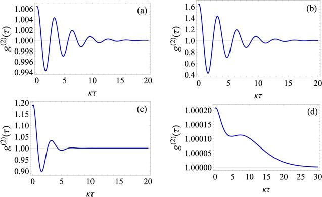
The second-order correlation function of the transmitted light is depicted as a function of the normalized time in figure 7. We observe that in the strong coupling regime, it is a damped oscillatory function. After long delays g⁽²⁾(τ) → 1. For strong pumping, ϵ = 100κ, the oscillation amplitudes of g⁽²⁾(τ) are very weak. The cavity photon field statistics approach coherent statistics (figure 7(a)). By reducing the pumping to ϵ = 5κ, the oscillation amplitudes increase. At the initial moment, the value of g⁽²⁾(0) is greater than unity, indicating a super-Poissonian behavior leading to a classical bunching effect (figure 7(b)). The photons tend to leave the cavity through the end mirror in groups. To see the effect of more strongly squeezed light, we increase λ to 2κ. Consequently, the number of oscillations decreases and the function is rapidly damped toward the stationary regime for relatively short delays (figure 7(c)). Moreover, the magnitude of the bunching effect is reduced. It should be noted that in the strong-driving limit, the second-order nonlinearity is unable to generate antibunched light as was observed with third-order nonlinearities. Furthermore, for a linear system, the cavity transforms the incoming coherent state to another coherent state (g⁽²⁾(τ) = 1). In the case of weak light–matter coupling (g = κ/10), the oscillatory behavior of the function vanishes and the emitted radiation is coherent (figure 7(d)). We note here that a dipolariton cavity interacting with an OPO exhibits a similar behavior and generates the same type of light [30].

Figure 7.

New window|Download| PPT slide
Figure 7.The second-order correlation function of photons g⁽²⁾(τ) versus normalized time κτ. (a) ϵ = 100κ, λ = κ, and g = 20κ. (b) ϵ = 5κ, λ = κ, and g = 20κ. (c) ϵ = 5κ, λ = 2κ, and g = 20κ. (d) ϵ = 5κ, λ = 0.7κ, and g = κ/10. For all plots, the other parameters are γ = κ, Δ = 0.3κ, and n = 1.


Finally, we note that when the exciton–exciton interaction is non-negligible, the intensity and noise spectra become excitonic intensity dependant. It has been demonstrated that in the absence of exciton–exciton interactions, the exciton has no resonance fluorescence. The exciton–exciton interaction switches on resonance fluorescence, and the fluorescence spectrum is split into two peaks when the pumping field exceeds a critical value [24]. The excitonic nonlinearity may lead also to nonclassical statistical properties, and the emitted light is antibunched [4].

6. Conclusions

We studied a system consisting of an optical cavity that includes a quantum well interacting with a second-order nonlinear crystal. We have shown that the intensity spectrum is formed of two peaks centered around particular frequency detunings. The application of the squeezed source strongly affects the spectrum by causing narrowing and duplication of the resonant peaks. The noise spectrum exhibits two branches of squeezed light. Importantly, an increase of the pump–exciton detuning strongly enhances the degree of squeezing. We have also shown that the weak coupling regime is favorable to perfectly squeezed radiation. Despite the fact that interactions with the thermal environment tend to destroy the nonclassical effect, there are particular frequency detunings that permit us to observe high resistance to increasing temperatures.

For weak coherent pumping, the second-order correlation function is a damped oscillatory function. It shows super-Poissonian statistics leading to bunched light. An increase in the squeezed light amplitude reduces the oscillations of the function and the magnitude of the bunching. The oscillatory behavior completely vanishes in the weak coupling regime and the transmitted light becomes almost coherent.

Reference View Option By original order
By published year
By cited within times
By Impact factor

[1]Kavokin A Malpuech G 2003 Cavity Polaritons Amsterdam Elsevier
[Cited within: 1]

[2]Vahala K 2004 Optical Microcavities Singapore World Scientific Publishing
[Cited within: 1]

[3]Press D Gotzinger S Reitzenstein S Hofmann C Loffler A Kamp M Forchel A Yamamoto Y 2007 Phys. Rev. Lett. 98 117402
DOI:10.1103/PhysRevLett.98.117402 [Cited within: 1]

[4]Eleuch H Courty J M Messin G Fabre C Giacobino E 1999 J. Opt. B: Quantum Semiclass 1 1
DOI:10.1088/1464-4266/1/1/001 [Cited within: 3]

[5]Safavi-Naeini A H Mayer Alegre T P Chan J Eichenfield M Winger M Lin Q Hill J T Chang D E Painter O 2011 Nature 472 69
DOI:10.1038/nature09933 [Cited within: 1]

[6]Pikovski I Vanner M R Aspelmeyer M Kim M S Brukner C 2011 Nature Phys. 8 393
DOI:10.1038/nphys2262 [Cited within: 1]

[7]Hillery M 2000 Phys. Rev. A 61 022309
DOI:10.1103/PhysRevA.61.022309 [Cited within: 1]

[8]Gottesman D Preskill J 2001 Phys. Rev. A 63 022309
DOI:10.1103/PhysRevA.63.022309

[9]Gisin N Ribordy G Tittel W Zbinden H 2002 Rev. Mod. Phys. 74 145
DOI:10.1103/RevModPhys.74.145 [Cited within: 1]

[10]Eberle T Steinlechner S Bauchrowitz J Handchen V Vahlbruch H Mehmet M Muller-Ebhardt H Schnabel R 2010 Phys. Rev. Lett. 104 251102
DOI:10.1103/PhysRevLett.104.251102 [Cited within: 1]

[11]LIGO Scientific Collaboration 2011 A gravitational wave observatory operating beyond the quantum shot-noise limit
Nat. Phys. 7 962 965
DOI:10.1038/nphys2083 [Cited within: 1]

[12]Menicucci N C van Loock P Gu M Weedbrook C Ralph T C Nielsen M A 2006 Phys. Rev. Lett. 97 110501
DOI:10.1103/PhysRevLett.97.110501 [Cited within: 1]

[13]Fukui K Tomita A Okamoto A 2018 Phys. Rev. X 8 021054
[Cited within: 1]

[14]O'Brien J L 2007 Science 318 1567 1570
DOI:10.1126/science.1142892

[15]Menicucci N C Flammia S T Pfister O 2008 Phys. Rev. Lett. 101 130501
DOI:10.1103/PhysRevLett.101.130501 [Cited within: 1]

[16]Bergman K Doerr C R Haus H A Shirasaki M 1993 Opt. Lett. 18 643 645
DOI:10.1364/OL.18.000643 [Cited within: 1]

[17]Kolobov M I Kumar P 1993 Opt. Lett. 18 849 851
DOI:10.1364/OL.18.000849

[18]Wang S Xiang X Treps N Fabre C Liu T Zhang S Dong R 2018 Phys. Rev. A 98 053821
DOI:10.1103/PhysRevA.98.053821 [Cited within: 1]

[19]Hoff U B Harris G I Madsen L S Kerdoncuff H Lassen M Nielsen B M Bowen W P Andersen U L 2013 Opt. Lett. 38 1413 1415
DOI:10.1364/OL.38.001413 [Cited within: 1]

[20]Yamamoto Y Tassone F Cao H 2000 Semiconductor Cavity Quantum Electrodynamics Berlin Springer
[Cited within: 1]

[21]Miller R Northup T E Birnbaum K M Boca A Boozer A D Kimble H J 2005 J. Phys. B: At. Mol. Opt. Phys. 38 S551
DOI:10.1088/0953-4075/38/9/007

[22]Jabri H Eleuch H 2011 Comm. Theor. Phys. 56 134 138
DOI:10.1088/0253-6102/56/1/23 [Cited within: 1]

[23]Cao C-Q Cao H Liu Y-X 2000 Phys. Rev. B 62 16453
DOI:10.1103/PhysRevB.62.16453 [Cited within: 1]

[24]Liu Y-X Cao C-Q Cao H 2000 Phys. Rev. A 61 023802
DOI:10.1103/PhysRevA.61.023802 [Cited within: 3]

[25]Jabri H Eleuch H 2020 Phys. Rev. A 102 063713
DOI:10.1103/PhysRevA.102.063713 [Cited within: 1]

[26]Jabri H Eleuch H 2018 J. Opt. Soc. Am. B 35 2317 2325
DOI:10.1364/JOSAB.35.002317

[27]Jabri H Eleuch H 2020 J. Opt. Soc. Am. B 37 A9
DOI:10.1364/JOSAB.393833

[28]Jabri H Eleuch H 2018 J. Opt. 20 055201
DOI:10.1088/2040-8986/aab753

[29]Jabri H Eleuch H 2019 Annalen Der Physik (Berlin) 531 1900253
DOI:10.1002/andp.201900253

[30]Jabri H Eleuch H 2020 Phys. Rev. A 101 053819
DOI:10.1103/PhysRevA.101.053819 [Cited within: 2]

[31]Collet M J Gardiner C W 1984 Phys. Rev. A 30 1386
DOI:10.1103/PhysRevA.30.1386 [Cited within: 1]

[32]Reynaud S Heidmann A 1989 Opt. Commun. 71 209
DOI:10.1016/0030-4018(89)90429-X [Cited within: 1]

[33]Helico L Fabre C Reynaud S Giacobino E 1992 Phys. Rev. A 46 4397
DOI:10.1103/PhysRevA.46.4397 [Cited within: 1]

[34]Heng-Xin S Kui L Jun-Xiang Z Jiang-Rui G 2015 Acta Phys. Sin. 64 234210
[Cited within: 1]

[35]Mandel L Wolf E 1995 Optical Coherence and Quantum Optics Cambridge Cambridge University Press
[Cited within: 2]

[36]Kampen N G Van 1981 Stochastic Processes in Physics and Chemistry North Holland Elsevier


[37]Gardiner C W 1983 Handbook of Stochastic Methods Berlin Springer
[Cited within: 1]