Yan Yu¹, Nan Zhao^,1, Chang-xing Pei¹, Wei Li²¹State Key Laboratory of Integrated Services Networks, Xidian University, Xi’an, 710071, China
²Cloud Computing Center of Xi’an branch of Shaanxi Telecom, China Telecom, Xi’an, 710002, China

Received:2021-02-4Revised:2021-04-19Accepted:2021-04-21Online:2021-07-02

Fund supported:

*Key Industry Projects in Shaanxi Province.2019ZDLGY09-03 Key Industry Projects in Shaanxi Province.2020ZDLGY15-09 National Natural Science Foundation of China.61771296 National Natural Science Foundation of China.61372076 National Natural Science Foundation of China.61301171 Natural Science Foundation of Shaanxi province.2018JM60-53 Natural Science Foundation of Shaanxi province.2018JZ60-06 111 Project under Grant.B08038

Abstract
Multicast-based quantum teleportation (QT) is extensively used in quantum information transmission where a sender sends different information to multiple receivers at the large distance through the quantum entangled channel. In this paper, we introduce the multi-output QT scheme, which deals with the situation that the synchronous transfer of the arbitrary m- and (m+1)-qubit GHZ-class states from one sender to two receivers. Notably, the requirement about synchronous diverse information transmission is satisfied in our scheme with high efficiency. Moreover, we demonstrate the implementation of the special case of above quantum multi-output teleportation scheme on a sixteen-qubit quantum computer and a 32-qubit simulator provided by IBM quantum platform, then discuss it in four types of noisy environments, and calculate the fidelities of the output states.
Keywords： quantum multicast communications;multi-output quantum teleportation;IBM quantum experience


PDF (555KB)MetadataMetricsRelated articlesExportEndNote|Ris|BibtexFavorite
Cite this article
Yan Yu, Nan Zhao, Chang-xing Pei, Wei Li. Multi-output quantum teleportation of different quantum information with an IBM quantum experience^*. Communications in Theoretical Physics, 2021, 73(8): 085103- doi:10.1088/1572-9494/abf9fe

1. Introduction

Quantum entanglement is a significant resource in quantum information and quantum computation. By employing entanglement, schemes for quantum teleportation (QT) drew considerable attention of the quantum communication community since its introduction in 1993 [1]. Four years later, Bouwmeester et al [2] first experimentally verified this theoretical scheme using pairs of polarization-entangled photons. Then different entanglement channels were utilized in various QT schemes, such as W state [3, 4], cluster state [5] and GHZ-like states [6, 7], etc.

As a natural generalization of QT, the multiparty protocols for the multi-qubit quantum information transmission have also been proposed [8–22] in recent years. In 2002, Bei et al [8] presented two kinds of teleportation protocols for the m-particle d-dimensional Schmidt-form entangled state. In 2011, a multiparty-controlled teleportation scheme was reported by Long et al [9] to teleport an arbitrary high-dimensional GHZ-class state. In recent years, Yu [10] gave a multi-output QT scheme of two arbitrary single-qubit states from one sender to two receivers, respectively and synchronously. In 2018, Choudhury [11] utilized a single entangled channel to teleport a two-qubit and two single-qubit quantum states synchronously. By the three-qubit non-maximally entangled states, Wei [12] introduced an efficient controlled teleportation of arbitrary multi-qubit state. In 2019, Li [13] designed a novel QT scheme of multiple arbitrary qubits, taking advantage of the properties of quantum walks. Zhou [14] realized the cyclic and bidirectional QT by taking the pseudo multi-qubit entangled state as the quantum channel. In 2020, by the seven-qubit entangled channel, a novel theoretical scheme was put forward to implement quantum cyclic controlled teleportation of three unknown states [15]. Yang et al [16] discussed the teleportation of particles in an environment of an N-body system.

However, due to the high cost of quantum resources, hardly any QT protocol of multi-qubit quantum state has been tested experimentally. Here, an interesting window-IBM Q Experience for experimental realization of the quantum computation and communication schemes has been opened up recently. It offers a cloud-based quantum computing platform, allowing the users to design quantum circuits and test those circuits, both on the real IBM quantum computer and the IBM simulators. Any user can create a quantum circuit on the five-qubit [23], fourteen-qubit [24], sixteen-qubit [25] and 53-qubit [26] computers for a real run or simulation, including quantum simulation [27, 28], developing quantum algorithms [29], testing of quantum information theoretical tasks [30], QT [31, 32], quantum applications [33] to name a few.

Although over the past few decades, the multi-party QT schemes of multi-qubit state are constantly presented and improved, the requirements about the multicast-mode QT of multi-qubit state and synchronous diverse information transmission are not satisfied. In order to solve these problems, we propose the QT scheme to synchronously teleport many arbitrary high-dimensional GHZ-class states from one sender to multiple receivers, and implement the special case of the proposed scheme with a sixteen-qubit quantum computer and a 32-qubit simulator on IBM quantum platform. To be specific, the sender Alice wants to transmit an m-qubit GHZ-class state to receiver Bob and an (m+1)-qubit GHZ-class state to receiver Charlie synchronously. In particular, we have successfully implemented the special case of the multi-output QT circuit to teleport the different information from one sender to two distant receivers. Besides, we discuss the impacts on the special case of the multi-output QT scheme via four types of noisy environments (amplitude-damping noise, phase-damping noise, bit-flip noise and phase-flip noise), and calculate the fidelities of the output states. It may show some light and pave the way for future realizations of the proposed multi-output QT schemes.

2. Multi-output QT of a single-qubit state and a two-qubit state

2.1. Theoretical description

In this protocol, sender Alice wants to teleport an arbitrary single-qubit state $| \chi {{\prime} }_{1}\rangle $ to receiver Bob, in the meanwhile, to teleport an arbitrary two-qubit state ∣χ″₂⟩ to receiver Charlie, respectively. In detail, the unknown states which are held by Alice can be expressed as(1)$\begin{eqnarray}| \chi {{\prime} }_{1}\rangle ={\left({\alpha }_{1}| 0\rangle +{\beta }_{1}| 1\rangle \right)}_{1},| \chi {{\prime\prime} }_{2}\rangle ={\left({\alpha }_{2}| 00\rangle +{\beta }_{2}| 11\rangle \right)}_{23},\end{eqnarray}$where the parameters α_i, β_i satisfy the normalized condition ∣α_i∣² + ∣β_i∣² = 1(i = 1, 2). Now, the detailed implementation of this protocol is shown as the follows.

(S₁) Suppose that three participants share a five-qubit entangled state shown as equation (2), ∣ψ⟩₁₂₃₄₅, with Alice keeping the particles (1, 2), Bob holding the particle 3, and Charlie is in possession of the particles (4, 5),(2)$\begin{eqnarray}\begin{array}{l}| {\rm{\Psi }}{\rangle }_{12345}=\displaystyle \frac{1}{2}\left(| 00000\rangle +| 01011\rangle +| 10100\rangle \right.\\ {\left.+| 11111\rangle \right)}_{12345}.\end{array}\end{eqnarray}$Thus the state of composite system turns to(3)$\begin{eqnarray}\begin{array}{rcl}| {\rm{\Omega }}{\rangle }_{T} & = & | \chi {{\prime} }_{1}{\rangle }_{1}\otimes | \chi {{\prime\prime} }_{2}{\rangle }_{23}\otimes | {\rm{\Psi }}{\rangle }_{{A}_{1}{A}_{2}{{BC}}_{1}{C}_{2}}\\ & = & {\left({\alpha }_{1}| 0\rangle +{\beta }_{1}| 1\rangle \right)}_{1}\otimes {\left({\alpha }_{2}| 00\rangle +{\beta }_{2}| 11\rangle \right)}_{23}\\ & & \otimes \displaystyle \frac{1}{2}\left(| 00000\rangle +| 01011\rangle +| 10100\rangle \right.\\ & & {\left.+| 11111\rangle \right)}_{{A}_{1}{A}_{2}{{BC}}_{1}{C}_{2}}.\end{array}\end{eqnarray}$

(S₂) Alice firstly performs two Bell state measurements (BSMs) on her particles (1, A₁) and (2, A₂), respectively. Then she performs a Hadamard operation (H) on the remaining particle (3). Here, the BSM basis are expressed as follows,(4)$\begin{eqnarray}| {\phi }^{\pm }\rangle =\displaystyle \frac{1}{\sqrt{2}}(| 00\rangle \pm | 11\rangle ),| {\varphi }^{\pm }\rangle =\displaystyle \frac{1}{\sqrt{2}}(| 01\rangle \pm | 10\rangle ),\end{eqnarray}$and the Hadamard operation is $| \pm \rangle =\tfrac{1}{\sqrt{2}}(| 0\rangle \pm | 1\rangle )$.

Alice communicates her measurement outcomes to receivers via the classical channel, in the meanwhile, two receivers’ particles will collapse into the superposition $| \tau {\rangle }_{{{BC}}_{1}{C}_{2}}$.

(S₃) According to the above measurement outcomes, Bob and Charlie perform the recovery operations on their own particles. If Alice detects the particles in the states $| {\varphi }^{+}{\rangle }_{(1,{A}_{1})}$, $| {\varphi }^{+}{\rangle }_{(2,{A}_{2})}$ and ∣ + ⟩₃, the state of particles $| \tau {\rangle }_{{{BC}}_{1}{C}_{2}}$ will collapse into the product state:(5)$\begin{eqnarray}| \tau {\rangle }_{{{BC}}_{1}{C}_{2}}=\displaystyle \frac{1}{4\sqrt{2}}{\left({\alpha }_{1}| 1\rangle +{\beta }_{1}| 0\rangle \right)}_{B}\otimes {\left({\alpha }_{2}| 11\rangle +{\beta }_{2}| 00\rangle \right)}_{{C}_{1}{C}_{2}}.\end{eqnarray}$

As is shown in the equation (5) clearly, Bob performs unitary operation Σ_x on particle B, in the meanwhile, Charlie performs Σ_x ⨂ Σ_x on particle (C₁, C₂). These lead to the final states, ${\left({\alpha }_{1}| 0\rangle +{\beta }_{1}| 1\rangle \right)}_{B}$ and ${\left({\alpha }_{2}| 00\rangle +{\beta }_{2}| 11\rangle \right)}_{{C}_{1}{C}_{2}}$, which are the required output states of the multi-output QT scheme. Table 1 above shows sender’s measurement results (eg. $| {\varphi }^{+}{\rangle }_{(1,{A}_{1})}$) and the unitary operations performed by two receivers to recover the quantum states as equation (1).


Table 1.
Table 1.Measurement results and unitary operations of each party in proposed scheme taking $| {\varphi }^{+}{\rangle }_{(1,{A}_{1})}$ as an example.

Alice’s results			Bob’s operation	Charlie’s operation
$| {\varphi }^{+}{\rangle }_{(1,{A}_{1})}$	$| {\phi }^{+}{\rangle }_{(2,{A}_{2})}$	∣ + ⟩3	Σx	I ⨂ I
		∣ − ⟩3	Σx	Σz ⨂ I
	$| {\phi }^{-}{ \rangle }_{(2,{A}_{2})}$	∣ + ⟩3	Σx	Σz ⨂ I
		∣ − ⟩3	Σx	I ⨂ I
	$| {\varphi }^{+}{\rangle }_{(2,{A}_{2})}$	∣ + ⟩3	Σx	Σx ⨂ Σx
		∣ − ⟩3	Σx	Σx ⨂ iΣy
	$| {\varphi }^{-}{ \rangle }_{(2,{A}_{2})}$	∣ + ⟩3	Σx	Σx ⨂ iΣy
		∣ − ⟩3	Σx	Σx ⨂ Σx

New window|CSV

2.2. Implementation and results

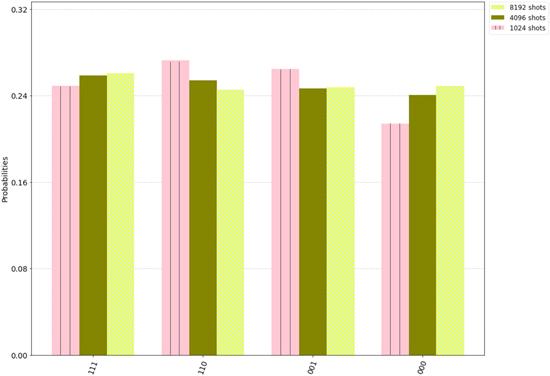
Based on the above discussion, by choosing different number of shots, the real experiment of the above-mentioned QT scheme has been executed using the quantum processor in IBM quantum experience interface. Here, shots denote the number of times the given experiment runs in a quantum processor. After running the experiment in the quantum processor for several times, the results will be displayed in the form of a histogram. In the histogram, each bar stands the probability of getting one of the possible results for the experiment. Figure 1 shows the results of the above-mentioned QT scheme by a 32-qubit simulator, and the corresponding bar diagrams for different sets of number of shots, respectively.

Figure 1.

New window|Download| PPT slide
Figure 1.The bar plot comparison of the results obtained from real device are colored yellow, olive and pink for shots 8192, 4096 and 1024, respectively.


After running with different sets of number of shots respectively, the results are shown in table 2. Compared with theoretical results, it is apparently that the statistical accuracy can be improved by increasing the number of shots. That is why we all use 8192 shots in the analysis below.


Table 2.
Table 2.Simulated results of multi-output teleportation scheme.

No. of shots	Probability	Probability	Probability	Probability
	of ∣000⟩	of ∣001⟩	of ∣110⟩	of ∣111⟩
1024	0.286	0.234	0.243	0.236
4096	0.266	0.246	0.238	0.250
8192	0.247	0.247	0.245	0.261
ideal	0.250	0.250	0.250	0.250

New window|CSV

In table 3, we have shown the data taken for 9 runs by a 32-qubit simulator, each run having 8192 shots. According to the average value and standard deviation, the average error between the experimental and theoretical results is 0.004.


Table 3.
Table 3.Results of multi-output teleportation scheme, and the number of shots used for each is 8192.

Runs	Probability	Probability	Probability	Probability
	of ∣000⟩	of ∣001⟩	of ∣110⟩	of ∣111⟩
1	0.240	0.264	0.251	0.245
2	0.244	0.258	0.254	0.244
3	0.241	0.251	0.256	0.252
4	0.244	0.259	0.255	0.242
5	0.249	0.255	0.249	0.247
6	0.243	0.246	0.258	0.253
7	0.251	0.249	0.254	0.246
8	0.253	0.255	0.247	0.245
9	0.249	0.252	0.248	0.251

New window|CSV

In table 4, we compare the results in a 32-qubit simulator and the IBM-16-Melbourne for the above states, which is caused by the decoherence effects, gate errors, state preparation error and other factors.


Table 4.
Table 4.Results of IBM qasm simulator and IBM-16-Melbourne.

Probability	32-qubit	IBM-16—
of states	simulator	Melbourne
∣000⟩	0.240	0.142
∣001⟩	0.264	0.134
∣010⟩	0	0.139
∣011⟩	0	0.120
∣100⟩	0	0.124
∣101⟩	0	0.122
∣110⟩	0.251	0.117
∣111⟩	0.245	0.102

New window|CSV

2.3. Effects of the noisy environments

In this section, we will discuss the effects of traveling particles in the above-mentioned scheme, when they pass through the four noisy environments, including amplitude-damping (E_A), phase-damping noise (E_P), bit-flip noise (E_B), and phase-flip noise (E_W). These noise models are characterized by Kraus operators [34] given as follows,(6)$\begin{eqnarray}\begin{array}{rcl}(a){E}_{0}^{A} & = & \left[\begin{array}{cc}1 & 0\\ 0 & \sqrt{1-{\eta }_{A}}\end{array}\right],\,{E}_{1}^{A}=\sqrt{{\eta }_{A}}\left[\begin{array}{cc}0 & 1\\ 0 & 0\end{array}\right],\\ (b){E}_{0}^{P} & = & \sqrt{1-{\eta }_{P}}\left[\begin{array}{cc}1 & 0\\ 0 & 1\end{array}\right],\,{E}_{1}^{P}=\sqrt{{\eta }_{P}}\left[\begin{array}{cc}1 & 0\\ 0 & 0\end{array}\right],\\ {E}_{2}^{P} & = & \sqrt{{\eta }_{P}}\left[\begin{array}{cc}0 & 0\\ 0 & 1\end{array}\right],\\ (c){E}_{0}^{B} & = & \sqrt{1-{\eta }_{B}}\left[\begin{array}{cc}1 & 0\\ 0 & 1\end{array}\right],\,{E}_{1}^{B}=\sqrt{{\eta }_{B}}\left[\begin{array}{cc}0 & 1\\ 1 & 0\end{array}\right],\\ (d){E}_{0}^{W} & = & \sqrt{1-{\eta }_{W}}\left[\begin{array}{cc}1 & 0\\ 0 & 1\end{array}\right],\,{E}_{1}^{W}=\sqrt{{\eta }_{W}}\left[\begin{array}{cc}1 & 0\\ 0 & -1\end{array}\right],\end{array}\end{eqnarray}$where η_i(η_i ∈ [0, 1])(i = A, P, B, W) denote the error probabilities of traveling particles passing through four noisy environments. We suppose that the sender Alice prepares the shared state$| {\rm{\Psi }}{\rangle }_{{A}_{1}{A}_{2}{{BC}}_{1}{C}_{2}}$ in her laboratory, and the density matrix of the quantum channel would be ρ = ∣ψ⟩⟨ψ∣. Then, she sends particles B to Bob, particles (C₁, C₂) to Charlie, respectively. Thus these three traveling particles (B, C₁, C₂) will be affected by the noisy environments, the corresponding density matrices would be of the form(7)$\begin{eqnarray}{\xi }^{r}(\rho )=\sum _{m}{\left({E}_{m}^{r}\right)}_{B}{\left({E}_{m}^{r}\right)}_{{C}_{1}}{\left({E}_{m}^{r}\right)}_{{C}_{2}}\rho {\left({E}_{m}^{r}\right)}_{B}^{\dagger }{\left({E}_{m}^{r}\right)}_{{C}_{1}}^{\dagger }{\left({E}_{m}^{r}\right)}_{{C}_{2}}^{\dagger },\end{eqnarray}$where r ∈ {A, P, B, W}. For r = A, B, W, m ∈ {0, 1}, while for r = P, m ∈ {0, 1, 2}. As a result of four noisy environments, the concrete density matrices are given by(8)$\begin{eqnarray}\begin{array}{rcl}{\xi }^{A}(\rho ) & = & \displaystyle \frac{1}{4}\left[(| 00000\rangle +(1-{\eta }_{A})| 01011\rangle \right.\\ & & +\ \sqrt{1-{\eta }_{A}}| 10100\rangle +{\left(\sqrt{1-{\eta }_{A}}\right)}^{3}| 11111\rangle )\\ & & \otimes (\langle 00000| +(1-{\eta }_{A})\langle 01011| +\sqrt{1-{\eta }_{A}}\langle 10100| \\ & & +\ {\left(\sqrt{1-{\eta }_{A}}\right)}^{3}\langle 11111| )\\ & & {\left.+{\eta }_{A}^{3}| 11000\rangle \langle 11000| \right]}_{{A}_{1}{A}_{2}{{BC}}_{1}{C}_{2}},\\ {\xi }^{P}(\rho ) & = & \displaystyle \frac{1}{4}\left[{\left(1-{\eta }_{P}\right)}^{3}(| 00000\rangle \right.\\ & & +\ | 01011\rangle +| 10100\rangle +| 11111\rangle )\\ & & \otimes (\langle 00000| +\langle 01011| +\langle 10100| +\langle 11111| )\\ & & +\ {\eta }_{P}^{3}| 00000\rangle \langle 00000| +{\eta }_{P}^{3}\\ & & {\left.| 11111\rangle \langle 11111| \right]}_{{A}_{1}{A}_{2}{{BC}}_{1}{C}_{2}},\\ {\xi }^{B}(\rho ) & = & \displaystyle \frac{1}{4}\left[{\left(1-{\eta }_{B}\right)}^{3}(| 00000\rangle \right.\\ & & +\ | 01011\rangle +| 10100\rangle +| 11111\rangle )\\ & & \otimes (\langle 00000| +\langle 01011| +\langle 10100| +\langle 11111| )\\ & & +\ {\eta }_{B}^{3}(| 00111\rangle +| 01100\rangle +| 10011\rangle +| 11000\rangle )\\ & & {\left.\otimes (\langle 00111| +\langle 01100| +\langle 10011| +\langle 11000| )\right]}_{{A}_{1}{A}_{2}{{BC}}_{1}{C}_{2}},\\ {\xi }^{W}(\rho ) & = & \displaystyle \frac{1}{4}\left[{\left(1-{\eta }_{W}\right)}^{3}(| 00000\rangle \right.\\ & & +\ | 01011\rangle +| 10100\rangle +| 11111\rangle )\\ & & \otimes (\langle 00000| +\langle 01011| +\langle 10100| +\langle 11111| )\\ & & +\ {\eta }_{W}^{3}(| 00000\rangle +| 01011\rangle -| 10100\rangle -| 11111\rangle )\\ & & \otimes (\langle 00000| +\langle 01011| -\langle 10100| \\ & & {\left.-\langle 11111| )\right]}_{{A}_{1}{A}_{2}{{BC}}_{1}{C}_{2}}.\end{array}\end{eqnarray}$

If Alice’s measurement bases are ${\left(| {\phi }^{+}\rangle \langle {\phi }^{+}| \right)}_{1,{A}_{1}}$, ${\left(| {\phi }^{+}\rangle \langle {\phi }^{+}| \right)}_{2,{A}_{2}}$, ${\left(| +\rangle \langle +| \right)}_{3}$, then the output states turn to(9)$\begin{eqnarray}\begin{array}{rcl}{\rho }_{\mathrm{out}}^{A} & = & {\left({\alpha }_{1}| 0\rangle +\sqrt{1-{\eta }_{A}}{\beta }_{1}| 1\rangle \right)}_{B}\left({\alpha }_{2}| 00\rangle \right.\\ & & {\left.+(1-{\eta }_{A}){\beta }_{2}| 11\rangle \right)}_{{C}_{1}{C}_{2}}\\ & & \otimes {\left({\alpha }_{1}\langle 0| +\sqrt{1-{\eta }_{A}}{\beta }_{1}\langle 1| \right)}_{B}\left({\alpha }_{2}\langle 00| \right.\\ & & {\left.+(1-{\eta }_{A}){\beta }_{2}\langle 11| \right)}_{{C}_{1}{C}_{2}}\\ & & +\ {\eta }_{A}^{3}{\beta }_{1}^{2}{\beta }_{2}^{2}| 000\rangle \langle 000{| }_{{{BC}}_{1}{C}_{2}},\end{array}\end{eqnarray}$$\begin{eqnarray*}\begin{array}{rcl}{\rho }_{\mathrm{out}}^{P} & = & {\left(1-{\eta }_{P}\right)}^{3}{\left({\alpha }_{1}| 0\rangle +{\beta }_{1}| 1\rangle \right)}_{B}{\left({\alpha }_{2}| 00\rangle +{\beta }_{2}| 11\rangle \right)}_{{C}_{1}{C}_{2}}\\ & & \otimes {\left({\alpha }_{1}\langle 0| +{\beta }_{1}\langle 1| \right)}_{B}{\left({\alpha }_{2}\langle 00| +{\beta }_{2}\langle 11| \right)}_{{C}_{1}{C}_{2}}\\ & & +\ {\eta }_{P}^{3}{\alpha }_{1}^{2}{\alpha }_{2}^{2}| 000\rangle \langle 000{| }_{{{BC}}_{1}{C}_{2}}+{\eta }_{P}^{3}{\beta }_{1}^{2}{\beta }_{2}^{2}| 111\rangle \langle 111{| }_{{{BC}}_{1}{C}_{2}},\end{array}\end{eqnarray*}$$\begin{eqnarray*}\begin{array}{rcl}{\rho }_{\mathrm{out}}^{W} & = & {\left(1-{\eta }_{W}\right)}^{3}{\left({\alpha }_{1}| 0\rangle +{\beta }_{1}| 1\rangle \right)}_{B}{\left({\alpha }_{2}| 00\rangle +{\beta }_{2}| 11\rangle \right)}_{{C}_{1}{C}_{2}}\\ & & \otimes {\left({\alpha }_{1}\langle 0| +{\beta }_{1}\langle 1| \right)}_{B}{\left({\alpha }_{2}\langle 00| +{\beta }_{2}\langle 11| \right)}_{{C}_{1}{C}_{2}}\\ & & +\ {\eta }_{W}^{3}{\left({\alpha }_{1}| 0\rangle -{\beta }_{1}| 1\rangle \right)}_{B}{\left({\alpha }_{2}| 00\rangle +{\beta }_{2}| 11\rangle \right)}_{{C}_{1}{C}_{2}}\\ & & \otimes {\left({\alpha }_{1}\langle 0| -{\beta }_{1}\langle 1| \right)}_{B}{\left({\alpha }_{2}\langle 00| +{\beta }_{2}\langle 11| \right)}_{{C}_{1}{C}_{2}}.\end{array}\end{eqnarray*}$

In an ideal environment, the final output state is $| \tau \rangle ={\left({\alpha }_{1}| 0\rangle +{\beta }_{1}| 1\rangle \right)}_{B}{\left({\alpha }_{2}| 00\rangle +{\beta }_{2}| 11\rangle \right)}_{{C}_{1}{C}_{2}}$, while in a noisy environment, it may not. Here, the effect of the noisy environment can be visualized by calculating the fidelity of the states ∣τ⟩ and ρ_out, and the fidelity is defined as(10)$\begin{eqnarray}F=\langle \tau | {\rho }_{\mathrm{out}}| \tau \rangle .\end{eqnarray}$Applying equation (10), the fidelities of the output states are shown as follows(11)$\begin{eqnarray}\begin{array}{rcl}{F}_{A} & = & {\left[({\alpha }_{1}^{2}+\sqrt{1-{\eta }_{A}}{\beta }_{1}^{2})({\alpha }_{2}^{2}+(1-{\eta }_{A}){\beta }_{2}^{2})\right]}^{2}\\ & & +\ {\eta }_{A}^{3}{\alpha }_{1}^{2}{\alpha }_{2}^{2}{\beta }_{1}^{2}{\beta }_{2}^{2},\\ {F}_{P} & = & {\left(1-{\eta }_{P}\right)}^{3}+{\eta }_{P}^{3}({\alpha }_{1}^{4}{\alpha }_{2}^{4}+{\beta }_{1}^{4}{\beta }_{2}^{4}),\\ {F}_{B} & = & {\left(1-{\eta }_{B}\right)}^{3}+16{\eta }_{B}^{3}{\alpha }_{1}^{2}{\alpha }_{2}^{2}{\beta }_{1}^{2}{\beta }_{2}^{2},\\ {F}_{W} & = & {\left(1-{\eta }_{W}\right)}^{3}+{\eta }_{W}^{3}{\left({\alpha }_{1}^{2}-{\beta }_{1}^{2}\right)}^{2}.\end{array}\end{eqnarray}$

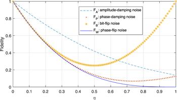
Apparently, one can see that the fidelities depend on the parameters of the initial states and the decoherence rates. Specifically, a case is given in figure 2, as we assume that ${\alpha }_{1}={\alpha }_{2}={\beta }_{1}={\beta }_{2}=1/\sqrt{2}$, η = η_A = η_P = η_B = η_W. In this case, as the decoherence rate η increases, F_A is the highest compared to F_P, F_B, F_W, until η > 0.6423, F_B is the highest. In addition, F_B decreases initially and then increases as the decoherence rate η increases. Figure 3 shows the fidelities with different coefficients of the initial states and decoherence rates.

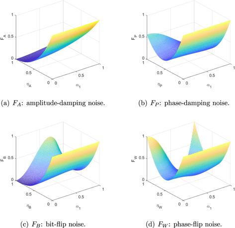
In figures 3(a), (c), it is clearly that F_A and F_B decrease as the decoherence rates η_A and η_B increase. While in the phase-damping and phase-flip noisy environments, F_P and F_W decrease initially and then increase as the decoherence rates η_P and η_W increase (see figures 3(b), 3(d)).

Figure 2.

New window|Download| PPT slide
Figure 2.The trend of the fidelities of the output states with the change of the decoherence rate η in four types of noisy environments.

Figure 3.

New window|Download| PPT slide
Figure 3.Effects of four kinds of noises on M-QT scheme are visualized through variation of fidelities (F_A, F_P, F_B and F_W) under the situation ${\alpha }_{1}={\alpha }_{1},{\alpha }_{2}=1/2,{\beta }_{2}=\sqrt{3}/2$.

3. Multi-output QT of an m-qubit GHZ-class state and an (m+1)-qubit GHZ-class state

The idea can be further extend to a more general situation where an m-qubit GHZ-class state and an (m+1)-qubit GHZ-class state are teleported from one sender to two distant receivers respectively. The messages (i.e. the m-qubit and the (m+1)-qubit GHZ-class states) of two receivers respectively are given by(12)$\begin{eqnarray}\left\{\begin{array}{l}| {\chi }_{1}^{m}\rangle ={\left({\alpha }_{1}| 0{\rangle }^{\otimes m}+{\beta }_{1}| 1{\rangle }^{\otimes m}\right)}_{1,2,\cdots ,m}\\ | {\chi }_{2}^{m+1}\rangle ={\left({\alpha }_{2}| 0{\rangle }^{\otimes (m+1)}+{\beta }_{2}| 1{\rangle }^{\otimes (m+1)}\right)}_{m+1,m+2,\cdots ,2m+1},\end{array}\right.\end{eqnarray}$where the parameters α_i, β_i satisfy the normalized condition ∣α_i∣² + ∣β_i∣² = 1(i = 1, 2). The shared quantum channel is a five-qubit entangled state $| {\rm{\Psi }}{\rangle }_{{A}_{1}{A}_{2}{{BC}}_{1}{C}_{2}}$ mentioned as equation (2), while the composite system turns to(13)$\begin{eqnarray}\begin{array}{rcl}| {\rm{\Omega }}^{\prime\prime} {\rangle }_{T} & = & | {\chi }_{1}^{m}{\rangle }_{\mathrm{1,2},\cdots ,m}\otimes | {\chi }_{2}^{m+1}{\rangle }_{m+1,m+2,\cdots ,2m+1}\otimes | {\rm{\Psi }}{\rangle }_{{A}_{1}{A}_{2}{{BC}}_{1}{C}_{2}}\\ & = & {\left({\alpha }_{1}| 0{\rangle }^{\otimes m}+{\beta }_{1}| 1{\rangle }^{\otimes m}\right)}_{1,2,\cdots ,m}\\ & & \otimes {\left({\alpha }_{2}| 0{\rangle }^{\otimes (m+1)}+{\beta }_{2}| 1{\rangle }^{\otimes (m+1)}\right)}_{m+1,m+2,\cdots ,2m+1}\\ & & \otimes \displaystyle \frac{1}{2}\left(| 00000\rangle +| 01011\rangle +| 10100\rangle \right.\\ & & {\left.+| 11111\rangle \right)}_{{A}_{1}{A}_{2}{{BC}}_{1}{C}_{2}}.\end{array}\end{eqnarray}$

We detail m with two cases here for odd and even values: (i) m is odd. Alice performs m BSMs on the particles (1, A₁), (m + 1, A₂), (2, 3), ⋯ ,(m − 1, m), (m + 2, m + 3), ⋯ ,(2m − 1, 2m), and an H operation on the remaining one particle H(2m + 1); (ii) m is even. Alice performs m BSMs on the particles (1, A₁), (m + 1, A₂), (2, 3), ⋯ ,(m − 2, m − 1), (m + 2, m + 3), ⋯ ,(2m, 2m + 1), and an H operation on the remaining one particle H(m).

After sender Alice conveys the classical information to receivers Bob and Charlie, each receiver creates the auxiliary particles with initial state $| 0{\rangle }_{{o}_{1}{o}_{2}\cdots {o}_{m-1}}^{\otimes (m-1)}(o=b,c)$ and performs CNOT operation with required number of ancillary particles, respectively. Finally, following the same rule, receivers apply appropriate unitary operations to recover the target states.

4. Conclusion

In summary, we propose the schemes to teleport many GHZ-class states with one sender to multiple receivers synchronously, and generalize it to the multi-qubit state system. Note that we have experimentally realized the particular case of the proposed scheme using IBM Q platform. To teleport an m-qubit and an (m+1)-qubit GHZ-class states, sender has to perform BSMs m times and a Hadamard operation on the remaining particle. After her measurements, she tells receivers her results. Then each receiver introduces the auxiliary particles and performs CNOT operations the required number of ancillary qubits, finally takes the unitary operation according to the measurement results. Further, we assessed our first scheme performance in four types of noisy environments, and calculate the fidelities of the output states. We expect our work may offer some light to multiparty multicast quantum communications.

Reference View Option By original order
By published year
By cited within times
By Impact factor

[1]Bennett C H Brassard G Crépeau C Jozsa R Peres A Wootters W K 1993 Phys. Rev. Lett. 70 1895 1899
DOI:10.1103/PhysRevLett.70.1895 [Cited within: 1]

[2]Bouwmeester D Pan J W Mattle K Eibl M Weinfurter H Zeilinger A 1997 Nature 390 575 579
DOI:10.1038/37539 [Cited within: 1]

[3]Agarwal P Pati A 2006 Phys. Rev. A 74 062320
DOI:10.1103/PhysRevA.74.062320 [Cited within: 1]

[4]Guan S 2010 Int. J. Quantum Inf. 8 1411
DOI:10.1142/S0219749910006964 [Cited within: 1]

[5]Chuang L D Liang C Z 2007 Commun. Theor. Phys. 47 464
DOI:10.1088/0253-6102/47/3/017 [Cited within: 1]

[6]Nandi K Mazumdar C 2014 Int. J. Theor. Phys. 53 1322 1324
DOI:10.1007/s10773-013-1928-1 [Cited within: 1]

[7]Li D F Wang R J Baagyere E 2019 Quantum Inf. Process. 18 1471
[Cited within: 1]

[8]Bei Z et al. 2002 Commun. Theor. Phys. 38 537
DOI:10.1088/0253-6102/38/5/537 [Cited within: 2]

[9]Long L R Li H W Zhou P Fan C Yin C L 2011 Sci. China Phys. Mech. Astron 54 484 490
DOI:10.1007/s11433-011-4246-8 [Cited within: 1]

[10]Yu Y Zha X W Li W 2017 Quantum Inf. Process 16 41
DOI:10.1007/s11128-016-1500-z [Cited within: 1]

[11]Choudhury B S Dhara A 2018 Int. J. Theor. Phys. 57 1 8
DOI:10.1007/s10773-017-3534-0 [Cited within: 1]

[12]Wei J H 2018 Int. J. Theor. Phys. 57 3104 3111
DOI:10.1007/s10773-018-3828-x [Cited within: 1]

[13]Li H J Chen X B Wang Y L 2019 Quantum Inf. Process. 18 266
DOI:10.1007/s11128-019-2374-7 [Cited within: 1]

[14]Zhou R Qian C Ian H 2019 IEEE Access 7 42445 42449
DOI:10.1109/ACCESS.2019.2907963 [Cited within: 1]

[15]Sun S Li L Zhang H 2020 Int. J. Theor. Phys. 59 1017 1030
DOI:10.1007/s10773-019-04367-2 [Cited within: 1]

[16]Yang L Liu Y C Li Y S 2020 Chin. Phys. B 29 060301
DOI:10.1088/1674-1056/ab84de [Cited within: 1]

[17]Hu X M et al. 2019 Quantum Eng. 1 e13
DOI:10.1002/que2.12

[18]Li M S et al. 2020 Sci. China Phys. Mech. Astron 63 280312
DOI:10.1007/s11433-020-1562-4

[19]Roa L et al. 2019 Front. Phys. 14 61602
DOI:10.1007/s11467-019-0939-7

[20]Chang C R et al. 2020 AAPPS Bulletin 30 9 22


[21]Yan Z et al. 2021 Fundam. Res. 1 43 49
DOI:10.1016/j.fmre.2020.11.005

[22]Britt B C 2020 Quantum Eng. 2 e29
DOI:10.1002/que2.29 [Cited within: 1]

[23]Chatterjee Y et al. 2020 Quantum Inf. Process. 19 31
DOI:10.1007/s11128-019-2527-8 [Cited within: 1]

[24]Huang N N Huang W H Li C M 2020 Sci. Rep. 10 3093
DOI:10.1038/s41598-020-60061-y [Cited within: 1]

[25]Baishya S k R A et al. 2020 Quantum Inf. Process. 19 87
DOI:10.1007/s11128-020-2586-x [Cited within: 1]

[26]Huang W J et al. 2020 Quantum Eng. 2 e45
[Cited within: 1]

[27]Zhukov A A Remizov S V Pogosov W V Lozovik Y E 2018 Quantum Inf. Process. 17 223
DOI:10.1007/s11128-018-2002-y [Cited within: 1]

[28]Viyuela O 2018 NPJ Quantum Inf. 4 10
DOI:10.1038/s41534-017-0056-9 [Cited within: 1]

[29]García-Martín D Sierra G 2018 J. Appl. Math. Phys. 6 1460
DOI:10.4236/jamp.2018.67123 [Cited within: 1]

[30]Swain M Rai A Behera B K Panigrahi P K 2019 Quantum Inf. Process. 18 218
DOI:10.1007/s11128-019-2331-5 [Cited within: 1]

[31]Chatterjee Y Devrari V Behera B K Panigrahi P K 2019 Quantum Inf. Process. 19 31
DOI:10.1007/s11128-019-2527-8 [Cited within: 1]

[32]Rajiuddin S K Baishya A Behera B K Panigrahi P K 2020 Quantum Inf. Process. 19 87
DOI:10.1007/s11128-020-2586-x [Cited within: 1]

[33]Behera B K Reza T Gupta A Panigrahi P K 2019 Quantum Inf. Process. 18 328
DOI:10.1007/s11128-019-2436-x [Cited within: 1]

[34]Liang X T 2003 Commun. Theor. Phys. 39 537 542
DOI:10.1088/0253-6102/39/5/537 [Cited within: 1]