Ji-Guo Wang^,1,2, Lin-Qi Guo^1,2, Ya-Fei Song¹¹Department of Mathematics and Physics, Shijiazhuang TieDao University, Shijiazhuang 050043, China
²Institute of Applied Physics, Shijiazhuang TieDao University, Shijiazhuang 050043, China

Received:2021-03-4Revised:2021-05-21Accepted:2021-05-24Online:2021-06-25


Abstract
We study the quantum coherence and ground-state phase transition of a four-chain Bose–Hubbard model with the long-range interaction. In a special four-chain Bose–Hubbard model, i.e., each chain only has one optical potential, four types of the ground-state phases are discovered. The effects of the disorder, the on-site interaction and the long-range interaction on the quantum coherence are studied. For the system without the long-range interaction, the quantum coherence changes from one periodic oscillation to two periodic oscillations as the on-site interaction increases. By considering the long-range interaction, the quantum coherence goes back to one periodic oscillation again. The on-site interaction itself suppresses the quantum coherence, both the on-site interaction and long-range interaction together enhance the quantum coherence with the weak disorder. If the disorder strength is increased beyond a critical value, they start to suppress the quantum coherence. In a regular four-chain Bose–Hubbard model, i.e., each chain has many optical potentials, the ground-state phase transitions are obtained by using the cluster Gutzwiller mean-field method. Exotic ground-state phases are found, i.e., superfluid phase, integer Mott insulator phase, supersolid phase and loophole insulator phase. The combination of the loophole insulator phase and the supersolid phase expands the lobes with the half-integer filling per site for the small ratio β = t_∥/t_⊥.
Keywords： Bose–Hubbard model;quantum coherence;ground-state phase transition


PDF (926KB)MetadataMetricsRelated articlesExportEndNote|Ris|BibtexFavorite
Cite this article
Ji-Guo Wang, Lin-Qi Guo, Ya-Fei Song. Quantum coherence and ground-state phase transition in a four-chain Bose–Hubbard model. Communications in Theoretical Physics, 2021, 73(8): 085702- doi:10.1088/1572-9494/ac0427

1. Introduction

Ultracold bosonic atoms trapped in an optical lattice, which can be described by the celebrated Bose–Hubbard (BH) model. The BH model includes the nearest-neighbor or long-range interactions is called the extended BH model. The interactions and disorder in the BH or extended BH model can be tuned independently in an experiment, which results in many rich phenomena in the condensed matter and statistical physics [1–5]. For the long-range interaction, it has been studied in the ultracold particles with the large magnetic or electronic dipole moments. The long-range interaction decays algebraically with the particles distance R, i.e., 1/R^α (α = 3). The BH model with long-range interactions has also been investigated in many previous works [6–10].

The superfluid (SF) phase and the Mott insulator (MI) phase exist when the BH model has only the on-site interaction [11]. By considering the disorder, the gapless Bose glass (BG) phase is found. The BG phase always intervenes between the SF phase and MI phase, it has finite compressibility and absences of off-diagonal long-range order [12–15]. For the extended BH model, the nearest-neighbor or long-range interaction noticeably enriches the ground-state phase diagram. The ground-state phases can be obtained by using mean-field theory, Gutzwiller method, quantum Monte-Carlo, variational Monte-Carlo, and exact diagonalization in the one-dimensional (1D), two-dimensional (2D), and three-dimensional (3D) systems. In addition to the ground-state phases above, the density wave (DW) phase, the checkboard (CB) phase and the supersolid (SS) phase have also been reported [16–23].

In this paper, we study the quantum coherence and ground-state phase transition of a four-chain BH model with the long-range interaction. In a special four-chain BH model, four types of ground-state phases are classified by the atomic number. The effects of the disorder, the on-site interaction and the long-range interaction on the quantum coherence are also discussed. For the system without a long-range interaction, the quantum coherence changes from one periodic oscillation to two periodic oscillations as the on-site interaction increases. By considering the long-range interaction, the quantum coherence goes back to one periodic oscillation again. The on-site interaction itself suppresses the quantum coherence, both the on-site interaction and long-range interaction together enhance the quantum coherence with the weak disorder. If the disorder strength is increased beyond a critical value, they start to suppress the quantum coherence. In a regular four-chain BH model, the ground-state phase transitions are studied. Exotic ground-state phases are found, i.e., SF phase, MI phase, SS phase and loophole insulator (LI) phase. When the ratio β = t_∥/t_⊥ is very small, the combination of both the LI and the SS phases expands the lobes with the half-integer filling per site.

The paper is organized as follows. In section 2 we introduce the four-chain BH model with the long-range interaction. In section 3 we present the ground-state phases and quantum coherence in the special four-chain BH model. In section 4 we display the quantum phase transitions in the regular four-chain BH model. A brief summary is included in section 5.

2. Model and Hamiltonian

We discuss the quantum coherence and ground-state phase transition in a four-chain BH model with the long-range interaction, the Hamiltonian can be written as follows:(1)$\begin{eqnarray}\begin{array}{rcl}\hat{H} & = & -{t}_{\parallel }\displaystyle \sum _{\langle {ij}\rangle ,\sigma }^{M}({\hat{b}}_{i,\sigma }^{\dagger }{\hat{b}}_{j,\sigma }+{\rm{H}}.{\rm{c}}.)-{t}_{\perp }\displaystyle \sum _{i,\sigma }^{M}({\hat{b}}_{i,\sigma }^{\dagger }{\hat{b}}_{i,\sigma +1}+{\rm{H}}.{\rm{c}}.)\\ & & +\displaystyle \frac{U}{2}\displaystyle \sum _{i,\sigma }^{M}{n}_{i,\sigma }({n}_{i,\sigma }-1)+\displaystyle \frac{V}{{L}^{3}}\displaystyle \sum _{i,\sigma \ne {\sigma }^{{\prime} }}^{M}{n}_{i,\sigma }{n}_{i,{\sigma }^{{\prime} }}\\ & & -\displaystyle \sum _{i,\sigma }^{M}{\epsilon }_{\sigma }({n}_{i,\sigma +1}-{n}_{i,\sigma })-\mu \displaystyle \sum _{i,\sigma }^{M}{n}_{i\sigma },\end{array}\end{eqnarray}$where Σ = 1, 2, …, M (M = 4) denotes the Σ-th chain of the four-chain BH model. ${\hat{b}}_{i,\sigma }^{\dagger }({\hat{b}}_{i,\sigma })$ is the bosonic creation (annihilation) operator and ${n}_{i,\sigma }={\hat{b}}_{i,\sigma }^{\dagger }{\hat{b}}_{i,\sigma }$ is the number operator at site i of the Σ chain. Here ⟨ ⋯ ⟩ denotes the nearest neighboring sites in the same chain and $L=| \sigma -{\sigma }^{{\prime} }| $ is the distance between the chain Σ and the chain Σ′. The parameters t_∥ and t_⊥ are the intra- and inter-chain nearest-neighbor tunnelling strengths, respectively. U is the on-site repulsive interaction and V is the long-range repulsive interaction. The disorder can be introduced into the model via the random fluctuation of ε_Σ, here, we set ε_Σ = ε. The chemical potential μ determines the particle filling.

3. Ground-state phase and quantum coherence in a special four-chain BH model

If each chain of the four-chain BH model only has one optical potential, we call the model the special four-chain BH model. The Hamiltonian of the special four-chain BH can be obtained from the equation (1),(2)$\begin{eqnarray}\begin{array}{rcl}\hat{H} & = & -{t}_{\perp }\displaystyle \sum _{\sigma }^{M}({\hat{b}}_{\sigma }^{\dagger }{\hat{b}}_{\sigma +1}+{\rm{H}}.{\rm{c}}.)+\displaystyle \frac{U}{2}\displaystyle \sum _{\sigma }^{M}{n}_{\sigma }({n}_{\sigma }-1)\\ & & +\displaystyle \frac{V}{{L}^{3}}\displaystyle \sum _{\sigma \ne {\sigma }^{{\prime} }}^{M}{n}_{\sigma }{n}_{{\sigma }^{{\prime} }}-\epsilon \displaystyle \sum _{\sigma }^{M}({n}_{\sigma +1}-{n}_{\sigma }).\end{array}\end{eqnarray}$The inter-chain nearest-neighbor tunnelling strength t_⊥ = t and the total particle number ${\sum }_{\sigma =1}^{4}{n}_{\sigma }=N=32$. In the Fock space, the Schrödinger equation can be written as $\hat{H}| {\rm{\Psi }}\rangle =E| {\rm{\Psi }}\rangle $. The basis of Fock state is ∣n₁, n₂, n₃⟩ = ∣n₁, n₂, n₃, N − n₁ − n₂ − n₃⟩, here n₁ = 1, 2, 3, …, N − 1, N, n₂ = 1, 2, 3,…,N − n₁ − 1, N − n₁, n₃ = 1, 2, 3,…,N − n₁ − n₂ − 1, N − n₁ − n₂ and n₄ = N − n₁ − n₂ − n₃. The wave function can be expanded as $| {\rm{\Psi }}\rangle ={{\rm{\Sigma }}}_{{n}_{1},{n}_{2},{n}_{3}}{\psi }_{{n}_{1},{n}_{2},{n}_{3}}| {n}_{1},{n}_{2},{n}_{3}\rangle $, we obtain(3)$\begin{eqnarray}\begin{array}{l}(E-{E}_{{n}_{1},{n}_{2},{n}_{3}})=-{t}_{\perp }{M}_{{n}_{1}+1,{n}_{2}-1,{n}_{3}}| {n}_{1}+1,{n}_{2}-1,{n}_{3}\rangle \\ \quad -{t}_{\perp }{M}_{{n}_{1}-1,{n}_{2}+1,{n}_{3}}| {n}_{1}+1,{n}_{2}-1,{n}_{3}\rangle \\ \quad -{t}_{\perp }{M}_{{n}_{1},{n}_{2}+1,{n}_{3}-1}| {n}_{1},{n}_{2}+1,{n}_{3}-1\rangle \\ \quad -{t}_{\perp }{M}_{{n}_{1},{n}_{2}-1,{n}_{3}+1}| {n}_{1},{n}_{2}-1,{n}_{3}+1\rangle \\ \quad -{t}_{\perp }{M}_{{n}_{1},{n}_{2},{n}_{3}+1}| {n}_{1},{n}_{2},{n}_{3}+1\rangle \\ \quad -{t}_{\perp }{M}_{{n}_{1},{n}_{2},{n}_{3}-1}| {n}_{1},{n}_{2},{n}_{3}-1\rangle ,\end{array}\end{eqnarray}$where ${E}_{{n}_{1},{n}_{2},{n}_{3}}=U[{n}_{1}^{2}+{n}_{2}^{2}+{n}_{3}^{2}$ - $\tfrac{{N}^{2}}{2}+{n}_{1}{n}_{2}+{n}_{1}{n}_{3}\,+{n}_{2}{n}_{3}-N({n}_{1}+{n}_{2}+{n}_{3})]+V({n}_{1}{n}_{2}+{{Nn}}_{3}-{n}_{1}{n}_{3}-{n}_{1}^{2})$ + $\tfrac{V}{8}({n}_{1}{n}_{3}+{n}_{2}N-{n}_{1}{n}_{2}-{n}_{2}^{2}-{n}_{2}{n}_{3})$ + $\tfrac{V}{27}({n}_{1}N-{n}_{1}^{2}-{n}_{1}{n}_{2}-{n}_{1}{n}_{3})\,-\epsilon (N-{n}_{3}-{n}_{2}-2{n}_{1})$, ${M}_{{n}_{1}+1,{n}_{2}-1,{n}_{3}}=\sqrt{({n}_{1}+1){n}_{2}}$, ${M}_{{n}_{1}-1,{n}_{2}+1,{n}_{3}}$ = $\sqrt{{n}_{1}({n}_{2}+1)}$, ${M}_{{n}_{1},{n}_{2}+1,{n}_{3}-1}=\sqrt{({n}_{2}+1){n}_{3}}$, ${M}_{{n}_{1},{n}_{2}-1,{n}_{3}+1}\,=\sqrt{{n}_{2}({n}_{3}+1)}$, ${M}_{{n}_{1}+1,{n}_{2},{n}_{3}+1}\,=\sqrt{({n}_{3}+1)(N-{n}_{1}-{n}_{2}-{n}_{3})}$, ${M}_{{n}_{1}-1,{n}_{2},{n}_{3}-1}$ = $\sqrt{{n}_{3}(N-{n}_{1}-{n}_{2}-{n}_{3}+1)}$.

We can evaluate the eigenenergies and eigenfunctions from the equation (3) by using the exact diagonalization method [24], the dimension of this space is $D=\tfrac{(N+M-1)!}{N!(M-1)!}=6545$ (total particle number N= 32 and chain number M = 4). The ground-state phases and quantum coherences of the special four-chain BH model can be discussed.

3.1. Ground-state phases

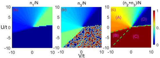
We first study the ground-state phases of a special four-chain BH model without the disorder ϵ = 0. The ground-state phase diagrams spanned by the on-site interaction U and long-range interaction V are plotted in figure 1, four types of ground-state phases are classified by the particle number n_Σ/N, i.e., the (A)–(D) phases in figure 1(c). In the (A) phase, the particles number of ${n}_{1}+{n}_{3}=\lfloor \bar{n}\rfloor $ with $\bar{n}=\tfrac{(8V-216U)N}{216U-235V}$, where ⌊…⌋ donates the integer number. In the (B) phase, the particle number of n₂ + n₃ = N (n₂ = n₃ = N/2). In the (C) phase, the particle number of n₂ + n₃ = N (n₂ = N or n₃ = N). In the (D) phase, the particle number of n₂ + n₃ = 0 (n₁ = n₄ = N/2).

Figure 1.

New window|Download| PPT slide
Figure 1.The ground-state phase diagrams are classified by the atomic number n_Σ/N as a function of U and V, i.e., n₁/N, n₂/N and (n₂ + n₃)/N in (a)–(c), respectively, four types of ground-state phase are shown. The dotted lines in (c) are the analytical solutions of the minimization of equation (5).


For the fixed total particle number, the global on-site energy UN(N − 1)/2 is conserved. The equation (2) can be rewritten as(4)$\begin{eqnarray}\begin{array}{rcl}\hat{H} & = & -t\displaystyle \sum _{\sigma }^{M}({\hat{b}}_{\sigma }^{\dagger }{\hat{b}}_{\sigma +1}+{\rm{H}}.{\rm{c}}.)\\ & & +(V-U)({n}_{1}{n}_{2}+{n}_{2}{n}_{3}+{n}_{3}{n}_{4})\\ & & +\left(\displaystyle \frac{V}{8}-U\right)({n}_{1}{n}_{3}+{n}_{2}{n}_{4})+\left(\displaystyle \frac{V}{27}-U\right)({n}_{1}{n}_{4}),\end{array}\end{eqnarray}$the Fock states ∣n₁, n₂, n₃⟩ are the eigenstates of $\hat{H}$ in equation (4), and the corresponding energy is ${E}_{{n}_{1},{n}_{2},{n}_{3}}^{{\prime} }$. We can minimizes the energy ${E}_{{n}_{1},{n}_{2},{n}_{3}}^{{\prime} }$ (t = 0) by using the variational method,(5)$\begin{eqnarray}\begin{array}{l}\displaystyle \frac{\partial {E}_{{n}_{1},{n}_{2},{n}_{3}}^{{\prime} }}{\partial {n}_{2}}=(V-U)({n}_{1}-2{n}_{2}-{n}_{4})+\left(\displaystyle \frac{V}{8}-U\right)\\ (2{n}_{4}-N)+\left(\displaystyle \frac{V}{27}-U\right)({n}_{2}+{n}_{3}-N),\\ \displaystyle \frac{\partial {E}_{{n}_{1},{n}_{2},{n}_{3}}^{{\prime} }}{\partial {n}_{3}}=(V-U)({n}_{4}-2{n}_{3}-{n}_{1})+\left(\displaystyle \frac{V}{8}-U\right)\\ (2{n}_{1}-N)+\left(\displaystyle \frac{V}{27}-U\right)({n}_{2}+{n}_{3}-N).\end{array}\end{eqnarray}$

The regions of the four types of the ground-state phases in figure 1(c) can be obtained from the minimization of E(n₁, n₂, n₃) in equation (5). The (A) phase in the region of V ≤ 16/9U when U > 0, and V ≥ 27U when U < 0, the (B) phase in the region of 27U ≤ V ≤ 235/216U when U < 0, the (c) phase in the region of V ≥ 27U when U > 0 and V ≥ 235/216U when U < 0 and the (D) phase in the region 16/9U ≤ V ≤ 27U when U > 0.

3.2. Quantum coherence

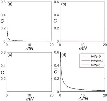
In a pure BH model, the interaction can suppress the particle number fluctuation and quantum coherence, the system starts from the coherent state to the Fock state as the interaction increases. The coherent and Fock states correspond to the conventional SF and MI phases, respectively. When considering the disorder, the interaction and disorder together enhance the quantum coherence [25, 26]. where they strength are comparable. The quantum coherence of a simple model can well reflect the details of the quantum phase diagram of the full BH model. In this section, we will discuss the quantum coherence in a special disordered four-chain BH model with a long-range interaction. The quantum coherence is defined as $C=\tfrac{1}{N}\sum \langle {b}_{\sigma }^{\dagger }{b}_{\sigma +1}\rangle $ and the expectation value can be obtained by averaging C, i.e., $\bar{C}=\tfrac{1}{2{\rm{\Delta }}}{\int }_{-{\rm{\Delta }}}^{{\rm{\Delta }}}C{\rm{d}}\epsilon $, which means the quantum coherence C in the regime of ε ∈ [−Δ, Δ]. If C > 0 or $\bar{C}\gt 0$, the system in the coherent state, that corresponds to the SF phase, accordingly, C → 0 or $\bar{C}\to 0$, the system in the decoherent state, that corresponds to the MI phase.

The quantum coherence C ($\bar{C}$) as a function of ε/tN is shown in figure 2, and the on-site interaction U = 0. The long-range interactions in (a)–(c) are V/tN = 0, 0.3 and 1, respectively. The quantum coherence C quickly monotonic decreases as the disorder ε increases in figure 2(a), it shows that the noninteracting particles continuous tunnelling between the chains when the disorder ε is smaller than the tunnelling strength t. Considering the long-range interaction, the quantum coherence C is severely suppressed within the whole regime of ε, the system in a decoherent state, one can be seen in figure 2(b) and (c). We next study quantum coherence C ($\bar{C}$) with the weak on-site interaction U/tN = 1 in figure 3, the parameters are the same with figure 2 shown. The quantum coherence C shows the periodic oscillation character with V = 0, and the peaks locate in the certain disorder values ε*, as shown in figure 3(a). Figure 3(b) and (c) show that the periodic oscillation character of C is inhibited with V = 0.3 and V = 1, respectively. However, in the regime of the weak disorder, the values of $\bar{C}$ with V = 0.3 are larger than $\bar{C}$ with V = 0 in figure 3(d).

Figure 2.

New window|Download| PPT slide
Figure 2.The quantum coherence C as a function of ε/tN with U/tN = 0, the long-range interactions V/tN = 0, 0.3 and 1 in (a)–(c), respectively. (d) Is the corresponding $\bar{C}$ as a function of Δ/tN.

Figure 3.

New window|Download| PPT slide
Figure 3.The quantum coherence C as a function of ε/tN with U/tN = 1, the long-range interactions V/tN = 0, 0.3 and 1 in (a)–(c), respectively. (d) Is the corresponding $\bar{C}$ as a function of Δ/tN.


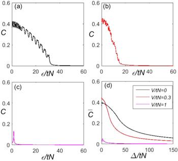
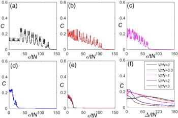
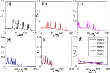
The quantum coherences C ($\bar{C}$) exhibit an interesting physical phenomena with the large on-site interactions U/tN = 4 and 9.95 in figures 4 and 5, respectively. In figures 4(a) and 5(a), the peak of C at ε* with V/tN = 0. Unlike the quantum coherence in the previous works [25, 26], the quantum coherence in our system has two periodic oscillations. As the disorder increases, the value of C in the first periodic oscillation decreases with the disorder increasing. If the disorder strength is increased beyond a critical value, the quantum coherence C transients from the first periodic oscillation to the second periodic oscillation, and the peaks of the second periodic oscillation instantly enhanced. Each peak is divided into two parts. When considering the small long-range interaction V/tN = 0.3 in figures 4(b) and 5(b), the quantum coherence C of the first periodic oscillation shows the completely opposite characteristics comparing with case in figures 4(a) and 5(a) shown, they increase as the disorder strength increases. For the larger long-range interaction, the quantum coherence C becomes one periodic oscillation and is seriously suppressed. From figures 4 and 5, we can obtain that the on-site interaction itself suppresses the quantum coherence, both the on-site interaction and long-range interaction together enhance the quantum coherence with the weak disorder. If the disorder strength is increased beyond a critical value, they start to suppress the quantum coherence.

Figure 4.

New window|Download| PPT slide
Figure 4.The quantum coherence C ($\bar{C}$) as a function of ε/tN with U/tN = 4, the long-range interactions V/tN = 0, 0.3, 1, 2, and 3 in (a)–(e), respectively. (f) Is the corresponding $\bar{C}$ as a function of Δ/tN.

Figure 5.

New window|Download| PPT slide
Figure 5.The quantum coherence C ($\bar{C}$) as a function of ε/tN with U/tN = 9.95, the long-range interactions V/tN = 0, 0.3, 1, 2, and 3 in (a)–(e), respectively. (f) Is the corresponding $\bar{C}$ as a function of Δ/tN.


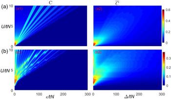
The complete pictures of the quantum coherence C or $\bar{C}$ as a function of ε/tN or Δ/tN and U/tN are shown in in figure 6(a) with V/tN = 0 and figure 6(b) with V/tN = 1 are plotted. Figure 6(a) shows that for large U without long-range interaction, the contours of C change from one periodic oscillation to two periodic oscillations and $\bar{C}$ bend to the up site when Δ/tN increases from zero. For a fixed value of U, away from the positions of the peaks, $\bar{C}$ changes slowly, vice versa, $\bar{C}$ quickly increases when approaching the peaks. Considering the long-range interaction V/tN = 1, C goes back to one periodic oscillation again, and the system in the coherent state when U ≥ V. The on-site interaction U itself suppresses $\bar{C}$, both the on-site interaction U and long-range interaction V together enhance $\bar{C}$ with the weak disorder Δ ≃ 0, which can be found in figure 6(b2). Compared with figure 6(a2) and (b2), we find that the regime of the coherent state is larger than the system without the long-range interaction.

Figure 6.

New window|Download| PPT slide
Figure 6.A contours plot of C or $\bar{C}$ as a function of ε/tN and U/tN in (a) with V/tN = 0 and (b) with V/tN = 1.


The peak value ε* of the periodical oscillation can be obtained analytically by the variational analyzing of the state energy ${E}_{{n}_{1},{n}_{2},{n}_{3}}^{{\prime} }$,(6)$\begin{eqnarray}\begin{array}{l}\displaystyle \frac{\partial {E}_{{n}_{1},{n}_{2},{n}_{3}}^{{\prime} }}{\partial {n}_{2}}=(V-U)({n}_{1}-2{n}_{2}-{n}_{4})\\ \quad +\left(\displaystyle \frac{V}{8}-U\right)(2{n}_{4}-N)\\ \quad +\left(\displaystyle \frac{V}{27}-U\right)({n}_{2}+{n}_{3}-N)-\epsilon ,\\ \displaystyle \frac{\partial {E}_{{n}_{1},{n}_{2},{n}_{3}}^{{\prime} }}{\partial {n}_{3}}=(V-U)({n}_{4}-2{n}_{3}-{n}_{1})\\ \quad +\left(\displaystyle \frac{V}{8}-U\right)(2{n}_{1}-N)\\ \quad +\left(\displaystyle \frac{V}{27}-U\right)({n}_{2}+{n}_{3}-N)-\epsilon .\end{array}\end{eqnarray}$The value of ε* is(7)$\begin{eqnarray}{\epsilon }^{* }=({n}_{2}+{n}_{3})\left(U-\displaystyle \frac{235V}{216}\right)+\left(\displaystyle \frac{V}{27}-U\right)N,\end{eqnarray}$where n₂ + n₃ = 0, 1, 2, …, N.

4. Quantum phase transition in a regular four-chain BH model

We find that the on-site interaction U and long-range interaction V play an important role on the ground-state phases and the quantum coherence of the special four-chain BH model. In order to show the effects of the long-range interaction on the regular four-chain BH model, we study the quantum phase transition in a regular four-chain BH model by using the cluster Gutzwiller mean-field method [27, 28]. Here, the cluster Gutzwiller mean-field method keeps the intra-chain tunnelling terms and only decouples the inter-chain tunnelling terms, which is different from the single-site mean-field method. In the mean-field approximation, the inter-cluster tunnelling terms can be decoupled as(8)$\begin{eqnarray}\begin{array}{rcl}{\hat{b}}_{i\sigma }^{\dagger }{\hat{b}}_{j\sigma } & \approx & {\hat{b}}_{i\sigma }^{\dagger }\langle {\hat{b}}_{j\sigma }\rangle +\langle {\hat{b}}_{i\sigma }^{\dagger }\rangle {\hat{b}}_{j\sigma }-\langle {\hat{b}}_{i\sigma }^{\dagger }\rangle \langle {\hat{b}}_{j\sigma }\rangle \\ & = & {\hat{b}}_{i\sigma }^{\dagger }{\phi }_{j\sigma }+{\phi }_{i\sigma }^{* }{\hat{b}}_{j\sigma }-{\phi }_{i\sigma }^{* }{\phi }_{j\sigma },\end{array}\end{eqnarray}$we substitute equations (7) into (1), the mean-field single-cluster Hamiltonian is obtained,(9)$\begin{eqnarray}\begin{array}{l}{\hat{{H}_{i}}}^{{mf}}=-{t}_{\parallel }\displaystyle \sum _{i=j\pm 1,\sigma }({\hat{b}}_{i\sigma }^{\dagger }{\phi }_{j\sigma }+{\phi }_{i\sigma }^{* }{\hat{b}}_{j\sigma }-\mathrm{Re}[{\phi }_{i\sigma }^{* }{\phi }_{j\sigma }])\\ \quad -{t}_{\perp }\displaystyle \sum _{i,\sigma }({\hat{b}}_{i,\sigma }^{\dagger }{\hat{b}}_{i,\sigma +1}+{\rm{H}}.{\rm{c}}.)+\displaystyle \frac{U}{2}\displaystyle \sum _{i,\sigma }{n}_{i,\sigma }({n}_{i,\sigma }-1)\\ \quad +\displaystyle \frac{V}{{L}^{3}}\displaystyle \sum _{i,\sigma \ne {\sigma }^{{\prime} }}{n}_{i,\sigma }{n}_{i,{\sigma }^{{\prime} }}-\mu \displaystyle \sum _{i,\sigma }{n}_{i\sigma }.\end{array}\end{eqnarray}$

The state for the whole system can be expressed as a product state of single-cluster states with the cluster mean-field method,(10)$\begin{eqnarray}| {\rm{\Phi }}\rangle =\prod _{j}| {\rm{\Psi }}{\rangle }_{j}.\end{eqnarray}$The j-th cluster state is $| {\rm{\Psi }}{\rangle }_{j}={\sum }_{{n}_{1}=0}^{{N}_{\max }}{\sum }_{{n}_{2}=0}^{{N}_{\max }}{\sum }_{{n}_{3}=0}^{{N}_{\max }}$ ${\sum }_{{n}_{4}=0}^{{N}_{\max }}{f}_{{n}_{1},{n}_{2},{n}_{3},{n}_{4}}^{j}| {n}_{1},{n}_{2},{n}_{3},{n}_{4}{\rangle }_{j},$ where ∣n₁, n₂, n₃, n₄⟩ is the j-th cluster state basis, ${f}_{{n}_{1},{n}_{2},{n}_{3},{n}_{4}}^{j}$ are the corresponding probability amplitudes and N_max (N_max = 4) is the truncation of the maximum particle number. The equation (8) is substituted into the j-th eigenequation equation ${\widehat{H}}_{j}^{{mf}}| {\rm{\Psi }}{\rangle }_{j}={E}_{j}| {\rm{\Psi }}{\rangle }_{j}$, we obtain(11)$\begin{eqnarray}\begin{array}{l}{E}_{j}{f}_{{n}_{1},{n}_{2},{n}_{3},{n}_{4}}^{j}=-{t}_{\parallel }{\phi }_{j1}\sqrt{{n}_{1}+1}{f}_{{n}_{1}+1,{n}_{2},{n}_{3},{n}_{4}}^{j}\\ -{t}_{\parallel }{\phi }_{j1}^{* }\sqrt{{n}_{1}}{f}_{{n}_{1}-1,{n}_{2},{n}_{3},{n}_{4}}^{j}-{t}_{\parallel }{\phi }_{j2}\sqrt{{n}_{2}+1}{f}_{{n}_{1},{n}_{2}+1,{n}_{3},{n}_{4}}^{j}\\ -{t}_{\parallel }{\phi }_{j2}^{* }\sqrt{{n}_{2}}{f}_{{n}_{1},{n}_{2}-1,{n}_{3},{n}_{4}}^{j}-{t}_{\parallel }{\phi }_{j3}\sqrt{{n}_{3}+1}{f}_{{n}_{1},{n}_{2},{n}_{3}+1,{n}_{4}}^{j}\\ -{t}_{\parallel }{\phi }_{j3}^{* }\sqrt{{n}_{3}}{f}_{{n}_{1},{n}_{2},{n}_{3}-1,{n}_{4}}^{j}-{t}_{\parallel }{\phi }_{j4}\sqrt{{n}_{4}+1}{f}_{{n}_{1},{n}_{2},{n}_{3},{n}_{4}+1}^{j}\\ -{t}_{\parallel }{\phi }_{j4}^{* }\sqrt{{n}_{4}}{f}_{{n}_{1},{n}_{2},{n}_{3},{n}_{4}-1}^{j}+{t}_{\parallel }\displaystyle \sum _{j\sigma }{Re}[{\phi }_{j\sigma }^{* }{\phi }_{j\sigma }]{f}_{{n}_{1},{n}_{2},{n}_{3},{n}_{4}}^{j}\\ -{t}_{\perp }\displaystyle \sum _{i,\sigma }({\hat{b}}_{i,\sigma }^{\dagger }{\hat{b}}_{i,\sigma +1}+{\rm{H}}.{\rm{c}}.)+\displaystyle \frac{U}{2}\displaystyle \sum _{i,\sigma }{n}_{i,\sigma }({n}_{i,\sigma }-1)\\ +\displaystyle \frac{V}{{L}^{3}}\displaystyle \sum _{i,\sigma \ne {\sigma }^{{\prime} }}{n}_{i,\sigma }{n}_{i,{\sigma }^{{\prime} }}-\mu \displaystyle \sum _{i,\sigma }{n}_{i\sigma }.\end{array}\end{eqnarray}$The SF order parameters are ${\phi }_{j\sigma }=\langle {\rm{\Phi }}| {\widehat{b}}_{j\sigma }| {\rm{\Phi }}\rangle $,(12)$\begin{eqnarray}\begin{array}{rcl}{\phi }_{j1} & = & \displaystyle \sum _{{n}_{1}}\sqrt{{n}_{1}}{f}_{{n}_{1},{n}_{2},{n}_{3},{n}_{4}}^{(j)}{f}_{{n}_{1}-1,{n}_{2},{n}_{3},{n}_{4}}^{* (j)},\\ {\phi }_{j2} & = & \displaystyle \sum _{{n}_{2}}\sqrt{{n}_{2}}{f}_{{n}_{1},{n}_{2},{n}_{3},{n}_{4}}^{(j)}{f}_{{n}_{1},{n}_{2}-1,{n}_{3},{n}_{4}}^{* (j)},\\ {\phi }_{j3} & = & \displaystyle \sum _{{n}_{3}}\sqrt{{n}_{3}}{f}_{{n}_{1},{n}_{2},{n}_{3},{n}_{4}}^{(j)}{f}_{{n}_{1},{n}_{2},{n}_{3}-1,{n}_{4}}^{* (j)},\\ {\phi }_{j4} & = & \displaystyle \sum _{{n}_{4}}\sqrt{{n}_{4}}{f}_{{n}_{1},{n}_{2},{n}_{3},{n}_{4}}^{(j)}{f}_{{n}_{1},{n}_{2},{n}_{3},{n}_{4}-1}^{* (j)}.\end{array}\end{eqnarray}$

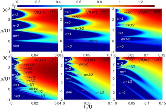
The ground-state phase diagrams of the regular four-chain BH model are shown in figure 7, the ratio β = t_∥/t_⊥ i.e., β = 1 in (a) and β = 0.05 in (b). The existence of the long-range interaction results in the four chains being asymmetrical. Here, we choose the SF order parameter of the first chain to analysis the ground-state phase diagram. Four typical phases are found in a regular four-chain BH model with the long-range interaction, i.e., the SF phase, MI phase, LI phase and SS Phase. When the ratio β = 1, the system only has the SF and MI phases with V/U = 0, which is similar to the phase diagram that in [29]. The MI phases have integer filling atomic numbers per site n = 1, 2, 3, … and the SF phases with nonzero order parameters φ_j1 ≠ 0, as shown in figure 7(a1). By adding the long-range interaction, the SS phases with zero order parameters φ_j1 = 0 are displayed. The SS phase has the half-integer filling per site n = 1/2, 3/2, 5/2, …, which is different the MI phase, one can be seen in figure 7(a(2)). As the long-range interaction is increased to V/U = 3, both the MI phase and the SS phase lobes expand. When the ratio is very small β = 0.05, i.e., t_⊥ ≫ t_∥, the areas of the MI lobes shrink dramatically. Interestingly, there appears a new exotic phase, the LI phase, which has zero order parameter φ and fractional filling atomic number per site n, and the filling atomic number of the LI phase is multiplies of one fourth, i.e., n = p/4, where p = 1, 2, 3, 5, 6, 7, … The LI phases locate the position between the MI phases lobes, as shown in figure 7(b(1)). The LI phases with atomic numbers per site n = p₁/4 (p₁ = 1, 3, 5, 7, …) disappear by considering the long-range interaction. The LI and SS phases with half-integer filling per site are merged together, which make the areas of n = 1/2, 3/2, 5/2, … lobes expand dramatically. As the long-range interaction increases, the phenomenon becomes more obvious, one can be seen in figure 7(b(2))–(b(3)).

Figure 7.

New window|Download| PPT slide
Figure 7.Ground-state phase diagram for the regular four-chain BH model without disorder (Δ = 0) with the on-site interaction U = 1 for the different ratios β = t_∥/t_⊥ i.e., β = 1 in (a) and β = 0.05 in (b). The long-range interaction are V/U = 0, 1 and 3 in a(1)(b(1)), a(2)(b(2)) and a(3)(b(3)), respectively.

5. Summary

We investigated the quantum coherence and ground-state phase transition of a four-chain BH model with the long-range interaction. In a special four-chain BH model, four types of ground-state phases are classified by the atomic number. The effects of the disorder, the on-site interaction and the long-range interaction on the quantum coherence are discussed. When the system without the long-range interaction, with the on-site interaction increasing, the quantum coherence changes from one periodic oscillation to two periodic oscillations. By considering the long-range interaction, the quantum coherence goes back to one periodic oscillation again. The on-site interaction itself suppresses the quantum coherence, both the on-site interaction and long-range interaction together enhance the quantum coherence with the weak disorder, if the disorder strength is increased beyond a critical value, they start to suppress the quantum coherence. In a regular four-chain BH model, the ground-state phase transitions are studied by using the cluster Gutzwiller mean-field method. Exotic ground-state phases, i.e., SF phase, MI phase, SS phase and LI phase are found. When the ratio β = t_∥/t_⊥ is very small, the combination of both the LI and the SS phases expands the lobes with the half-integer filling per site.

Acknowledgments

This work is supported by the NSF of China under Grant No. 11 904 242, the NSF of Hebei province under Grant No. A2019210280.

Reference View Option By original order
By published year
By cited within times
By Impact factor

[1]White M Pasienski M McKay D Zhou S Q Ceperley D DeMarco B 2009 Phys. Rev. Lett. 102 055301
DOI:10.1103/PhysRevLett.102.055301 [Cited within: 1]

[2]Pasienski M McKay D White M DeMarco B 2010 Nature Phys. 6 677
DOI:10.1038/nphys1726

[3]Gadway B Pertot D Reeves J Vogt M Schneble D 2011 Phys. Rev. Lett. 107 145306
DOI:10.1103/PhysRevLett.107.145306

[4]Zhang C Naini A S Sansone B C 2015 Phys. Rev. A 91 031604
DOI:10.1103/PhysRevA.91.031604

[5]Zhang C Sansone B C 2018 Phys. Rev. A 98 013621
DOI:10.1103/PhysRevA.98.013621 [Cited within: 1]

[6]Eisert J van den Worm M Manmana S R Kastner M 2013 Phys. Rev. Lett. 111 260401
DOI:10.1103/PhysRevLett.111.260401 [Cited within: 1]

[7]Jurcevic P Lanyon B P Hauke P Hempel C Zoller P Blatt R Roos C F 2014 Nature (London) 511 202
DOI:10.1038/nature13461

[8]Booth D Rittenhouse S T Yang J Sadeghpour H R Shaffer J P 2015 Science 348 99
DOI:10.1126/science.1260722

[9]Feig M F Gong Z X Clark C W Gorshkov A V 2015 Phys. Rev. Lett. 114 157201
DOI:10.1103/PhysRevLett.114.157201

[10]Cevolani L Carleo G Sanchez-Palencia L 2015 Phys. Rev. A 92 041603(R)
DOI:10.1103/PhysRevA.92.041603 [Cited within: 1]

[11]Kuhner T D Monien H 1998 Phys. Rev. B 58 R14741(R)
DOI:10.1103/PhysRevB.58.R14741 [Cited within: 1]

[12]Kisker J Rieger H 1997 Phys. Rev. B 55 R11981(R)
DOI:10.1103/PhysRevB.55.R11981 [Cited within: 1]

[13]Sengupta P Haas S 2007 Phys. Rev. Lett. 99 050403
DOI:10.1103/PhysRevLett.99.050403

[14]Pollet L Prokofev N V Svistunov B V Troyer M 2009 Phys. Rev. Lett. 103 140402
DOI:10.1103/PhysRevLett.103.140402

[15]Meldgin C et al. 2016 Nature Phys. 12 646 649
DOI:10.1038/nphys3695 [Cited within: 1]

[16]Scarola V W Das Sarma S 2005 Phys. Rev. Lett. 95 033003
DOI:10.1103/PhysRevLett.95.033003 [Cited within: 1]

[17]Bissbort U Thomale R Hofstetter W 2010 Phys. Rev. A 81 063643
DOI:10.1103/PhysRevA.81.063643

[18]Iskin M 2011 Phys. Rev. A 83 051606(R)
DOI:10.1103/PhysRevA.83.051606

[19]Ohgoe T Suzuki T Kawashima N 2012 Phys. Rev. B 86 054520
DOI:10.1103/PhysRevB.86.054520

[20]Deng H M Dai H Huang J H Qin X Z Xu J Zhong H H He C S Lee C H 2015 Phys. Rev. A 92 023618
DOI:10.1103/PhysRevA.92.023618

[21]Xi B Ye F Chen W Q Zhang F C Su G 2011 Phys. Rev. B 84 054512
DOI:10.1103/PhysRevB.84.054512

[22]Ng K K 2015 Phys. Rev. B 91 054516
DOI:10.1103/PhysRevB.91.054516

[23]Kawaki K Kuno Y Ichinose I 2017 Phys. Rev. B 95 195101
DOI:10.1103/PhysRevB.95.195101 [Cited within: 1]

[24]Zhang J M Dong R X 2010 Eur. J. Phys. 31 591 602
DOI:10.1088/0143-0807/31/3/016 [Cited within: 1]

[25]Zhou Q Sarma S D 2010 Phys. Rev. A 82 041601(R)
DOI:10.1103/PhysRevA.82.041601 [Cited within: 2]

[26]Wang J G et al. 2013 J. Phys. B: At. Mol. Opt. Phys. 46 095301
DOI:10.1088/0953-4075/46/9/095301 [Cited within: 2]

[27]Deng H Dai H Huang J Qin X Xu J Zhong H He C Lee C 2015 Phys. Rev. A 92 023618
DOI:10.1103/PhysRevA.92.023618 [Cited within: 1]

[28]Zhang L Qin X Ke Y Lee C 2016 Phys. Rev. A 94 023634
DOI:10.1103/PhysRevA.94.023634 [Cited within: 1]

[29]Fisher M P A Weichman P B Grinstein G Fisher D S 1989 Phys. Rev. B 40 546
DOI:10.1103/PhysRevB.40.546 [Cited within: 1]