Guo-Liang Xu¹, Zi Zhen¹, Yi-Sheng Shi¹, Kang-Xian Guo², E Feddi³, Jian-Hui Yuan^,4, Zhi-Hai Zhang^,1,∗∗1School of Physics and Electronics, Yancheng Teachers University, Yancheng 224002, China
²Department of Physics, College of Physics and Electronic Engineering, Guangzhou University, Guangzhou 510006, China
³Laboratoire de la matière condensée et Sciences Interdisciplinaires (LAMCScI), Group of Optoelectronic of Semiconductors and Nanomaterials, ENSET, Mohammed V University in Rabat, Morocco
⁴Laboratory of Biomedical Photonics and Engineering, Guangxi Medical University, Nanning 530021, China

First author contact: ^∗∗Author to whom any correspondence should be addressed.
Received:2020-12-8Revised:2021-03-11Accepted:2021-03-15Online:2021-07-02

Fund supported:

*Natural Science Foundation of China.11604289 Natural Science Foundation of China.11804063 Natural Science Foundation of China.51971193 BaGui scholar program of Guangxi Province in China and the Natural Science Foundation of Guangxi in China.2016GXNSFBA380017

Abstract
In this study, the effects of hydrostatic pressure and temperature on nonlinear optical rectification (OR), second-harmonic generation (SHG), third-harmonic generation (THG) and the linear, nonlinear, and total optical absorption coefficients (OACs) of a semiparabolic plus semi-inverse squared quantum well (QW) are theoretically investigated. The results show that hydrostatic pressure and temperature have significant effects on the optical properties of semiparabolic plus semi-inverse squared QWs, and that the energy levels and magnitudes of the resonant peaks of OR, SHG, THG, and the total OACs vary according to the shape of the limiting potential, the hydrostatic pressure, and the temperature. It is easily seen that the peak positions of the resonant peaks of OR, SHG, THG, and the total OACs in the semiparabolic plus semi-inverse squared QW show a red shift with increasing hydrostatic pressure, but a blue shift with increasing temperature. Therefore, the magnitude and position of the resonant peaks of OR, SHG, THG, and the total OACs can be adjusted by changing the hydrostatic pressure and the temperature, which promise a new degree of freedom in the tunability of various electro-optical devices.
Keywords： Quantum well;Optical properties;Hydrostatic pressure;Temperature


PDF (1419KB)MetadataMetricsRelated articlesExportEndNote|Ris|BibtexFavorite
Cite this article
Guo-Liang Xu, Zi Zhen, Yi-Sheng Shi, Kang-Xian Guo, E Feddi, Jian-Hui Yuan, Zhi-Hai Zhang. Effects of hydrostatic pressure and temperature on the nonlinear optical properties of semiparabolic plus semi-inverse squared quantum wells^*. Communications in Theoretical Physics, 2021, 73(8): 085502- doi:10.1088/1572-9494/abee70

1. Introduction

In recent years, due to the development of sophisticated growth techniques such as e-beam lithography, reactive ion etching, metal organic chemical vapor deposition and molecular beam epitaxy, the fabrication of artificial low-dimensional semiconductor nanostructures has become feasible [1–4]. Low-dimensional semiconductor nanostructures such as quantum wells (QW), quantum wires, and quantum dots have attracted remarkable attention, from both fundamental and technological points of view. These nanostructures lie between the molecular material and the bulk material. The simultaneous strong quantum confinement of carriers and layering of structures produce not only quantitative but also qualitative differences in physics compared to the the bulk structures, which result in the formation of discrete energy sub-bands that are conducive to drastic changes in the electronic and optical properties. Among these nanostructures, QWs are an integral part of many electronic and optoelectronic devices, because they are easier to grow and fabricate in devices with larger bandgaps and can enhance the strength of electro-optical interactions by confining carriers to small regions. Thus, the optical and electrical properties of these QWs offer a wide range of potential applications in high-performance optical devices such as laser diodes, light-emitting diodes, laser amplifiers, photo-detectors, high-speed electro-optical modulators, and so on [5–7].

In the study of low-dimensional systems, one of the most interesting properties to explore is the influence of spatial confinement on the energy spectra and nonlinear optical properties of a QW system. Most experimental and theoretical investigations have examined the effects of the shape, size, and confining potential in QW systems, which have provided great advantages in terms of tuning the desired optical properties. Chen et al theoretically studied nonlinear optical rectification (OR) in double triangular QWs. The results showed that the theoretical value of OR was 2 − 3 orders of magnitude higher that in a single QW system [8]. H. Hassanabadi et al reported nonlinear OR and second-harmonic generation (SHG) in semiparabolic and semi-inverse squared QWs, and confirmed that the magnitudes of both the OR coefficients and the SHG susceptibility decreased and increased with an increase in the confinement frequency Ω₀ and the geometric structural parameter β [9]. S. Şakiroğlu et al reported OR, SHG, and third-harmonic generation (THG) in a Pöschl-Teller QW. The results showed that the peak positions were sensitive to the asymmetry parameters governing the confinement potential, and that the nonlinear OR and SHG susceptibility increased with an enhancement in the asymmetry of the QW; they also showed that the maximum asymmetry was be obtained using an optimized set of parameters [10]. Z.M. Zhang et al studied the THG susceptibilities, the nonlinear optical absorption coefficients (OACs) and the refractive index changes (RICs) of a square tangent QW and confirmed that the THG susceptibilities, the OACs and the RICs were strongly affected by d and U₀, which had great influence on the geometry of the QW [11]. Consequently, the geometric structure factor greatly affects the electrical, optical, and transport behavior of QW systems.

Recently, investigation of the nonlinear optical properties of QWs together with various physical effects, such as hydrostatic pressure, temperature, external electric, and magnetic fields, and so on, has been the topic of many theoretical and experimental studies, which have realized the effective adjustment of nonlinear optical properties. J.H. Yuan et al studied the effects of applied electric fields on the SHG in semiparabolic QWs. Their results indicated that an increase in the applied electric field can weaken the peak values of SHG, but that the nonlinear OR was strengthened [12]. The influences of the applied magnetic field, temperature, and hydrostatic pressure on the nonlinear optical properties of a symmetric double semi-V-shaped QW were studied by U. Yesilgul et al [13]. S. Şakiroğlu calculated the linear and nonlinear OACs and RICs of Morse QWs under the influence of a static electric field [14]. X. Liu et al reported the nonlinear OR and SHG in asymmetrical Gaussian QWs under the influence of applied magnetic fields, temperatures, and hydrostatic pressures [15]. The nonlinear OR and SHG in a semiparabolic QW under the influence of an intense laser field along with applied electric and magnetic fields were theoretically studied by F. Ungan et al [16]. S. Şakiroğlu et al reported the effects of an intense laser field and an applied electric field on the nonlinear OACs and RICs in a Morse QW [17]. According to these reports, it was found that not only the structural parameters but also the external physical fields have great influence on the optical characteristics of these structures. Such a system can be used to control and adjust the density output of semiconductor devices, which also provide the desired optical properties for device outlines.

The purpose of this work is to investigate the effects of hydrostatic pressure and temperature on the nonlinear optical properties of a semiparabolic plus semi-inverse squared QW, which have not yet been discussed. This paper is organized as follows: section 2 contains the details of the theoretical framework. The results and a discussion are presented in section 3. Finally, the conclusions are given in section 4.

2. Theory

In the framework of effective mass approximation, the Hamiltonian for GaAs/Al_xGa_1−x As semiparabolic plus semi-inverse squared QWs under the influence of hydrostatic pressure P and temperature T may be written as:(1)$\begin{eqnarray}H=-\displaystyle \frac{{{\hslash }}^{2}}{2{m}^{* }(P,T)}{{\rm{\nabla }}}_{z}^{2}+V(z,P,T).\end{eqnarray}$

Here, m^*(P, T) = (0.0665 + 0.0835x), m^*(P, T) is the hydrostatic pressure- (P) and temperature- (T) dependent electron effective mass, the aluminum concentration is given by x = 0.3, while for GaAs m^*(z) = 0.067m₀ (m₀ is the free electron mass), and V(z, P, T) is the semiparabolic plus semi-inverse squared confining potential. They are given by [13, 15, 18, 19](2)$\begin{eqnarray}\begin{array}{rcl}{m}^{* }(P,T) & = & {m}_{0}\left[1\right.\\ & & {\left.+\{{E}_{P}^{{\rm{\Gamma }}}\left\{\displaystyle \frac{2}{{E}_{g}^{{\rm{\Gamma }}}(P,T)}+\displaystyle \frac{1}{{E}_{g}^{{\rm{\Gamma }}}(P,T)+{{\rm{\Delta }}}_{0}}\right\}\right]}^{-1},\end{array}\end{eqnarray}$where Δ₀ = 0.341 eV is the spin-orbit split of the valence band for GaAs. ${E}_{P}^{{\rm{\Gamma }}}=7.51\,\mathrm{eV}$ is the energy related to the momentum matrix element. ${E}_{g}^{{\rm{\Gamma }}}(P,T)={E}_{g}^{{\rm{\Gamma }}}(0,T)\,+{bP}+{{cP}}^{2}$ is the variation of the energy gap at the Γ − point for a GaAs semiconductor with hydrostatic pressure P and temperature T, as follows: ${E}_{g}^{{\rm{\Gamma }}}(0,T)=[1.519-(5.405\times {10}^{-4}{T}^{2})/(T+204)]$ eV, b = 1.26 × 10⁻² eV/bar and c = − 3.77 × 10⁻⁵ eV/kbar².

The semiparabolic plus semi-inverse squared confining potential is given by(3)$\begin{eqnarray}V(z,P,T)=\left\{\begin{array}{ll}\tfrac{1}{2}{m}^{* }(P,T){\omega }_{z}^{2}{z}^{2}+\tfrac{{{\hslash }}^{2}\beta }{2{m}^{* }(P,T){z}^{2}} & 0\leqslant z\lt {L}_{P}\\ \infty & z\lt 0,\end{array}\right.\end{eqnarray}$where Ω_z and β are the confinement frequency and the characteristic parameter of the inverse squared potential, respectively, which control the asymmetry degree of the potential well. Also, L_P is the pressure-dependent characteristic size of the QW, which is obtained from the fractional change in the volume of the sample: L_P = L[1 − (1.16 × 10⁻³ kbar⁻¹ − 7.4 × 10⁻⁴ kbar⁻¹)P], where L is the original width of the confinement potentials in the z direction.

In this manuscript, we use the finite difference technique to obtain the numerical solution of the Schrödinger equation (1) after the energies and the corresponding envelope wave functions have been obtained. The nonlinear optical properties for OR ${\chi }_{0}^{(2)}$, SHG ${\chi }_{2\omega }^{(2)}$, THG ${\chi }_{3\omega }^{(3)}$ and the OACs α(Ω,I) can be easily calculated using the compact density matrix method and the iterative procedure, which are given by [18–22](4)$\begin{eqnarray}\begin{array}{l}{\chi }_{0}^{(2)}=\displaystyle \frac{4{e}^{3}{\sigma }_{\nu }}{{\varepsilon }_{0}{{\hslash }}^{2}}{\mu }_{10}{\delta }_{10}\\ \ \ \times \,\displaystyle \frac{{E}_{10}^{2}(1+\tfrac{{{\rm{\Gamma }}}_{2}}{{{\rm{\Gamma }}}_{1}})+({\left({\hslash }\omega \right)}^{2}+{\left(\tfrac{{\hslash }}{{T}_{2}}\right)}^{2})(\tfrac{{{\rm{\Gamma }}}_{2}}{{{\rm{\Gamma }}}_{1}}-1)}{\left[{\left({E}_{10}-{\hslash }\omega \right)}^{2}+{{\rm{\Gamma }}}_{2}^{2}][{\left({E}_{10}+{\hslash }\omega \right)}^{2}+{\left(\tfrac{{\hslash }}{{T}_{2}}\right)}^{2}\right]},\end{array}\end{eqnarray}$(5)$\begin{eqnarray}{\chi }_{2\omega }^{(2)}=\displaystyle \frac{{e}^{3}{\sigma }_{\nu }}{{\varepsilon }_{0}}\displaystyle \frac{{\mu }_{01}{\mu }_{12}{\mu }_{20}}{({\hslash }\omega -{E}_{10}-{\rm{i}}{\hslash }{{\rm{\Gamma }}}_{0})(2{\hslash }\omega -{E}_{20}-{\rm{i}}{\hslash }{{\rm{\Gamma }}}_{0})},\end{eqnarray}$(6)$\begin{eqnarray}\begin{array}{l}{\chi }_{3\omega }^{(3)}\\ =\,\displaystyle \frac{{e}^{4}{\sigma }_{\nu }}{{\varepsilon }_{0}}\displaystyle \frac{{\mu }_{01}{\mu }_{12}{\mu }_{23}{\mu }_{30}}{({\hslash }\omega -{E}_{10}-{\rm{i}}{\hslash }{{\rm{\Gamma }}}_{12})(2{\hslash }\omega -{E}_{20}-{\rm{i}}{\hslash }{{\rm{\Gamma }}}_{12})(3{\hslash }\omega -{E}_{30}-{\rm{i}}{\hslash }{{\rm{\Gamma }}}_{12})}.\end{array}\end{eqnarray}$

The analytical forms of the linear and third-order nonlinear OACs are then given by(7)$\begin{eqnarray}{\alpha }^{(1)}(\omega )=\omega \sqrt{\displaystyle \frac{\mu }{{\varepsilon }_{{\rm{R}}}}}\displaystyle \frac{| {\mu }_{10}{| }^{2}{\sigma }_{\nu }{\hslash }{{\rm{\Gamma }}}_{23}}{{\left({E}_{10}-{\hslash }\omega \right)}^{2}+{\left({\hslash }{{\rm{\Gamma }}}_{23}\right)}^{2}},\end{eqnarray}$(8)$\begin{eqnarray}\begin{array}{rcl}{\alpha }^{(3)}(\omega ,I) & = & \omega \sqrt{\displaystyle \frac{\mu }{{\varepsilon }_{{\rm{R}}}}}\left(\displaystyle \frac{I}{2{\varepsilon }_{0}{n}_{{\rm{r}}}c}\right)\\ & & \times \,\displaystyle \frac{| {\mu }_{10}{| }^{2}{\sigma }_{\nu }{\hslash }{{\rm{\Gamma }}}_{23}}{{\left[{\left({E}_{10}-{\hslash }\omega \right)}^{2}+{\left({\hslash }{{\rm{\Gamma }}}_{23}\right)}^{2}\right]}^{2}}[4| {\mu }_{10}{| }^{2}\\ & & -\,\displaystyle \frac{| {\mu }_{11}-{\mu }_{00}{| }^{2}[3{E}_{10}^{2}-4{E}_{10}{\hslash }\omega +{{\hslash }}^{2}({\omega }^{2}-{{\rm{\Gamma }}}_{23}^{2})]}{{E}_{10}^{2}+{\left({\hslash }{{\rm{\Gamma }}}_{23}\right)}^{2}}].\end{array}\end{eqnarray}$

Therefore, the total absorption coefficient α(Ω,I) is given by(9)$\begin{eqnarray}\alpha (\omega ,I)={\alpha }^{(1)}(\omega )+{\alpha }^{(3)}(\omega ),\end{eqnarray}$where Σ_ν is the density of electrons in the QW, μ_ij = ∣⟨ψ_i∣z∣ψ_j⟩∣ (i, j = 0, 1, 2, 3) is the off-diagonal matrix element, δ₀₁ = ∣μ₁₁ − μ₀₀∣, Ω₀₁ is the transition frequency, μ is the permeability of the system, E_ij = E_i − E_j is the energy interval between two different electronic states, I is the incident optical intensity, and Γ_k = 1/T_k with k = (0, 1, 2, 3) are damping terms associated with the lifetime of the electrons involved in the transitions.

3. Results and discussion

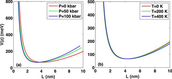
In the numerical calculations for the Al_xGa_1−x As/GaAs semiparabolic plus semi-inverse squared QW, the following material parameters are used [21–24]: L = 10nm, n_r = 3.2, ϵ₀ = 8.85 × 10⁻¹² Fm⁻¹, ${\varepsilon }_{R}={n}_{r}^{2}{\varepsilon }_{0}$, T₀ = 0.14 ps, T₁ = 1 ps, T₂ = 0.2 ps, T₁₂ = 0.5 ps, T₂₃ = 0.12 ps, I = 1 × 10¹⁰ MW/cm², Γ₁₂ = 1/T₁₂, and Σ_ν = 5 × 10²⁴ m⁻³.

Initially, in order to show the effects of hydrostatic pressure P and temperature T on the confining potential, in figure 1(a) we present the variation of the potential shape for three different values of hydrostatic pressure, P = 0, P = 50 kbar, and P = 100 kbar. It is clear from the figure that the well width decreases slightly with increasing hydrostatic pressure P, which leads to stronger confinement of the carriers, causing an enhancement of the energy differences E₁₀, E₂₀, and E₃₀. In figure 1(b) we present the variation of the potential shape for three different temperature values, T = 0, T = 200 K, T = 400 K, and find that the well width and well depth change very little as the temperature T increases. Therefore, the effect of temperature T on the confined potential is negligible.

Figure 1.

New window|Download| PPT slide
Figure 1.Pictorial view of the confinement potential in a semiparabolic plus semi-inverse squared QW for two different variables: (a) hydrostatic pressure P and (b) temperature T.


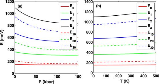
Figures 2(a) and (b) show the variation of the energy eigenvalues E₀, E₁, E₂, and E₃ and the energy differences E₁₀, E₂₀, and E₃₀ as a function of the hydrostatic pressure P and the temperature T with T = 0 and P = 0, respectively. As can be seen from figure 2(a), as the hydrostatic pressure P increases, the values of the conduction energy levels E₀, E₁, E₂, and E₃ decrease monotonically. Moreover, the higher the energy level, the more sensitive the QW is to the variation of hydrostatic pressure P. This is the case because when the hydrostatic pressure P increases, the electron’s effective mass increases. Obviously, the influence of the hydrostatic pressure P on the effective mass is more dominant than that of the confined potential, which causes a reduction of the values of the conduction energy levels. Therefore, we can easily see that the energy differences E₁₀, E₂₀, and E₃₀ decrease when the hydrostatic pressure P increases. From figure 2(b), it can be seen that, as the temperature T increases, the values of the conduction energy levels E₀, E₁, E₂, and E₃ increase. This is because the structural parameters such as the electron’s effective mass and the conduction band offset decrease with increasing temperature T. Moreover, the energy levels of the excited states change more obviously with temperature T, and the ground state increases a little with an increase in the temperature T. For this reason, the energy differences between the first excited state and the ground E₁₀, the second excited state and the ground E₂₀ and the third excited state and the ground E₃₀ of the system increase as the temperature T increases.

Figure 2.

New window|Download| PPT slide
Figure 2.The energy eigenvalues E₀, E₁, E₂, and E₃ and energy differences E₁₀, E₂₀, and E₃₀ are plotted as a function of the (a) hydrostatic pressure P and (b) the temperature T, respectively.


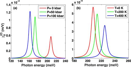
In figure 3, we can observe the behavior of the nonlinear OR ${\chi }_{0}^{(2)}$, calculated as a function of the photon energy. Several distinct values of (a) hydrostatic pressure (P = 0, 50 kbar, 100 kbar) with T = 0 K, and (b) temperature (T = 0, 200 K, 400 K) with P = 0 kbar have been discussed, respectively. As can be seen from figure 3(a), the following points can be deduced: (1) the nonlinear OR ${\chi }_{0}^{(2)}$ coefficient has a maximum (in any curve and for different hydrostatic pressures P) at a photon energy equal to the energy difference between the ground state and the first excited state E₁₀, which is the resonant photon energy; (2) the amplitude of the resonant peak of nonlinear OR ${\chi }_{0}^{(2)}$ increases with increasing hydrostatic pressure P. The physical reason for this behavior is that when the hydrostatic pressure P increases, the transition matrix element μ₁₀ increases because the electron’s effective mass and the conduction band offset increase with increasing P. Also, the positions of the resonant peaks shift toward lower energies (a red shift), because the energy difference E₁₀ decreases with increasing hydrostatic pressure P. This behavior is in agreement with figure 2(a). It can be seen from figure 3(b) that the amplitude of the resonant peak of nonlinear OR ${\chi }_{0}^{(2)}$ is directly related to the temperature T and decreases with an increase in the temperature T. The physical reason for this is a reduction of transition matrix element μ₁₀ because the electron’s effective mass and the conduction band offset decrease with an increase in temperature T. For this reason, the energy difference E₁₀ between the first excited state and the ground state of the system increases. Therefore, as the temperature T increases, the resonant peak positions of nonlinear OR shift toward higher energies.

Figure 3.

New window|Download| PPT slide
Figure 3.The variation of nonlinear OR ${\chi }_{0}^{(2)}$ as a function of the photon energy for different hydrostatic pressures P (a), and temperatures T (b), respectively.


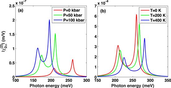
Figure 4 shows the variations of the SHG ${\chi }_{2\omega }^{(2)}$ as a function of photon energy for three different values of hydrostatic pressure P = 0, P = 50 kbar, and P = 100 kbar (a) and temperature T = 0, T = 200 K, T = 400 K (b), respectively. From figure 4(a), it can be seen that the SHG ${\chi }_{2\omega }^{(2)}$ susceptibility has two resonant peaks (in any curve and for different hydrostatic pressures P), where the photon energy is equal to the energy difference between the ground state and the first excited state E₁₀ and the energy difference between the ground state and the second excited state E₂₀, which is the resonant photon energy. Meanwhile, the locations of the resonant peaks of SHG ${\chi }_{2\omega }^{(2)}$ shift toward lower energies with increasing hydrostatic pressure P. Also, the amplitudes of the resonant peaks of SHG ${\chi }_{2\omega }^{(2)}$ increase when the hydrostatic pressure P increases. The physical origin of this behavior is that the electron’s effective mass and the quantum confinement effect increase. When the electron’s effective mass changes, the energy differences E₁₀ and E₂₀ and the overlaps of state also change. It can be seen from figure 4(b) that the resonant peak positions of SHG ${\chi }_{2\omega }^{(2)}$ move to higher energy regions when the temperature T increases. Also, the amplitudes of the resonant peaks of SHG ${\chi }_{2\omega }^{(2)}$ decrease with increasing temperature T. The physical origin of this behavior is the decrease of the electron’s effective mass and the conduction band offset when the temperature T increases. When the electron’s effective mass changes, the energy differences E₁₀ and E₂₀ and the overlaps of state also change. This is true with the exception of the cases depicted in figures 2(a) and (b).

Figure 4.

New window|Download| PPT slide
Figure 4.The variation of SHG ${\chi }_{2\omega }^{(2)}$ as a function of photon energy for three different values of hydrostatic pressure P (a) and temperature T (b), respectively.


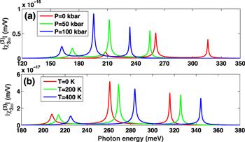
The effects of hydrostatic pressure P and temperature T on the THG ${\chi }_{3\omega }^{(3)}$ are plotted in figures 5(a) and (b), respectively. As can be seen from these figures, the following points can be deduced: (1) three different resonant peaks are seen in the THG ${\chi }_{3\omega }^{(3)}$ spectrum, corresponding to one-photon resonance(E₁₀ = ℏΩ), two-photon resonance(E₂₀ = 2ℏΩ), and three-photon resonance(E₃₀ = 3ℏΩ); (2) an increase in the hydrostatic pressure P results in a red shift of the THG ${\chi }_{3\omega }^{(3)}$ spectrum. This is due to a decrease in the energy differences E₁₀, E₂₀, and E₃₀ (as shown in figure 2(a)). Also, the magnitudes of all resonant peaks increase with increasing hydrostatic pressure P, which illustrates the complex competitive coupling mechanisms caused by hydrostatic pressure P; (3) the larger the temperature T, the smaller the value of THG ${\chi }_{3\omega }^{(3)}$. The physical reason for this feature is that the electron’s effective mass and the overlaps between different electronic states reduce with increasing temperature T. Also, the positions of the resonant peaks of THG ${\chi }_{3\omega }^{(3)}$ display a blue shift when the temperature T increases. This is because the energy intervals E₁₀, E₂₀, and E₃₀ increase with an increase of the temperature T, which related to the fact that the electron’s effective mass and the conduction band offset decrease with temperature T (as shown in figure 2(b)).

Figure 5.

New window|Download| PPT slide
Figure 5.The variation of THG ${\chi }_{3\omega }^{(3)}$ as a function of the photon energy for three different values of hydrostatic pressure P(a) and temperature T(b), respectively.


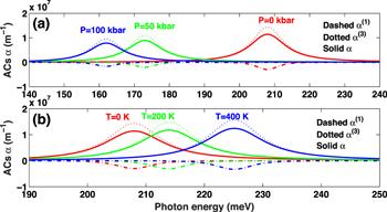
In figure 6, the linear α⁽¹⁾, nonlinear α⁽³⁾, and total OACs α are plotted as a function of the incident photon energy for three different values of hydrostatic pressure P = 0, P = 50 kbar, P = 100 kbar and temperatures T = 0, T = 200 K, T = 400 K, respectively. As can be seen in figure 6(a), the total OAC α is significantly reduced due to a nonlinear contribution with increasing hydrostatic pressure P, and the nonlinearity of α⁽³⁾ should be considered when the intensity of the incoming radiation is strong enough, which leads to a reduction in the total absorption. In addition, the corresponding peak positions of the linear α⁽¹⁾, nonlinear α⁽³⁾, and total OACs α undergo a red shift. This is because the electron’s effective mass increases with increasing hydrostatic pressure P, which reflects the competitive relationship between the kinetic and potential energies of the system(see figure 2(a)). From figure 6(b), we can see that, as an immediate effect of augmenting the magnitude of the temperature T, the amplitudes of the resonant peaks of the total OACs α present an increase in their heights or intensities. Also, the most notable effect is an obvious blue shift of the positions of the resonant peaks of the total OACs α with increasing temperature T. This shift is caused by the increased energy level distance when the temperature T changes(see figure 2(b)).

Figure 6.

New window|Download| PPT slide
Figure 6.The variation of the linear α⁽¹⁾, nonlinear α⁽³⁾, and total OACs α as a function of the photon energy for three different values of hydrostatic pressure P (a) and temperature T (b), respectively.

4. Conclusions

In this work, we have investigated the effects of hydrostatic pressure P and temperature T on the nonlinear OR ${\chi }_{0}^{(2)}$, SHG ${\chi }_{2\omega }^{(2)}$, THG ${\chi }_{3\omega }^{(3)}$ and total OACs α of a semiparabolic plus semi-inverse squared QW using the finite difference method. The optical properties calculated within the framework of the compact density matrix approach and an iterative scheme were investigated for varying strengths of the hydrostatic pressure P and the temperature T. The numerical results revealed that an adjustment of the hydrostatic pressure P and the temperature T that govern the confining potential and the electron effective’s mass can lead to a change in the optical response of the system. However, the change to the electron’s effective mass caused by the hydrostatic pressure P and the temperature T plays an important role in the optical response of the system. Moreover, as the hydrostatic pressure P increases, the amplitudes of the resonant peaks of nonlinear OR ${\chi }_{0}^{(2)}$, SHG ${\chi }_{2\omega }^{(2)}$ and THG ${\chi }_{3\omega }^{(3)}$ increase significantly. However, the amplitudes of the resonant peaks of the total OACs, α, changed inversely. In addition, a red shift in the peaks was obtained. With increasing temperature T, the resonant peaks of the nonlinear OR ${\chi }_{0}^{(2)}$, SHG ${\chi }_{2\omega }^{(2)}$ and THG ${\chi }_{3\omega }^{(3)}$ experience an obvious blue shift, and the amplitudes of the resonant peaks of nonlinear OR ${\chi }_{0}^{(2)}$, SHG ${\chi }_{2\omega }^{(2)}$ and THG ${\chi }_{3\omega }^{(3)}$ decrease significantly, which is contrary to the change of amplitude of the resonant peaks of the total OACs, α. We conclude that the hydrostatic pressure and temperature may serve as a probe for the controllability of the nonlinear optical properties of the QW.

Reference View Option By original order
By published year
By cited within times
By Impact factor

[1]Cho A Y Arhur J R 1975 Prog. Solid State Chem. 10 157
DOI:10.1016/0079-6786(75)90005-9 [Cited within: 1]

[2]Sundaram M Chalmers S A Hopkins P E Gossard A C 1991 Science 254 1326
DOI:10.1126/science.254.5036.1326

[3]Panish M R 1980 Science 208 916
DOI:10.1126/science.208.4446.916

[4]Sirtori C Capasso F Sivco D L Cho A Y 1992 Phys. Rev. Lett. 68 1010
DOI:10.1103/PhysRevLett.68.1010 [Cited within: 1]

[5]Lei W Chen Y H Wang Y L Huang X Q Ch Zhao Liu J Q Xu B Jin P Zeng Y P Wang Z G 2006 J. Crystal Growth 286 23
DOI:10.1016/j.jcrysgro.2005.09.054 [Cited within: 1]

[6]Khordad R Mirhosseini B 2014 Opt. Spectrosc. 117 434
DOI:10.1134/S0030400X14090100

[7]Arunachalam N John Peter A Lee C W 2011 Phydica E 44 590 596
DOI:10.1016/j.physe.2011.10.009 [Cited within: 1]

[8]Chen B Guo K X Wang R Z Zhang Z H Liu Z L 2009 Solid State Commun. 149 310 314
DOI:10.1016/j.ssc.2008.11.032 [Cited within: 1]

[9]Hassanabadi H Liu G H Lu L L 2012 Solid State Commun. 152 1761 1766
DOI:10.1016/j.ssc.2012.05.023 [Cited within: 1]

[10]Şakiroglu S Ungan F Yesilgul U Mora-Ramos M E Duque C A Kasapoglu E Sari H Sökmen I 2012 Phys. Lett. A 376 1875 1880
DOI:10.1016/j.physleta.2012.04.028 [Cited within: 1]

[11]Zhang Z M Guo K X Mou S Xiao B Zhou Y C 2016 Optik 127 928 933
DOI:10.1016/j.ijleo.2015.10.125 [Cited within: 1]

[12]Yuan J H Chen N Zhang Y Mo H Zhang Z H 2016 Physica E 77 102 107
DOI:10.1016/j.physe.2015.11.011 [Cited within: 1]

[13]Yesilgul U Ungan F Al E B Kasapoglu E Sari H Sökmen I 2016 Opt. Quant. Electron 48 560
DOI:10.1007/s11082-016-0838-x [Cited within: 2]

[14]Sakiroglu S 2016 Int. J. Mod. Phys. B 30 1650209
DOI:10.1142/S021797921650209X [Cited within: 1]

[15]Liu X Zou L L Liu C L Zhang Z H Yuan J H 2016 Opt. Mater. 53 218 223
DOI:10.1016/j.optmat.2016.01.043 [Cited within: 2]

[16]Ungan F Martinez-Orozco J C Restrepo R L Mora-Ramos M E Kasapoglu E Duque C A 2015 Superlatt. and Microstruct 81 26 33
DOI:10.1016/j.spmi.2015.01.016 [Cited within: 1]

[17]Sakiroglu S Kasapoglu E Restrepo R L Duque C A Sökmen I 2017 Phys. Status Dolid B 254 1600457
DOI:10.1002/pssb.201600457 [Cited within: 1]

[18]Emine O Ismail S 2012 Opt. Commun. 285 5223 5228
DOI:10.1016/j.optcom.2012.08.001 [Cited within: 2]

[19]Zhang Z H Yuan J H Guo K X 2018 Materials 11 668
DOI:10.3390/ma11050668 [Cited within: 1]

[20]Zhang Z H Yuan J H Guo K X Feddi E 2019 Materials 12 78
DOI:10.3390/ma12010078

[21]Zhang Z H Zou L L Guo K X Yuan J H 2016 Opt. Commun. 359 316 321
DOI:10.1016/j.optcom.2015.10.015 [Cited within: 1]

[22]Hu L Guo K X Zhang Z M Jiang X C Li K Y Liu D F 2017 Int. J. Mod. Phys. B 31 1750009
DOI:10.1142/S0217979217500096 [Cited within: 1]

[23]Keshavarz A Zamani N 2013 Superlatt. and Microstruct. 58 191 197
DOI:10.1016/j.spmi.2013.03.014

[24]Zhang Z H Guo K X Yuan J H 2019 Physica E 108 238 243
DOI:10.1016/j.physe.2018.12.034 [Cited within: 1]