<script type="text/javascript" src="https://cdn.bootcss.com/mathjax/2.7.2-beta.0/MathJax.js?config=TeX-AMS-MML_HTMLorMML"></script> <script type='text/x-mathjax-config'> MathJax.Hub.Config({ extensions: ["tex2jax.js"], jax: ["input/TeX", "output/HTML-CSS"], tex2jax: {inlineMath: [ ['$','$'], ["\\(","\\)"] ],displayMath: [ ['$$','$$'], ["\\[","\\]"] ],processEscapes: true}, "HTML-CSS": { availableFonts: ["TeX"] }, "HTML-CSS": {linebreaks: {automatic: true}}, SVG: {linebreaks: {automatic: true}} }); </script> Najeeb Alam Khan^,1, Muhammad Ali Qureshi², Tooba Hameed¹, Saeed Akbar¹, Saif Ullah³¹Department of Mathematics, University of Karachi, Karachi 75270, Pakistan
²Department of Physics, University of Karachi, Karachi 75270, Pakistan
³Department of Mathematics, Government College University, Lahore 54000, Pakistan

Received:2020-04-22Revised:2020-08-04Accepted:2020-08-04Online:2020-11-12


Abstract
In this paper, we propose an innovative chaotic system, combining fractional derivative and sine-hyperbolic nonlinearity with circuit execution. The study of this system is conducted via an analog circuit simulator, using two anti-parallel semiconductor diodes to provide hyperbolic sine nonlinearity, and to function as operational amplifiers. The multi-stability of the system is also enhanced with the help of multi-equilibrium points for distinct real orders of system. The system explores the generation of a four-wing attractor in different phases, both numerically and electronically. By changing the input parameters of the system, different graphs are generated for current flow in state, phase, and space, to confirm the precision of the fractional order derivatives. A reasonable simulation shows that the deliberate circuit provides effective chaos in terms of speed and accuracy, which is comensurate with the numerical simulation. This nonlinear chaotic behavior is utilized to encrypt sound (.wav), images (.jpg), and animated (.gif) data which are a major requirement for the security of communication systems. The proposed circuit performs chaos and cryptographic tasks with high-effective analog computation, and constitutes a novel approach to this area of research.
Keywords： multi-wing attractors;hyperbolic sine;circuit realization;encryption


PDF (5434KB)MetadataMetricsRelated articlesExportEndNote|Ris|BibtexFavorite
Cite this article
Najeeb Alam Khan, Muhammad Ali Qureshi, Tooba Hameed, Saeed Akbar, Saif Ullah. Behavioral effects of a four-wing attractor with circuit realization: a cryptographic perspective on immersion. Communications in Theoretical Physics, 2020, 72(12): 125004- doi:10.1088/1572-9494/abb7d1

1. Introduction

The modern era has seen many great contributions, both theoretical and experimental, on the subject of fractional calculus, with its long history of non-integer order [1]. Some well-known types of fractional derivatives (FDs) include those proposed by Liouville, Riezs, Riemann, Caputo, Letnikov, Hadamard, Marchaud, Weyl, and Coimbra, among others. The role of FDs in science is to store information about a system's temporal and spatial non-locality, where non-locality is useful for describing an object's instant state variation spatially; with respect to time, this is known as memory [2]. The key representative property claimed for the FD is that it violates the standard Leibniz rule [3]; this property, while necessary, is not sufficient. The standard Leibniz rule is violated by various integro-differential operators, but it is important to note that these are not derivatives of a non-integer order. As mentioned above, spatial and temporal non-locality are new tools for defining systems, and the process is considered to be one of the most significant properties of FDs. The property of non-locality, in mathematical terms, states that a FD cannot be embodied as a finite set of derivatives of integer orders. Thus, based on the non-locality principle, we cannot describe non-local systems and processes containing differential equations only in terms of the derivatives of integer order [4].

The chaotic system is an initial condition-sensitive and nonlinear dynamical system which is affected even by small variations, and was first introduced by Lorenz in 1963 in the context of a study of weather models, which constitute a two-scroll chaotic attractor [5]. After Lorenz's discovery of the chaotic system, the theory has been utilized in many different fields of science, including physics [6, 7], reactors [8], memristors [9], and encryption [10]. Chaotic attractors are classified into two categories: (i) self-excited attractors, and (ii) hidden attractors. Self-excited attractors possess a basin of attraction, created by to the intersection of unstable equilibrium points, and hidden attractors do not intersect with the neighborhood of equilibrium points.

In engineering applications, more complicated topological nonlinear periodic [11, 12] and chaotic [13] systems are widely employed in systems such as multi-wing attractors or multi-scrolls [14, 15]. For scientists, they therefore represent an attractive field of research. Multi-scroll systems can basically be categorized into into two types: the generalization of Chua's circuit [16], and the generalization of the Lorenz circuit [17]. The autonomous four-wing butterfly was proposed by Elwakil [18] having both symmetrical and non-symmetrical versions. Zidan et al then proposed a new V-shaped multi-scroll attractor [19]. Zhang [20] proposed a four-dimensional hyperchaotic system by modifying Lu's double-wing hyperchaotic system. Based on the saw tooth wave function, the Lorentz system was modified by Simin et al for generating multi-wing butterfly chaotic attractors [21]. Utilizing Lu's system, a new piece-wise linear function was considered, in order to generate a multi-wing butterfly chaotic system. The four-wing system achieved by Wang [22] was derived from previous 3D four-wing smooth continuous chaotic systems [23], and enhanced by extending these chaotic systems by adding linear or quadratic terms to the system. Research is ongoing in relation to methodology, theory, and application in multi-wing chaotic system, and great progress is being made [24]. Recently, Wang and Volos [25] initiated a simple three-dimensional system, and discussed the special features required for system validation. In this work, we extend Wang's model by taking the memory term via the time fractional derivative in the following form:(1)$\begin{eqnarray}\begin{array}{c}\begin{array}{l}{{\rm{D}}}_{t}^{\alpha }{u}_{1}\left(t\right)=-a{u}_{1}\left(t\right)+{u}_{2}\left(t\right){u}_{3}\left(t\right),\\ {{\rm{D}}}_{t}^{\alpha }{u}_{2}\left(t\right)=-\,\sinh \left({u}_{2}\left(t\right)\right)+{u}_{1}\left(t\right){u}_{3}\left(t\right),\\ {{\rm{D}}}_{t}^{\alpha }{u}_{3}\left(t\right)={u}_{3}\left(t\right)-{u}_{1}\left(t\right){u}_{2}\left(t\right),\\ 0\lt \alpha \leqslant 1,\,0\leqslant t\leqslant T,\end{array}\end{array}\end{eqnarray}$with initial conditions(2)$\begin{eqnarray}{u}_{1}\left(0\right)=0.1,{u}_{2}\left(0\right)=0.1,{u}_{3}\left(0\right)=0.1.\end{eqnarray}$Here, $\alpha $ is the order of the fractional derivative, $a$ denotes any positive parameter, and ${u}_{1},{u}_{2},{u}_{3}$ are state variables of the system. The system (1)-(2) is a four-term novel chaotic system, with one hyperbolic sine and three quadratic nonlinearities. Wang also observed the behavioral effects of systems (1) for distinct values of $a$ in system (1) at $\alpha =1,$, which displays chaotic behavior with limit cycles and a multi-wing attractor. The multi-wing attractor, along with the fractional derivative, is a more complex system, and is sensitive to the parameters and initial conditions of a system, giving rise to various potential applications in the field of secure communication.

The public network of communication systems has rapidly become digitized over the past few years, as cross-country communication issues, such as transportation problems, speed of communication, confidentiality, etc, have arisen. The intelligence community is familiar with these issues, and protects our information using different mathematical methods, such as stenography and cryptography. Cryptography is an art among sciences, in that it creates meaningless redundancy around sensitive data as random entropy increases, so that data compression becomes more difficult for the would-be infiltrator. The multi-wing attractor, along with the fractional order mathematical system scheme, represents the process of evolution in the field of cryptography, in terms of the generation of random numbers, tested with NIST-800-22, and of complicated encryption processes, driven by a need for the secure communication of sensitive data.

The aim of this work is to present a multi-wing attractor using sine-hyperbolic nonlinearity combined with fractional order. The mathematical model, and other dynamic parameters, are calculated, and discussed in detail in the following sections, along with the electronic realization simulated in MultiSIM for different values of fractional order, using passive components such as Resistors, Capacitors, and Diodes, and active components, i.e. operational amplifiers. We conclude by investigating the cryptographic capability of our multi-wing chaotic system, using the Python programming language, to perform encryption for voice, image, and animation image data for cellular and telecommunication applications.

2. Preliminary definitions

In this section, the preliminary definitions used in this paper as tools for guidance, together with their properties, are elucidated.

Definition 2.1. The Caputo derivative

Assume $\theta \left(t\right)$ to be a continuous function ($\theta \left(t\right)\,\in {C}^{m}\left[0,1\right]$); the FD, in the Caputo sense of $\theta \left(t\right)$, with respect to $t$, is then defined as [1]:(3)$\begin{eqnarray}\begin{array}{l}{{\rm{D}}}^{\alpha }\theta \left(t\right)=\left\{\begin{array}{cc}{I}_{t}^{q-\alpha }{{\rm{D}}}^{m}\theta \left(t\right), & q-1\lt \alpha \leqslant q\\ {{\rm{D}}}^{q}\theta \left(t\right), & \alpha =q\in N\end{array}\right.,\\ \,\alpha \gt 0\,{\rm{and}}\,q=\unicode{x02308}\alpha \unicode{x02309},\end{array}\end{eqnarray}$where $\alpha $ is the order of the FD, and ${I}_{t}^{\beta }$ is the RLI [1], defined as(4)$\begin{eqnarray}{I}_{t}^{\beta }\theta \left(t\right)=\left\{\begin{array}{ll}\displaystyle \frac{1}{{\rm{\Gamma }}\left(\beta \right)}\displaystyle {\int }_{0}^{t}{\left(t-\xi \right)}^{\beta -1}\theta \left(\xi \right){\rm{d}}\xi , & q-1\lt \beta \leqslant q\\ \theta \left(t\right), & \beta =0\end{array}\right.,\end{eqnarray}$where ${\rm{\Gamma }}\left(\cdot \right)$ is the gamma function.

Definition 2.2. The FD and its Laplace transform (LT)

The Laplace transform of the FD gives the following expression, as defined in [2]:(5)$\begin{eqnarray}\begin{array}{l}L\left[{{\rm{D}}}_{t}^{\alpha }\theta \left(t\right)\right]={p}^{\alpha }\hat{\theta }\left(p\right)-\displaystyle \sum _{k=0}^{q-1}{p}^{\alpha -k-1}{\theta }^{\left(k\right)}\left(0\right),\\ \,q-1\leqslant \alpha \leqslant q,q\in {\rm N},\end{array}\end{eqnarray}$where $\hat{\theta }\left(p\right)$ denotes the LT of any continuous function, $\theta \left(t\right).$ Moreover, equation (3) is simplified for $q=1,$ such that(6)$\begin{eqnarray}L\left[{{\rm{D}}}^{\alpha }\theta \left(t\right)\right]={p}^{\alpha }\hat{\psi }\left(p\right)-{p}^{\alpha -1}\theta \left(0\right),\,0\lt \alpha \leqslant 1.\end{eqnarray}$

Finally, Ren et al [26] have derived an equivalent expression for ${D}_{t}^{\alpha }\theta \left(t\right)$, using the properties of the LT such that(7)$\begin{eqnarray}{{{\rm{D}}}_{t}}^{\alpha }\theta \left(t\right)\approx \alpha \displaystyle \frac{{\rm{d}}\theta \left(t\right)}{{\rm{d}}t}+\left(1-\alpha \right)\left(\theta \left(t\right)-\theta \left(0\right)\right),\end{eqnarray}$where $\tfrac{{\rm{d}}\theta \left(t\right)}{{\rm{d}}t}$ represents the ordinary derivative, and $\theta \left(0\right)$ is the initial condition of the system.

3. Model of the fractional order four-wing attractor, and its properties

The system (1)-(2) is studied in this section, in order to explore the dynamical fluctuations around the real distinct values of $\alpha .$ Behavioral effects are also observed for distinct values of $a$ in system (1), to as to observe chaotic behavior with limit cycles and a multi-wing attractor. Firstly, we use the property of definition 2.2; equation (7) reduces system (1) to the following form:(8)$\begin{eqnarray}\begin{array}{c}\begin{array}{l}{\dot{u}}_{1}\left(t\right)=\displaystyle \frac{1}{\alpha }\left(-a{u}_{1}\left(t\right)+{u}_{2}\left(t\right){u}_{3}\left(t\right)-\left(1-\alpha \right)\left({u}_{1}\left(t\right)-0.1\right)\right),\\ {\dot{u}}_{2}\left(t\right)=\displaystyle \frac{1}{\alpha }\left(-\,\sinh ({u}_{2}\left(t\right))+{u}_{1}\left(t\right){u}_{3}\left(t\right)-\left(1-\alpha \right)\right.\\ \,\,\,\times \,\left.\left.\left({u}_{2}\left(t\right)-0.1\right.\right)\right),\\ {\dot{u}}_{3}\left(t\right)=\displaystyle \frac{1}{\alpha }\left({u}_{3}\left(t\right)-{u}_{1}(t){u}_{2}\left(t\right)-\left(1-\alpha \right)\left({u}_{3}\left(t\right)-0.1\right)\right).\end{array}\end{array}\,\end{eqnarray}$

Next, we study the dynamical properties of physical system (8), which leads us to system (1).

3.1. Existence and uniqueness

The system of equation (1), with initial value (2), is a commensurate order, non-autonomous system, and can thus be rewritten in the form of a descriptor:(9)$\begin{eqnarray}Q\dot{u}\left(t\right)=Au\left(t\right)+F,\end{eqnarray}$where $\dot{u}\left(t\right)$ is the system operator, $u\left(t\right)$ is an augmented state, and $A$ and $F$ represent the linear and nonlinear parts of system (8) that would be better defined in the following form:$\begin{eqnarray*}\begin{array}{l}Q=\left[{I}_{3},{O}_{3\times 1}\right],A=\left[\begin{array}{ccc}\displaystyle \frac{\left(\alpha -1-a\right)}{\alpha } & 0 & 0\\ 0 & \displaystyle \frac{\left(\alpha -1\right)}{\alpha } & 0\\ 0 & 0 & 1\end{array}\right],\\ u\left(t\right)={\left[\begin{array}{ccc}{u}_{1} & {u}_{2} & {u}_{3}\end{array}\right]}^{t}\,{\rm{and}}\,F=\left[\begin{array}{c}\displaystyle \frac{{u}_{2}{u}_{3}}{\alpha }\\ \displaystyle \frac{-\,\sinh \left({u}_{2}\right)+{u}_{1}{u}_{3}}{\alpha }\\ \displaystyle \frac{{u}_{1}{u}_{2}}{\alpha }\end{array}\right].\end{array}\end{eqnarray*}$

Theorem: if the nonlinear part, $F$, of system (8) satisfies the Lipschitz condition $\parallel F\left(u\right)-F\left(v\right)\parallel \leqslant \gamma \parallel u-v\parallel ,$ $\forall u,v\,\in {\Re }^{3},$ locally, in the presenec of a positive scalar, $\gamma \gt 0$, then system (8) has a unique solution [27].

Property I. Equilibrium points and eigenvalues

Let (${u}_{xi}^{* },{u}_{yi}^{* },{u}_{zi}^{* }$) in ${\Re }^{3}$ be the equilibrium points of system (8), which can readily be obtained by substituting ${\dot{u}}_{1}\left(t\right)={\dot{u}}_{2}\left(t\right)={\dot{u}}_{3}\left(t\right)=0.$ ${P}_{i}={\left[\begin{array}{ccc}{u}_{1i}^{* } & {u}_{2i}^{* } & {u}_{3i}^{* }\end{array}\right]}^{{\rm{T}}}$, i.e. the set of five real equilibrium points at different values of $\alpha .$

The characteristic equation of system (8) at ${P}_{i}$ will be as follows:(10)$\begin{eqnarray}{\alpha }^{3}{\lambda }^{3}+{\alpha }^{2}h{\lambda }^{2}+\alpha k\lambda +l=0.\end{eqnarray}$Here, $h=\,\cosh \left({u}_{2i}^{* }\right)-{\eta }_{4},$ $k=\left({\left({u}_{1i}^{* }\right)}^{2}+{\left({u}_{2i}^{* }\right)}^{2}-{\left({u}_{3i}^{* }\right)}^{2}\right)$ $+\left({\eta }_{1}-\alpha \right)\cosh \,{u}_{2i}^{* }-\left({\eta }_{2}+{\eta }_{3}\right),$ and

$l={\eta }_{1}{u}_{1i}^{* }+\left(1-\alpha +\cosh \,{u}_{2i}^{* }\right){\left({u}_{2i}^{* }\right)}^{2}$ $+\,\alpha {\eta }_{1}\,\cosh \,{u}_{2i}^{* }\,+\alpha {\left({u}_{3i}^{* }\right)}^{2}+2{u}_{1i}^{* }{u}_{2i}^{* }{u}_{3i}^{* }+{\eta }_{2}$ with ${\eta }_{1}=-2-a+3\alpha ,$ ${\eta }_{2}\,=1+a-\alpha ,$ ${\eta }_{3}=-1-a+2\alpha +a\alpha -{\alpha }^{2},$ and ${\eta }_{4}\,=2\alpha +a\alpha -2{\alpha }^{2}.$

With the help of Lemma in [28], the corresponding eigenvalues, ${\lambda }_{1}$ and ${\lambda }_{2,3}$, of system (10) can then be calculated.

Property II. Bifurcation and Poincaré maps

The process of two dimensional mapping using the deformed structure of system (8) along with the parameters, from minimum to maximum range, is known as the bifurcation scenario. The mechanism of bifurcation identifies that the structure of systems having different limit cycles or which are multi periodic give rise to either periodic or chaotic attractors, respectively.

The trajectory formed by the $u\left(t\right)\in {\Re }^{3}$ solution of system (8), satisfying the fixed point condition with the phase variable ${u}^{\left(m\right)}$ ($m=1,2,3$) for different indexed variables mapping the folding co-dimension, is known as a Poincaré map.

Property III. Lyapunov exponents and the Kaplan-Yorke dimension

The well-known Wolf's algorithm [29] is effective in terms of calculating the spectrum of LEs to confirm the existence of strange attractors, i.e. at least one positive LE. The values of the LEs are also relevant in terms of the fractional dimensions of strange attractors named after Kaplan and Yorke [30], using the following equation:(11)$\begin{eqnarray}{D}_{KY}=\left(n-1\right)+\displaystyle \frac{{L}_{1}+{L}_{2}+\ldots +{L}_{n-1}}{{L}_{n}}.\end{eqnarray}$Here, ${L}_{i}$ denote the LEs, and $n$ is the number of dimensions in a given system.

4. Simulation and results

4.1. Mathematical simulation

In this section, we present the numerical results of system (8) for distinct fractional values of $\alpha $ by means of tables and graphs, with the help of Python. Beginning from table 1, this consists of equilibrium points for different values of $\alpha $, obtained by running the numerical simulation using equation (8) across the range $0.90\lt \alpha \leqslant 1.00$, so as to establish the best chaotic results.


Table 1.
Table 1.Equilibrium point of system (8) at $a=1.5.$

Points	$\alpha =1.00$	$\alpha =0.99$	$a=0.92$	$a=0.90$
${P}_{0}$	(0.,0.,0.)	(0.000 66,0.000 98,−0.001 00)	(0.005 02,0.007 36,−0.008 65)	(0.006 18,0.009 02,−0.011 04)
${P}_{1}$	(1.126 69,1.224 74,1.379 91)	(1.125 08,1.222 75,1.388 58)	(1.111 26,1.206 51,1.448 63)	(1.106 47,1.201 13,1.465 58)
${P}_{2}$	(1.126 69,−1.224 74,−1.379 91)	(1.1248,−1.221 86,−1.389 24)	(1.108 74,−1.199 29,−1.454 02)	(1.103 23,−1.192 07,−1.472 37)
${P}_{3}$	(−1.126 69,1.224 74,−1.379 91)	(−1.124 23,1.222 58,−1.389 35)	(−1.104 29,1.2048,−1.454 83)	(−1.097 71,1.198 87,−1.473 34)
${P}_{4}$	(−1.126 69,−1.224 74,1.379 91)	(−1.125 95,−1.223 46,1.390 47)	(−1.117 77,−1.211 96,1.4638)	(−1.114 47,−1.207 85,1.484 58)

New window|CSV

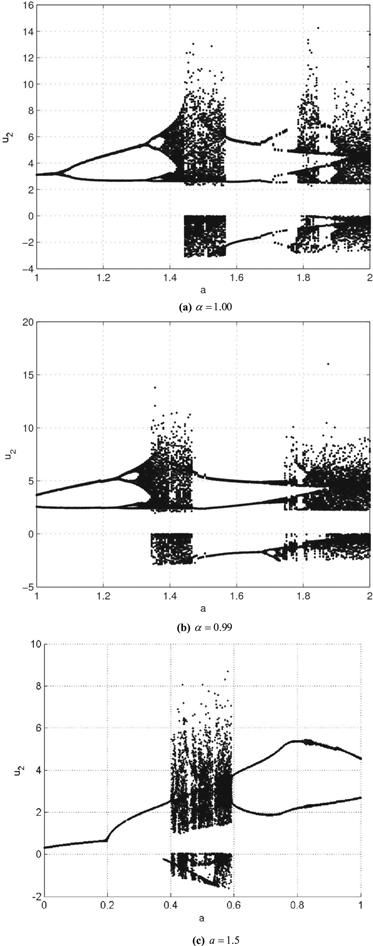
To verify the chaotic dynamics in system (8), topological structures, depicted by means of bifurcation maps, are calculated along the parameters $a,$ and $\alpha .$ In figures 1(a) and (b), these bifurcation maps, along with $a$ versus ${u}_{2}\left(t\right)$, are shown to be $\alpha =1.00$ and 0.99 respectively. It is evident in figures 1(a) and 1(b), that a periodic doubling trace appears when $a$ varies from 1 to 2, showing two distinct routes from $1\leqslant a\leqslant 1.5$ and $a\lt 2.$ The first route gives a clear picture of periodic doubling, but in the second route, the system loses chaotic oscillation. The parameter $a$ can therefore be used to control the degree of chaos. Interestingly, figure 1(c), analyzed in relation to system (8), shows a new bifurcation parameter $\alpha $ via a different route, with tangential and periodic doubling where $0\leqslant \alpha \leqslant 0.85$ and $0.85\lt \alpha \lt 1$, respectively.

Figure 1.

New window|Download| PPT slide
Figure 1.Bifurcation maps of system (8) for different parameters.


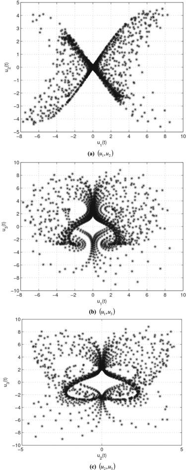
The trajectory of system (8) is calculated by means of the Poincaré section for co-dimensions in one phase space, as displayed in figures 2(a)-(c). Using equation (8), the dynamical waveforms are presented in figures 3-5 for well-defined initial conditions, and constant parameters, with each figure consisting of four sub-figures, (a)-(d). In figures 3(a)-(d), we have plotted the sequence of ${u}_{1}\left(t\right)$ at $\alpha =1.00,$ 0.99, 0.92, and 0.90, taking the time domain to be in the range of (0,300). The ${u}_{1}\left(t\right)$ for figure 3(a) is (−10,10), for figure 3(b) it is (−10, 10), figure 3(c) is (−10,7.5) and figure 3(d) is (−5,10). Similarly, with regard to different values of $\alpha ,$ sequences for ${u}_{2}\left(t\right)$ are plotted ,with the dynamics of figure 4(a) ranging from (−4,4) and in the same ranges for figures 4(b)-(d). Next, the ${u}_{3}\left(t\right)$ sequence for α= 1.00, 0.99, 0.92, 0.90 are shown to be (−10, 15), (−10, 10), (−10, 10) and (−5, 10), as presented in figures 5(a)-(d), respectively. Of all the figures discussed above, $\alpha =0.90$ exhibits the periodic waveform, and is in good agreement with the LE tabulated values given in table 2. In addition, we plotted a 2D phase where α= 1.00, 0.99, 0.92, 0.90 for the sequences $\left({u}_{1}\left(t\right),{u}_{2}\left(t\right)\right),$ $\left({u}_{1}\left(t\right),{u}_{3}\left(t\right)\right)$, and $\left({u}_{2}\left(t\right),{u}_{3}\left(t\right)\right)$ in figures 6(a)-(c), 7(a)-(c), and 8(a)-(c), respectively. Again, figures 6(d), 7(d) and 8(d) confirm non-chaotic behavior where α= 0.90, as predicted in table 2 on the basis of both LE and KYD. To provide further insight, the visualization of a 3D phase for (${u}_{1},{u}_{2},{u}_{3}$) has also been produced for different values of $\alpha $, as shown in figures 9(a)-(d). For the numerical validation of system (8), we implement the predictor corrector method (PCM) on system (1) with a step size pof 0.01. An absolute of log error is plotted in figures 10-12 for ${u}_{1}\left(t\right),$ ${u}_{2}\left(t\right)$ and ${u}_{3}\left(t\right)$, respectively, in which small values can be observed on the log scale.

Figure 2.

New window|Download| PPT slide
Figure 2.Poincaré section of system (8) at $\alpha =0.99.$

Figure 3.

New window|Download| PPT slide
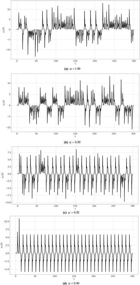
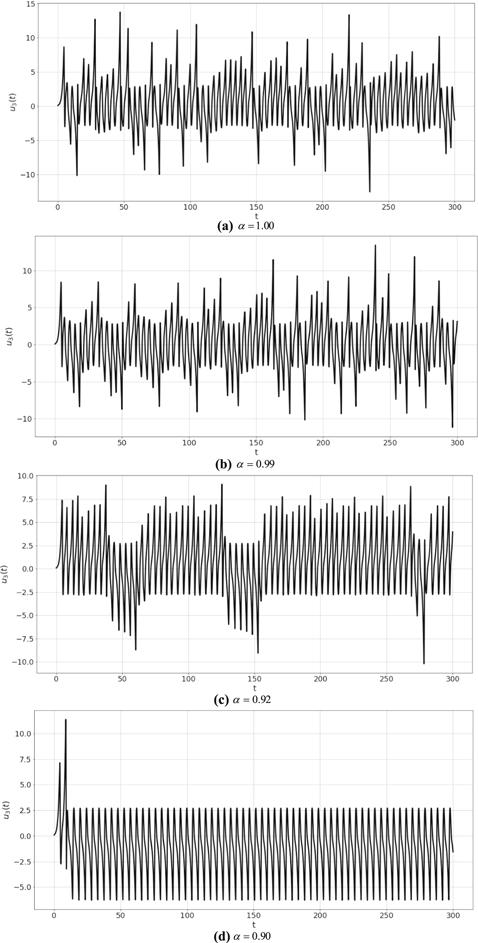
Figure 3.Plot ${u}_{1}\left(t\right)$ of system (8) for different values of $\alpha .$

Figure 4.

New window|Download| PPT slide
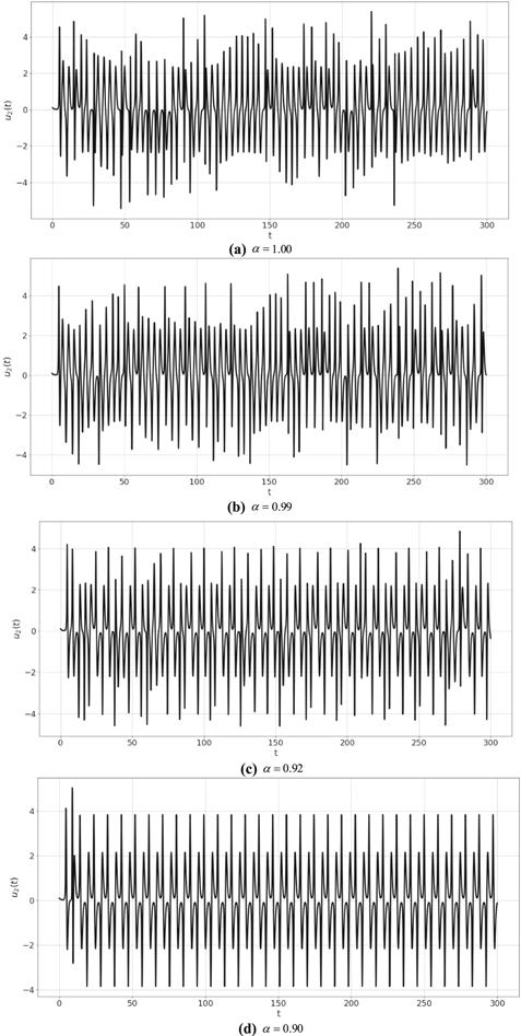
Figure 4.Plot ${u}_{2}\left(t\right)$ of system (8) at different values of $\alpha .$

Figure 5.

New window|Download| PPT slide
Figure 5.Plot ${u}_{3}\left(t\right)$ of system (8) for different values of $\alpha .$



Table 2.
Table 2.LE and KYD vakues for system (8).

$\alpha $	${L}_{1}$	${L}_{2}$	${L}_{3}$	${D}_{KY}$
1.00	0.266 697	−0.017 213	−4.695 504	2.053 13
0.99	0.273 420	−0.017 020	−4.804 732	2.053 36
0.92	0.003 342	−0.267 246	−3.945 491	1.933 11
0.90	0.000 167	−0.303 911	−3.942 772	1.922 96

New window|CSV

Figure 6.

New window|Download| PPT slide
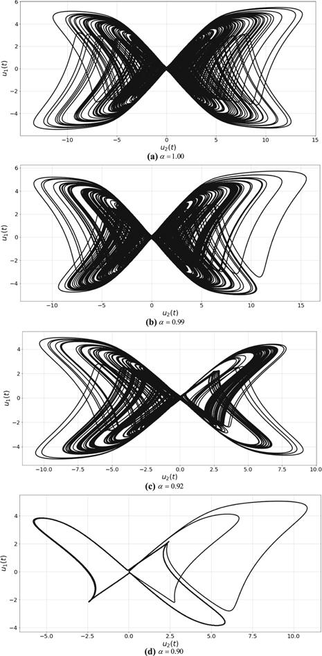
Figure 6.2D phase plot (${u}_{1},{u}_{2}$) of system (8) for different values of $\alpha .$

Figure 7.

New window|Download| PPT slide
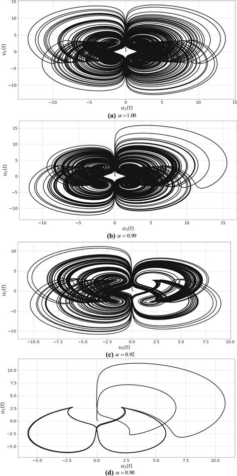
Figure 7.2D phase plot (${u}_{1},{u}_{3}$) of system (8) for different values of $\alpha .$

Figure 8.

New window|Download| PPT slide
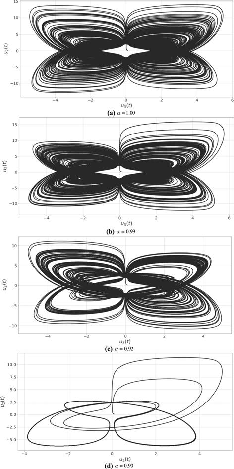
Figure 8.2D phase plot (${u}_{2},{u}_{3}$) of system (8) for different values of $\alpha .$

Figure 9.

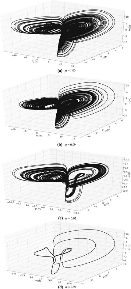New window|Download| PPT slide
Figure 9.3D flows of system (8) for different values of $\alpha .$

Figure 10.

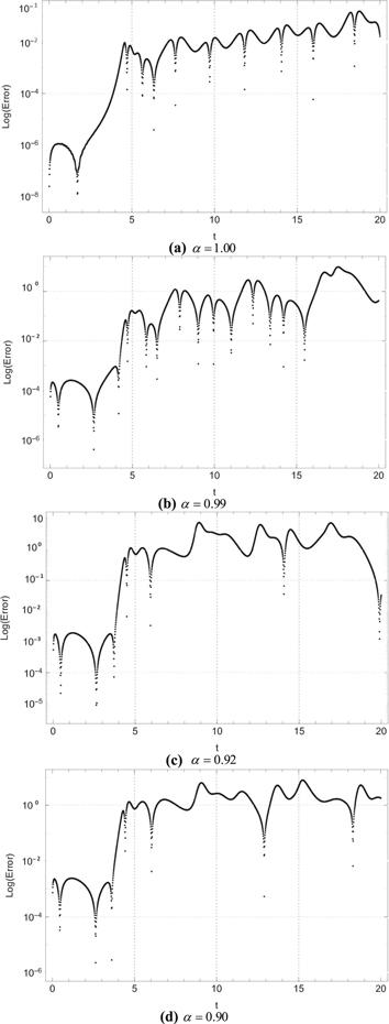New window|Download| PPT slide
Figure 10.Log errors for ${u}_{1}\left(t\right)$ between system (1) and system (8).

Figure 11.

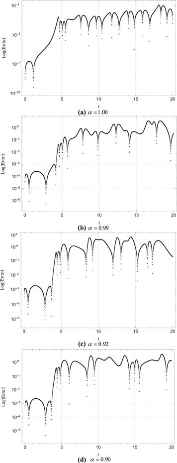New window|Download| PPT slide
Figure 11.Log errors for ${u}_{2}\left(t\right)$ between system (1) and system (8).

Figure 12.

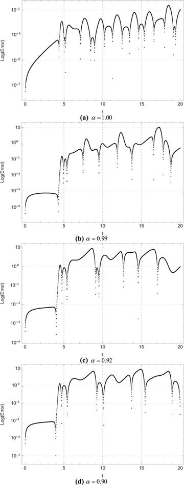New window|Download| PPT slide
Figure 12.Log errors for ${u}_{3}\left(t\right)$ between system (1) and system (8).

Figure 13.

New window|Download| PPT slide
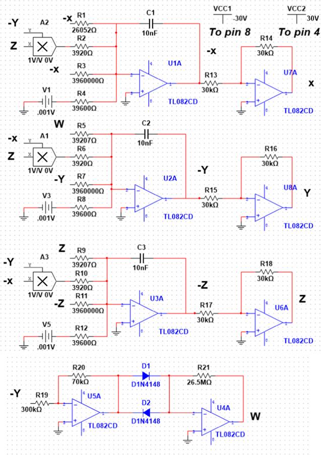
Figure 13.Schematic view of system (8), using MultiSIM 14.1.

4.2. Analog simulation

A circuit simulation for system (8) is presented in this section, with the help of the circuit equations shown below:(12)$\begin{eqnarray}\begin{array}{c}\begin{array}{l}{\dot{u}}_{1}\left(t\right)=-\displaystyle \frac{1.52}{{R}_{1}{C}_{1}}{u}_{1}\left(t\right)+\displaystyle \frac{1.01}{{R}_{2}{C}_{1}}{u}_{2}\left(t\right){u}_{3}\left(t\right)\\ \,\,\,-\,\displaystyle \frac{0.01}{{R}_{3}{C}_{1}}{u}_{1}\left(t\right)+\displaystyle \frac{0.001}{{R}_{4}{C}_{1}}{V}_{1},\\ {\dot{u}}_{2}\left(t\right)=-\displaystyle \frac{1.01}{{R}_{5}{C}_{2}}\,\sinh ({u}_{2}\left(t\right))+\displaystyle \frac{1.01}{{R}_{6}{C}_{2}}{u}_{1}\left(t\right){u}_{3}\left(t\right)\\ \,\,\,-\,\displaystyle \frac{0.01}{{R}_{7}{C}_{2}}{u}_{2}\left(t\right)+\displaystyle \frac{0.001}{{R}_{8}{C}_{2}}{V}_{2},\\ {\dot{u}}_{3}\left(t\right)=\displaystyle \frac{1.01}{{R}_{9}{C}_{3}}{u}_{3}\left(t\right)-\displaystyle \frac{1.01}{{R}_{10}{C}_{3}}{u}_{1}(t){u}_{2}\left(t\right)\\ \,\,\,-\,\displaystyle \frac{0.01}{{R}_{11}{C}_{3}}{u}_{3}\left(t\right)+\displaystyle \frac{0.001}{{R}_{12}{C}_{3}}{V}_{3},\end{array}\end{array}\end{eqnarray}$where ${C}_{i},$ ${R}_{j}$, and ${V}_{k}$ are the passive components, i.e. capacitor, resistor, and voltage DC source, respectively. The electronic circuit consists of twenty-one resistors, three capacitors, three multipliers (AD633JN), and six operational amplifiers (TL082CD) biased by a voltage of −30 V and 30 V. Three DC voltage sources are employed, and two semiconductor diodes (D1N4148) are used to create sine-hyperbolic conditions (see figure 13). The circuit design and simulation are successfully tracked via MultiSIM 14.1, and all results are acquired using three oscilloscopes: U1A (X signal), U2A (Y signal) and U3A (Z signal), respectively. The calculations for circuit components with different values of $\alpha $, are shown in table 3, and the conditions where α=1.00 and α=0.99 are depicted in figures 14 and 15, respectively, in order to ensure that our fractional calculations are in good agreement with those for integers. Figures 14 and 15 represent the 2D phase (${\rm{X}}$-${\rm{Y}}$ signal), (${\rm{Y}}$-${\rm{Z}}$ signal), and (${\rm{X}}$-${\rm{Z}}$ signal) for figures 14-15(a)-(c), respectively, and depict characteristic four-wing attractor behavior.


Table 3.
Table 3.The values of resistors and voltages for capacitors ${C}_{1}={C}_{2}={C}_{3}=10\,{\rm{nF}}$ for different values of $\alpha .$

$\alpha $	Voltage (${\rm{V}}$)		Resistor ($k{\rm{\Omega }}$)		$\alpha $	Voltage (${\rm{V}}$)		Resistor ($k{\rm{\Omega }}$)
1.00	${V}_{1}$	—	${R}_{1}$	20	0.92	${V}_{1}$	0.009	${R}_{1}$	24.29
			${R}_{2}$	3				${R}_{2}$	3.63
			${R}_{3}$	30				${R}_{3}$	440
	${V}_{2}$	—	${R}_{4}$	3		${V}_{2}$	0.009	${R}_{4}$	39.60
			${R}_{5}$	30				${R}_{5}$	36.33
			${R}_{6}$	3				${R}_{6}$	3.63
	${V}_{3}$	—	${R}_{7}$	—		${V}_{3}$	0.009	${R}_{7}$	440
			${R}_{8}$	—				${R}_{8}$	39.60
			${R}_{9}$	—				${R}_{9}$	36.33
			${R}_{10}$	—				${R}_{10}$	3.63
			${R}_{11}$	—				${R}_{11}$	440
			${R}_{12}$	—				${R}_{12}$	39.60
0.99	${V}_{1}$	0.001	${R}_{1}$	26.05	0.90	${V}_{1}$	0.011	${R}_{1}$	23.76
			${R}_{2}$	3.92				${R}_{2}$	35.64
			${R}_{3}$	3960				${R}_{3}$	356.75
	${V}_{2}$	0.001	${R}_{4}$	39.60		${V}_{2}$	0.011	${R}_{4}$	39.60
			${R}_{5}$	39.20				${R}_{5}$	35.64
			${R}_{6}$	3.920				${R}_{6}$	3.564
	${V}_{3}$	0.001	${R}_{7}$	3960		${V}_{3}$	0.011	${R}_{7}$	356.75
			${R}_{8}$	39.60				${R}_{8}$	39.60
			${R}_{9}$	39.20				${R}_{9}$	35.64
			${R}_{10}$	3.92				${R}_{10}$	3.564
			${R}_{11}$	3960				${R}_{11}$	356.75
			${R}_{12}$	39.60				${R}_{12}$	39.60

New window|CSV

Figure 14.

New window|Download| PPT slide
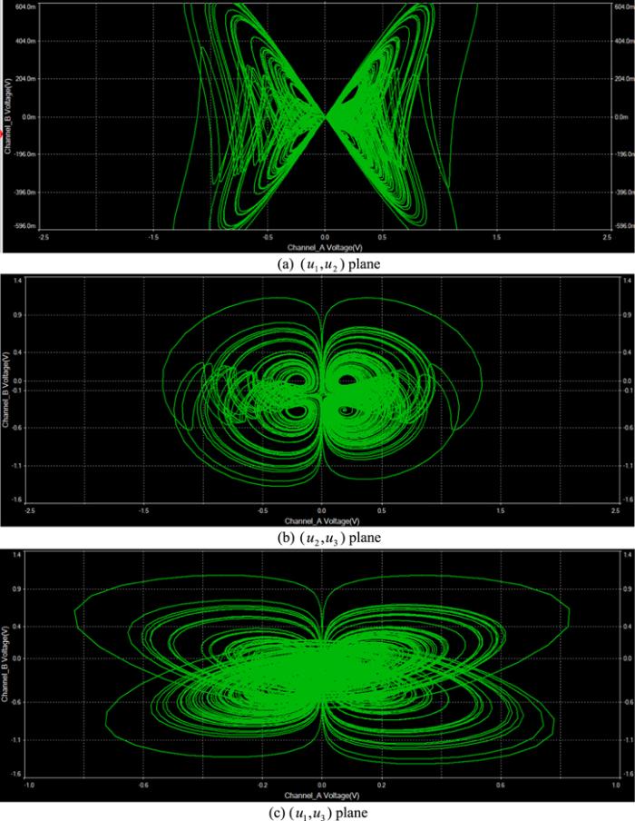
Figure 14.Analogous phase plots of system (8) where $\alpha =1.00.$

Figure 15.

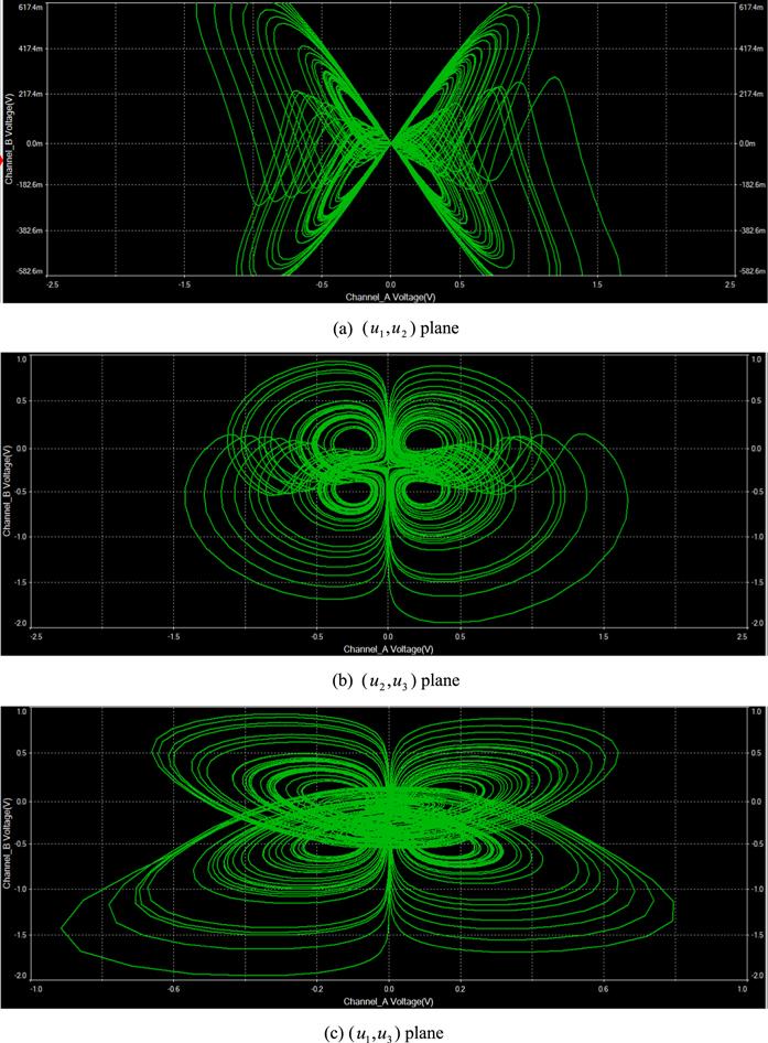New window|Download| PPT slide
Figure 15.Analogous phase plots of system (8) where $\alpha =0.99.$

4.3. Cryptographic simulation

This section considers the cryptography of voice, image, and animation data, using random number generation (RNG) produced via the solution given by our system (10). The system solution results were tested via NIST-800-22 [31], a rigorous statistical test used in chaotic systems to investigate the consistency of RNG [31] via the calculation of P-values. Here, P-values are given in tables 4-6 for equation (8), ${u}_{1}\left(t\right),$ ${u}_{2}\left(t\right)$, and ${u}_{3}\left(t\right)$, where α= 1.00, 0.99, and 0.92, respectively. The successful calculation and testing indicate the readiness of our system for encryption purposes; we therefore applied it to voice (figures 16-19), images (figures 20-23), and 12 animated (.gif) frames (presented in figure 24). Firstly, we encrypted voice data, using the RNG algorithm shown in figures 16(a)-(c); in order to ensure variations in the encryption, we plotted their magnitude spectrum (MS), power spectrum density (PSD), and spectrogram, as shown in figures 17-19, respectively. Secondly, we encrypted two images using RGB: one is Mandrill, depicted in figure 20, and the other is Peppers, as shown in figure 22, along with their histograms shown in figures 21 and 23, respectively. The results are in good agreement, as illustrated by the image captions original, encrypted, and decrypted. Lastly, the RNG algorithm was run for animation (.gif) in Python. The Python program is designed to produce original, encrypted, and decrypted files as output, on completion of the program [32]. The animated (gif.) encryption in relation to the individual frames of the animations (.gif), along with their histograms, are shown in figure 24. For reference, the relevant Python code may be found on the second author's web page in [32].


Table 4.
Table 4.${\rm P}$-value test results (NIST-800-22) for chaotic series ${u}_{1}\left(t\right),$ at different values of $\alpha .$

S. No	Test Name	$\alpha $=1	$\alpha $=0.99	$\alpha $=0.92	Results
1	Mono bitFrequency Test	0.665 006	0.484 806	0.317 884	Successful
2	Block Frequency Test	0.678 612	0.985 867	0.518 35	Successful
3	Runs Test	0.707 856	0.193 446	0.360 131	Successful
4	Longest Runs Ones 10 000	0.235 903	0.556 629	0.063 0856	Successful
5	Binary Matrix Rank Test	0.443 084	0.298 222	0.045 5016	Successful
6	Spectral Test	0.474 456	1.	0.458 246	Successful
7	Non-Overlapping Template Matching	0.529 55	0.840 569	0.488 286	Successful
8	Overlaping Template Matching	0.544 82	0.981 736	0.375 187	Successful
9	Maurers universal Statistic Test	0.463 56	0.183 854	0.385 959	Successful
10	Linear Complexity Test	0.701 088	0.515 697	0.503 53	Successful
11	Serial Test	{0.259 896,0.713 345}	{0.326 326,0.718 48}	{0.760 873,0.839 907}	Successful
12	Approximate Entropy Test	0.344 719	0.223 394	0.141 817	Successful
13	Cumulative Sums Test	0.638 251	0.825 325	0.593 75	Successful
14	Random Excursions Test	0.296 283	0.194 65	0.123 997	Successful
15	Random Excursions Variant Test	1	0.245 779	0.863 832	Successful
16	Cumulative Sums Test Reverse	0.976 076	0.822 779	0.593 75	Successful

New window|CSV


Table 5.
Table 5. ${\rm P}$-value test results (NIST-800-22) for chaotic series ${u}_{2}\left(t\right),$ at different values of $\alpha .$

S. No	Test Name	$\alpha $=1	$\alpha $=0.99	$\alpha $=0.92	Results
1	Mono bitFrequency Test	0.716 059	0.953 96	0.367 766	Successful
2	Block Frequency Test	0.638 647	0.474 88	0.617 961	Successful
3	Runs Test	0.004 748 35	0.567 602	0.784 317	Successful
4	Longest Runs Ones 10 000	0.692 827	0.933 756	0.377 388	Successful
5	Binary Matrix Rank Test	0.332 02	0.180 156	0.903 766	Successful
6	Spectral Test	0.289 315	0.524 923	0.542 336	Successful
7	Non-Overlapping Template Matching	0.873 754	0.329 533	0.137 408	Successful
8	Overlaping Template Matching	0.366 99	0.422 48	0.279 795	Successful
9	Maurers universal Statistic Test	0.336 621	0.535 156	0.844 607	Successful
10	Linear Complexity Test	0.229 947	0.969 042	0.224 795	Successful
11	Serial Test	{0.235 703,0.593 431}	{0.574 309,0.443 98}	{0.864 631,0.918 161}	Successful
12	Approximate Entropy Test	0.023 8884	0.586 246	0.249 462	Successful
13	Cumulative Sums Test	0.983 936	0.840 404	0.627 666	Successful
14	Random Excursions Test	0.769 331	0.804 348	0.316 433	Successful
15	Random Excursions Variant Test	0.947 793	0.388 667	0.331 918	Successful
16	Cumulative Sums Test Reverse	0.727 184	0.788 972	0.263 668	Successful

New window|CSV


Table 6.
Table 6.${\rm P}$-value test results (NIST-800-22) for chaotic series ${u}_{3}\left(t\right),$ at different values of $\alpha .$

S. No	Test Name	$\alpha $=1	$\alpha $=0.99	$\alpha $=0.92	Results
1	Mono bitFrequency Test	0.981 575	0.623 605	0.724 701	Successful
2	Block Frequency Test	0.702 138	0.786 538	0.330 245	Successful
3	Runs Test	0.145 69	0.463 838	0.724 432	Successful
4	Longest Runs Ones 10 000	0.746 165	0.415 693	0.423 45	Successful
5	Binary Matrix Rank Test	0.685 773	0.574 195	0.570 329	Successful
6	Spectral Test	0.194 273	0.633 482	0.474 456	Successful
7	Non-Overlapping Template Matching	0.834 296	0.498 41	0.512 831	Successful
8	Overlaping Template Matching	0.219 927	0.664 717	0.230 988	Successful
9	Maurers universal Statistic Test	0.235 758	0.139 78	0.688 589	Successful
10	Linear Complexity Test	0.709 004	0.523 366	0.803 015	Successful
11	Serial Test	{0.412 075,0.209 017}	{0.197 128,0.442 195}	{0.437 12,0.534 607}	Successful
12	Approximate Entropy Test	0.734 978	0.135 837	0.845 66	Successful
13	Cumulative Sums Test	0.845 347	0.770 349	0.791 612	Successful
14	Random Excursions Test	0.654 05	0.281 157	0.428 759	Successful
15	Random Excursions Variant Test	0.262 747	0.326 878	0.391 404	Successful
16	Cumulative Sums Test Reverse	0.825 325	0.360 73	0.635 598	Successful

New window|CSV

Figure 16.

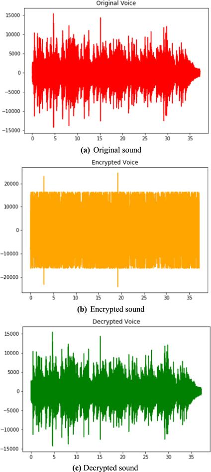New window|Download| PPT slide
Figure 16.Sound data.

Figure 17.

New window|Download| PPT slide
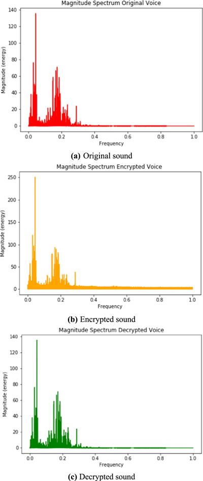
Figure 17.Magnitude spectrum of sound.

Figure 18.

New window|Download| PPT slide
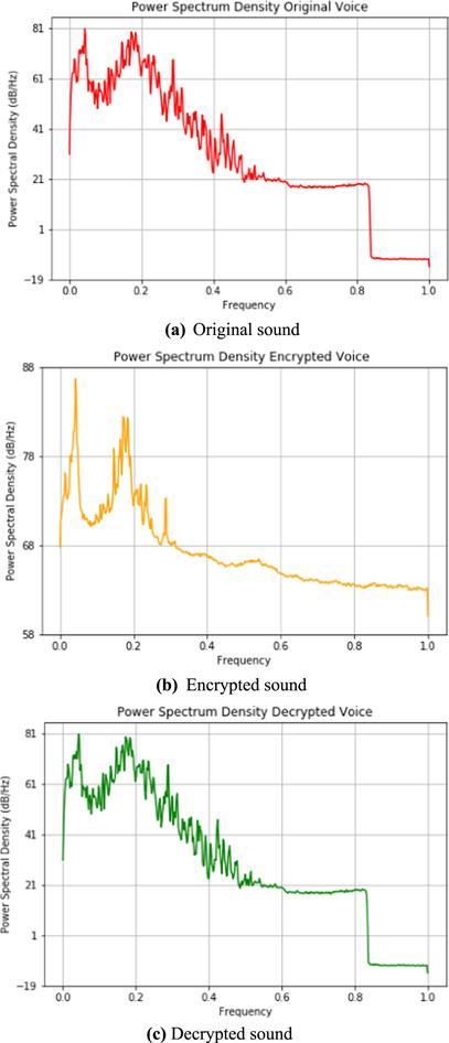
Figure 18.Power spectrum density of sound data.

Figure 19.

New window|Download| PPT slide
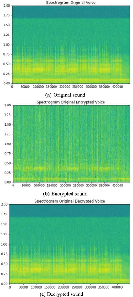
Figure 19.Spectrogram of sound data.

Figure 20.

New window|Download| PPT slide
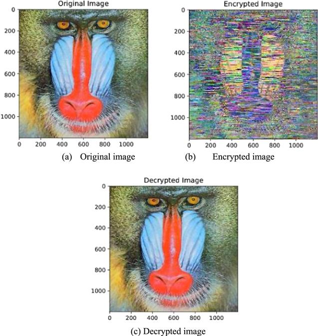
Figure 20.Cryptographic test on image 1 (Mandrill).

Figure 21.

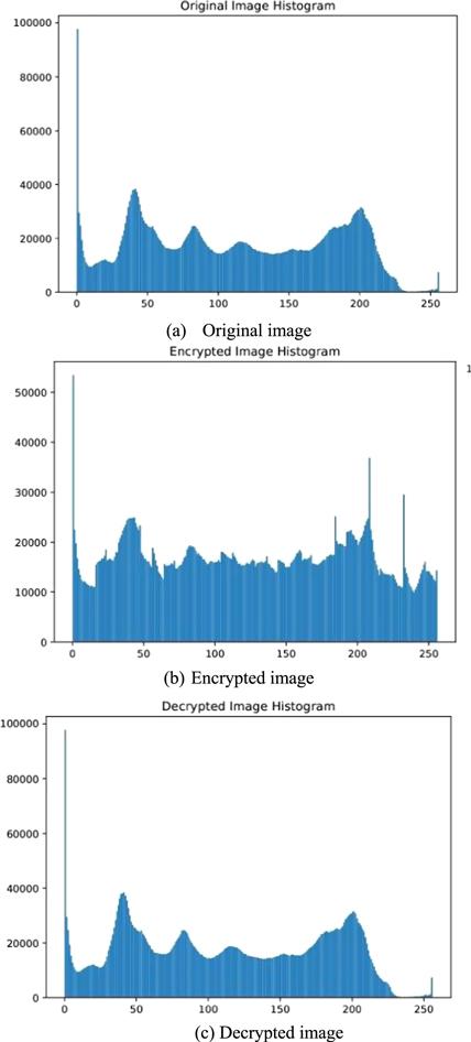
New window|Download| PPT slide
Figure 21.Histogram of cryptographic test on image 1.

Figure 22.

New window|Download| PPT slide
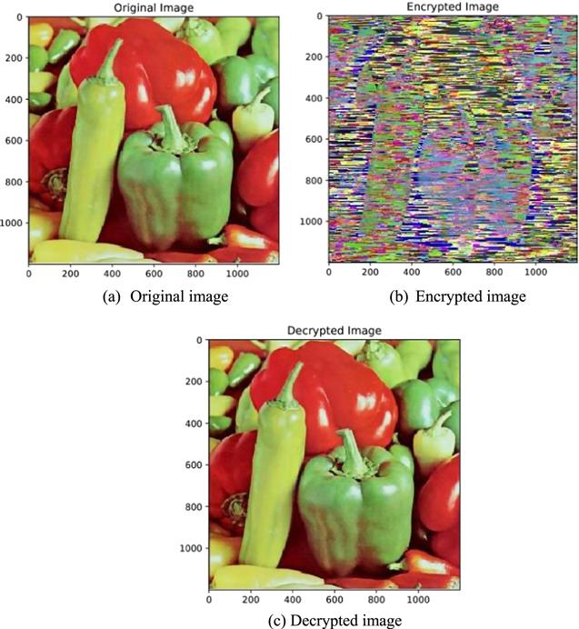
Figure 22.Cryptographic test on image 2 (Peppers).

Figure 23.

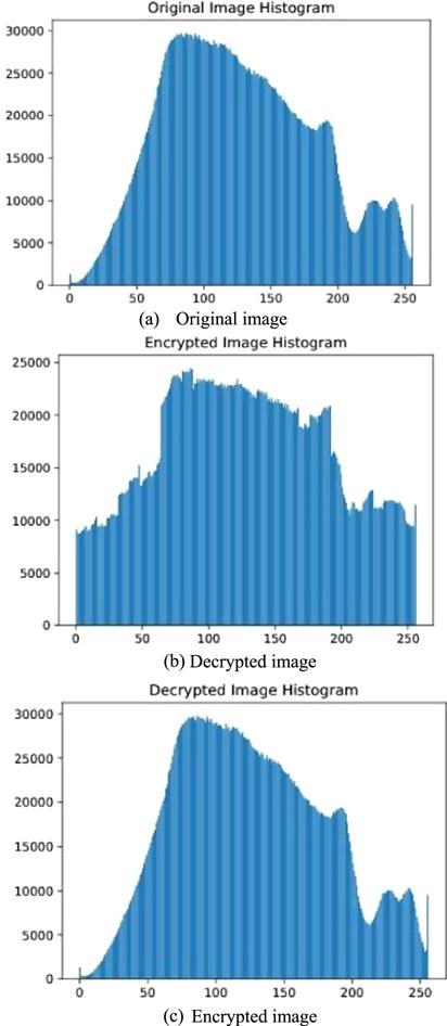
New window|Download| PPT slide
Figure 23.Histogram of cryptographic test on image 2.

Figure 24.

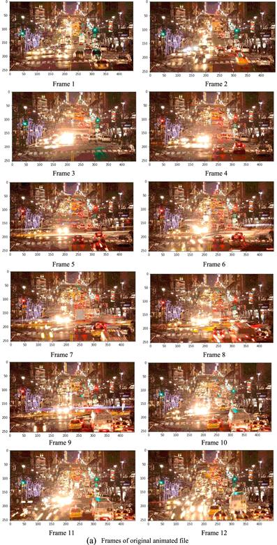New window|Download| PPT slide
Figure 24.Frames from an animated (.gif) file original, encrypted, and decrypted, together with the corresponding histograms.

4.4. Security analysis

In this section, the cryptosystem's sensitivity, as well as its capacity to withstand attack, are analyzed in relation to the test images, on the basis of the parameters shown below.

4.4.1. Histogram analysis

The statistical characteristics of the images are presented in the form of histograms. The original and encrypted images are analyzed in relation to the behavior of the graphs. The graph of encrypted image shows uniformity, which suggests us that the encryption is capable of resisting a statistical attack. Histograms for the Mandrill and Pepper images are provided in figures 21 and 23, respectively.

4.4.2. Key sensitivity analysis

Small changes in the secret key, which alter the encryption image, are indicative of key sensitivity. The two parameters, NPCR and UAIC, are used to measure key sensitivity, and are discussed below:1.NPCR:The number of pixel change rate (NPCR) can be expressed as follows:$\begin{eqnarray*}\begin{array}{l}{\rm{N}}{\rm{P}}{\rm{C}}{\rm{R}}=\displaystyle \sum _{i=1}^{M}\displaystyle \sum _{j=1}^{N}\left[\displaystyle \frac{D\left(i,j\right)}{M\times N}\right]\times 100 \% ,\,{\rm{with}}\\ D\left(i,j\right)=\left\{\begin{array}{cc}0 & {C}_{1}\left(i,j\right)={C}_{2}\left(i,j\right)\\ 1 & otherwise\end{array}\right..\end{array}\end{eqnarray*}$Here, ${C}_{1}\left(i,j\right)$ and ${C}_{2}\left(i,j\right)$ denote the pixel values of the two encrypted images, where the originals possess only one pixel difference, respectively, at the ith pixel row,and the jth pixel column.
2.UACI: The unified average changing intensity (UACI) can be written as follows:
$\begin{eqnarray*}{\rm{U}}{\rm{A}}{\rm{C}}{\rm{I}}=\displaystyle \sum _{i=1}^{M}\displaystyle \sum _{j=1}^{N}\left[\displaystyle \frac{\left|{C}_{1}\left(i,j\right)-{C}_{2}\left(i,j\right)\right|}{255\times M\times N}\right]\times 100 \% .\end{eqnarray*}$

4.4.2.1. Information entropy analysis

1. Entropy indicates the randomness of a system, and can be calculated as follows:
$\begin{eqnarray*}e\left(m\right)=\displaystyle \sum _{i=0}^{{2}^{N}-1}p\left({m}_{i}\right)\times {\mathrm{log}}_{2}\left(\displaystyle \frac{1}{p\left({m}_{i}\right)}\right)\end{eqnarray*}$here, $p\left({m}_{i}\right)$ denotes the probability of messages ${m}_{i}.$

The mean number of pixels in the Mandrill and Peppers images are assumed to be 98.958 079 and 99.104 309, respectively, indicating that these images differ by only one pixel. Meanwhile, the UACI values indicate the absence of significant change between the test images used in the study. Analyses conducted by means of these parameters are performed on the two test images, and the results are tabulated in table 7. The correlations of original and encrypted images of the Mandrill image are 0.924 877 and 0.861 089, respectively, and those for the Peppers image are 0.956 570 and 0.934 504, respectively, indicating that the images are neither identical nor opposite. Furthermore, table 7 clearly shows that the entropy of the original image is less than the entropy of the encrypted image; hence, rare uncertainty transmits.


Table 7.
Table 7.Numerical values of Parameters for security analysis.

			Entropy
Test images	NPCR (%)	UAIC (%)	Plain Image	Encrypted Image
Mandrill	98.958 079	21.426 310	5.333 076	5.777 796
Peppers	99.104 309	24.509 208	4.342 038	5.742 104

New window|CSV

5. Conclusion

This paper presents a four-wing chaotic attractor system, having sine-hyperbolic nonlinearity, and incorporating FDs. This fusion of FDEs has vast implications in terms of the secure encryption of different types of data, such as voice, image, and animated images, which are ubiquitous in digital communication. The equations are tested numerically and via electronic simulation, using Mathematica and MultiSIM, respectively. Numerical results are simulated for different values of $\alpha $ in order to confirm the validity of this multi-wing chaotic system. The cryptographical element is coded in Python, and is tested on audio, image, and animated gif files. The study offers the following conclusions:• The multi-wing system possesses multi-stability equilibrium points at distinct values of $\alpha .$
• The physical parameters of the model can be simulated by means of circuit design.
• Many keys can be generated to form sheltered systems for data communication.
• The proposed mechanism has the capacity to track files in different formats.
• This system is also suitable for other chaos-based applications.

Reference View Option By original order
By published year
By cited within times
By Impact factor

[1]Kilbas A A A Srivastava H M Trujillo J J 2006 Theory and Applications of Fractional Differential Equations vol 204 Amsterdam Elsevier
[Cited within: 3]

[2]Podlubny I 1998 Fractional differential equations
Mathematics in Science and Engineering vol 198 New York Elsevier
[Cited within: 2]

[3]Tarasov V E 2013 No violation of the Leibniz rule. No fractional derivative
Commun. Nonlinear Sci. Numer. Simul. 18 2945 2948
DOI:10.1016/j.cnsns.2013.04.001 [Cited within: 1]

[4]Tarasov V E 2018 No nonlocality. No fractional derivative
Commun. Nonlinear Sci. Numer. Simul. 62 157 163
DOI:10.1016/j.cnsns.2018.02.019 [Cited within: 1]

[5]Lorenz E N 1963 Deterministic nonperiodic flow
J. Atmos. Sci. 20 130 141
DOI:10.1175/1520-0469(1963)020<0130:DNF>2.0.CO;2 [Cited within: 1]

[6]Pham V-T Volos C K Vaidyanathan S 2015 Multi-scroll chaotic oscillator based on a first-order delay differential equation
Chaos Modeling and Control Systems Design Berlin Springer 59 72
DOI:10.1007/978-3-319-13132-0_4 [Cited within: 1]

[7]Khan N A et al. 2020 Emulate the chaotic flows of fractional jerk system to scramble the sound and image memo with circuit execution
Phys. Scr. 95 065217
DOI:10.1088/1402-4896/ab8581 [Cited within: 1]

[8]Sarwar S Iqbal S 2018 Stability analysis, dynamical behavior and analytical solutions of nonlinear fractional differential system arising in chemical reaction
Chin. J. Phys. 56 374 384
DOI:10.1016/j.cjph.2017.11.009 [Cited within: 1]

[9]Zhang J Liao X 2017 Synchronization and chaos in coupled memristor-based FitzHugh-Nagumo circuits with memristor synapse
AEU-Int. J. Elec. Commun. 75 82 90
DOI:10.1016/j.aeue.2017.03.003 [Cited within: 1]

[10]Wu G-C Baleanu D Lin Z-X 2016 Image encryption technique based on fractional chaotic time series
J. Vib. Control 22 2092 2099
DOI:10.1177/1077546315574649 [Cited within: 1]

[11]Yildirim A et al. 2011 Analysis of nonlinear oscillations of a punctual charge in the electric field of a charged ring via a Hamiltonian approach and the energy balance method
Comput. Math. Appl. 62 486 490
DOI:10.1016/j.camwa.2011.05.029 [Cited within: 1]

[12]Yıldırım A Koçak H 2012 A more approximate green's function for the electric field vector with anisotropic properties
J. Electromagn. Waves Appl. 26 24 33
DOI:10.1163/156939312798954964 [Cited within: 1]

[13]Chen L et al. 2016 Design and implementation of grid multi-scroll fractional-order chaotic attractors
Chaos 26 084303
DOI:10.1063/1.4958717 [Cited within: 1]

[14]Chen L et al. 2016 Generation and circuit implementation of fractional-order multi-scroll attractors
Chaos Solitons Fractals 85 22 31
DOI:10.1016/j.chaos.2016.01.016 [Cited within: 1]

[15]Chen L et al. 2017 Generation of a family of fractional order hyper-chaotic multi-scroll attractors
Chaos Solitons Fractals 105 244 255
DOI:10.1016/j.chaos.2017.10.032 [Cited within: 1]

[16]Khan N A et al. 2019 Tracking the chaotic behaviour of fractional-order Chua's system by Mexican hat wavelet-based artificial neural network
J. Low Freq. Noise Vibration Active Control 38 1279 1296
DOI:10.1177/1461348418813015 [Cited within: 1]

[17]Elwakil A S Ozoguz S Kennedy M P 2002 Creation of a complex butterfly attractor using a novel Lorenz-type system
IEEE Trans. Circuits Syst. I 49 527 530
DOI:10.1109/81.995671 [Cited within: 1]

[18]Elwakil A S Özoǧuz S Kennedy M P 2003 A four-wing butterfly attractor from a fully autonomous system
Int. J. Bifurcation Chaos 13 3093 3098
DOI:10.1142/S0218127403008405 [Cited within: 1]

[19]Zidan M A Radwan A G Salama K N 2012 Controllable V-shape multiscroll butterfly attractor: system and circuit implementation
Int. J. Bifurcation Chaos 22 1250143
DOI:10.1142/S021812741250143X [Cited within: 1]

[20]Zhang C Yu S 2013 On constructing complex grid multi‐wing hyperchaotic system: theoretical design and circuit implementation
Int. J. Circuit Theory Appl. 41 221 237
DOI:10.1002/cta.736 [Cited within: 1]

[21]Yu S et al. 2010 Design and implementation of multi-wing butterfly chaotic attractors via Lorenz-type systems
Int. J. Bifurcation Chaos 20 29 41
DOI:10.1142/S0218127410025387 [Cited within: 1]

[22]Qi G et al. 2008 A four-wing chaotic attractor generated from a new 3D quadratic autonomous system
Chaos Solitons Fractals 38 705 721
DOI:10.1016/j.chaos.2007.01.029 [Cited within: 1]

[23]Huang Y 2014 A family of multi-wing chaotic attractors and its circuit implementation
Acta Phys. Sin. 63 080505
DOI:10.7498/aps.63.080505 [Cited within: 1]

[24]Lü J Chen G 2006 Generating multiscroll chaotic attractors: theories, methods and applications
Int. J. Bifurcation Chaos 16 775 858
DOI:10.1142/S0218127406015179 [Cited within: 1]

[25]Wang Z et al. 2017 Four-wing attractors in a novel chaotic system with hyperbolic sine nonlinearity
Optik 131 1071 1078
DOI:10.1016/j.ijleo.2016.12.016 [Cited within: 1]

[26]Ren J Sun Z Z Dai W 2016 New approximations for solving the Caputo-type fractional partial differential equations
Appl. Math. Modell. 40 2625 2636
DOI:10.1016/j.apm.2015.10.011 [Cited within: 1]

[27]Moysis L et al. 2019 Analysis, synchronization and microcontroller implementation of a generalized hyperjerk system, with application to secure communications using a descriptor observer
2019 Panhellenic Conf. on Electronics & Telecommunications (PACET) Greece IEEE
DOI:10.1109/PACET48583.2019.8956261 [Cited within: 1]

[28]Keshtkar F Kheiri H Erjaee G 2014 Fixed points classification of nonlinear fractional differential equations as a dynamical system
J. Fractional Calculus Appl. 5 59 70
[Cited within: 1]

[29]Wolf A et al. 1985 Determining Lyapunov exponents from a time series
Physica D 16 285 317
DOI:10.1016/0167-2789(85)90011-9 [Cited within: 1]

[30]Kaplan J L Yorke J A 1979 Chaotic behavior of multidimensional difference equations
Functional Differential Equations and Approximation of Fixed Points Lecture Notes in MathematicsPeitgen H O Walther H O vol 730 Berlin Springer
[Cited within: 1]

[31]Rukhin A et al. 2011 A Statistical Test Suite for Random and Pseudorandom Number Generators for Cryptographic Applications Gaithersburg National Institute of Standards and Technology MD 20899-8930
[Cited within: 2]

[32]Qureshi M A 2020 Encryption-Python-Codes: Release of Voice and Image Encryption in Python Zenodo
DOI:10.5281/zenodo.3693098 [Cited within: 2]