 ,1,?, Liang-Wei Dong1, Hai-Feng Li2
 Corresponding authors: ?Corresponding author, E-mail:qiwei@sust.edu.cn
Received:2019-02-8Online:2019-07-1
| Fund supported: |

Abstract
Keywords:
PDF (253KB)MetadataMetricsRelated articlesExportEndNote|Ris|BibtexFavorite
Cite this article
Wei Qi, Liang-Wei Dong, Hai-Feng Li. Effects of Quantum Fluctuations on $\mathcal{PT}$-Symmetric Solitons of a Trapped Bose Gas *. [J], 2019, 71(7): 773-778 doi:10.1088/0253-6102/71/7/773
Introduction
Isolated quantum systems are governed by unitarydynamics and described by Hermitian Hamiltonians, yetthe interaction with the environment often plays animportant role in studies of ultracold atoms, leading to gainor loss of particles. In the mean-field approximation ofthe Gross-Pitaevskii (GP) equation, the necessary particle gain andloss can be described by imaginary potentials, renderingthe Hamiltonian non-Hermitian.[1-2] Theparticle in- and out-coupling were compared to many-particlecalculations justifying their use in mean-field theory.[3-4] In 1998 Bender and Boettcher[5] discovered that non-Hermitian Hamiltonians can support stationary solutions if they are $\mathcal{PT}$ symmetric.Based on this, $\mathcal{PT}$ symmetry is applied to the nonlinear GP equationto describe a dilute Bose-Einstein condensate (BEC).[6] $\mathcal{PT}$-symmetry implies the complex potential $V(x)$ contained in GP equation satisfies the condition: $V(x)=V^{*}(-x)$. In such a system the imaginary part of the potential represents thein- and out-coupling of particles into or from an external environment. Many interesting nonlinear phenomena have been recovered in this $\mathcal{PT}$-symmetric BEC system. For example: Nonlinear $\mathcal{PT}$-symmetric quantum systems have been discussed for BEC described in a two-mode approximation;[7-8] the studies of the nonlinear quantum dynamics in a $\mathcal{PT}$ double well,[9] vortices in BEC with a $\mathcal{PT}$-symmetric potential.[10] Meanwhile, $\mathcal{PT}$ symmetry has found applications in several areas, it has been recently recognized that optics can provide a fertile ground where$\mathcal{PT}$-symmetric concepts can be fruitfully exploited.[11-13] And some interesting works about $\mathcal{PT}$-symmetry-induced high-sensitivity refractive index sensors in optical solid state materials, such as coupled gain-loss microcavities have been reported. For example, a side-coupled cavity array structure has recently been explored in a $\mathcal{PT}$-symmetric context for sensor applications.[14]We know that in cold atomic systems, interactions also play a key role in its nonlinear dynamics properties. Except in thelimit of weak interactions, where a mean-field approach isoften sufficient, theories for interacting systems dominated by $s$-wave scattering length. Recently, it was pointed out that quantum fluctuationscan stabilize a dipolar BEC[15-19] and Bose-Bose mixture.[20-21] Furthermore,a quantum droplet can be formed, which would otherwise collapse under attractive mean-field forces.Though tuning the atom numbers and interactions in a Bose-Bose mixture to cancel mean-field interactionscompletely, a novel approach to studying quantum fluctuations has been presented in Ref. [22]. Moreover, it is shown with the help of quantum fluctuations, a supersolid phase can occur in dipolar BEC.[23]
Bright solitons and quantum droplets are two distinct boundstates in BEC. Solitons require the gas to remain effectively one-dimensional.[24-25] In contrast,droplets are three-dimensional solutions that exist even infree space.[26-27] Recently, considering the quantum fluctuations, the static and dynamic properties of a trapless 1D BEC have been carefully studied.[28] However, combing the particles gain and loss mechanisms, how the the quantum fluctuations affect the existence andstability properties of the solitons is still absent. Our results show that the quantum fluctuations can dramatically influence the $\mathcal{PT}$-symmetric soliton's localization and stability properties.
The paper is organized as follows. In Sec. 2, we present thephysical models. In Sec. 3, variational approach suitable for non-Hermitian systems is presented. In Sec. 4, we discuss the effects of quantum fluctuations on the density profile, width and chemical potential of the solitons. Meanwhile, using Vakhitov-Kolokolov (VK) stability criterion analytical, the effects of quantum fluctuations on the solitons stability properties are presented. In Sec. 5, we make our main conclusions.
2 Theoretical model
We consider a BEC with two-body and quantum fluctuation effects trapped in a $\mathcal{PT}$symmetry potential, the condensate wave function following modified GP equation:[22,29-30]where $\hbar$ is the reduced Planck's constant, $m$ is the mass of a single boson, $g_{0}=4\pi\hbar^{2}a/m$, $q_{0}=32g_{0}a^{3/2}/(3\sqrt{\pi})$.The $s$-wave scattering length $a$ corresponds to the lowest-order zero-range potential of the two-body contact interactions.$g_{0}$ is the strength of two-body contact interactions. The $q_{0}$ is the Lee Huang-Yang term[31] that accounts for the correction due to quantumfluctuations. Assuming that the condensate is harmonically trapped in the $y$ and $z$ directions and with an axial trap potential $V(x)$ in the direction $x$,the external trapping potential can be written as $V(\vec{r})=({1}/{2})m\omega_{\perp}(y^{2}+z^{2})+V(x)$. The radial motion can be strongly confined by making thethe radial trapping frequency $\omega_{\perp}\gg \omega_{x}$. In this case the condensate is cigar-shaped, and owing to that, one can take $\Psi(\vec{r},t)=\phi_{0}\psi(x,t)$, where $\phi_{0}=\sqrt{{1}/{\pi a_{\perp}^{2}}}\exp(-{r_{\perp}^{2}}/{2a_{\perp}^{2}})$ is the ground state of the radial problem, with $a_{\perp}=\sqrt{\hbar/(m\omega_{\perp})}$, and $r_{\perp}=\sqrt{y^{2}+z^{2}}$ being the radial distance. Then multiplying both sides of the modified GPequation Eq. (1) by $\phi_{0}^{*}$ and integrating over the transverse variable $r_{\perp}$, we obtain a quasi-one-dimensional GP equation in the form:
we rescale the wave function, space and times as follows:[32]
$$\tau=({1}/{2})\omega_{\perp}t\,, \quad \tilde{x}=a_{\perp}^{-1}x\,, \quad \tilde{\psi}=\sqrt{a_{\perp}^{-3}}\psi\,, \tilde{g_{0}}=({2a_{\perp}^{3}}/{\hbar \omega_{\perp}})g_{0}\,, \quad \tilde{q_{0}}=({2a_{\perp}^{9/2}}/{\hbar \omega_{\perp}})q_{0}\,,\tilde{V}(x)=V(x)/\hbar\omega_{\perp}\,.$$
We will continue to use $t$ instead of $\tau$, and we drop the tildes for simplicity. The dynamics of the cigar-shaped condensate can be governed by a quasi-1D GP equation, which have the dimensional form:
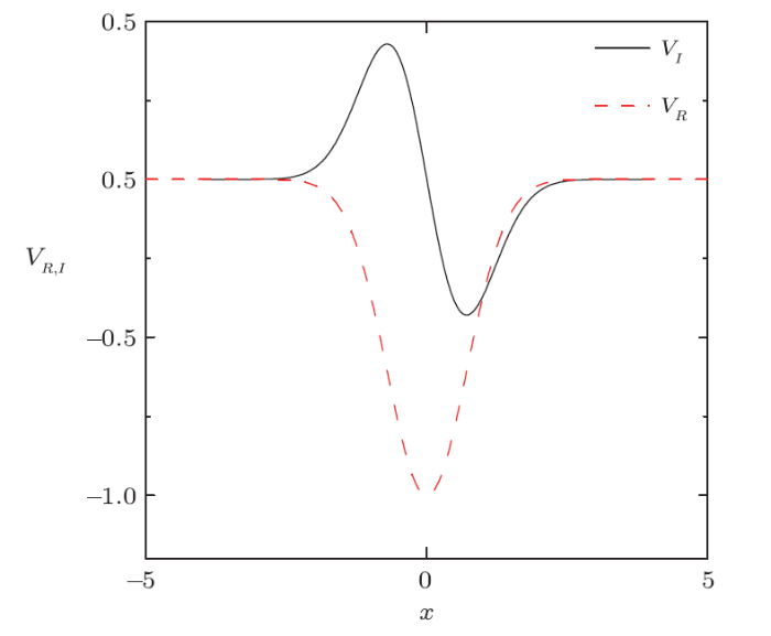
In Eq. (3) we take $ V(x)$ to be complex valued and $\mathcal{PT}$ symmetric, i.e., possessing a symmetric real part and an antisymmetric imaginary part. Thepotential has the form $V(x)=V_{R}(x)+{\rm i} V_{I}(x)$. We choose a Gaussian-shaped potential $V_{R}=-V_{r}\exp(-x^{2})$ as the real part of $\mathcal{PT}$ potential.Such trap can be implemented using optical dipole traps. The imaginary part is chosen as a Gaussian multiplied by $x$, expressed as $V_{I}=-V_{i}x\exp(-x^{2})$.Figure 1 depicts the real part and the imaginary part of $V(x)$, the imaginary part represents the gain-loss mechanisms.
Fig.1
 New window|Download| PPT slide
Fig.1(Color online) The transverse profiles of the real and imaginary part of the potential $V(x)$, the black solid line represents the imaginary part, the red dotted line is for the real part, with $V_{r}=V_{i}=1$.
3 Variational Approach
We are interested in devising a variational principle to obtain the equation of the wave function for the GP equation with a complex potential.However, the complexity of the potential makes the problem nonconservative. Here, we use the variational approach developed for dissipative systems. Inserting the ansatz $\psi=\phi(x)\exp(-\rm i \mu t)$ into Eq. (3), we getThe Lagrangian for the conservative part, corresponding to the left-hand side of Eq. (4), is
To apply the variational approach, we choose a trial solution with the nonzero phase associated with $\mathcal{PT}$-symmetric stationary states:
where $A$ corresponds to the condensate amplitude supposed to be real, $\omega_{b}$ is the width of the soliton, $\theta$ is the amplitude of thephase profile, and $f(x)$ is the phase distribution along $x$. The particle number of soliton is defined as $N=\int^{\infty}_{-\infty}|\phi|^{2}\rm d x=\sqrt{{\pi}/{2}}A^{2}\omega_{b}$. Inserting Eq. (6) into Eq. (5), we get the following Lagrangian:
From Eq. (7), we can obtain the following reduced Lagrangian $\langle L_{c}\rangle=\int^{\infty}_{-\infty}L_{c}\rm d x$ as
Eq. (8) can be further simplified and be rewritten in the term of particle number $N$, obtaining
The last two terms on the right-hand side of Eq. (9) depend on the square and $5/2$ power-law of the particle number $N$, stemming from the two-body interactionsand quantum fluctuations respectively. Using the standard variational approach for systems with dissipative terms can be modified as[29,33]
where $\varphi=N, \omega_{b}, \theta$. With $Q=\rm i V_{I}(x)\phi$ representing the gain-loss of particle from environment.
Choosing $\varphi=N$, from Eq. (10) we can obtain an explicit expression for the chemical potential $\mu$ as
The first term on the right-hand of Eq. (11) stems from the influence of the phase profile $\theta f(x)$ on the nonlinear eigenvalue $\mu$. The second term stems from the dispersive spreading. The third and forth terms originate from two-body interaction and quantum fluctuation effects, respectively. It is clearly shown that they have competition relationship between two-body interactions and quantum fluctuations on chemical potential. The last term in Eq. (11) accounts for the contribution of the linear trapping potential $V_{R}$.
Secondly, when we choose $\varphi=\omega_{b}$, from Eq. (10) we obtain
The left-hand side of Eq. (12) states the competition among dispersion of the particles (first term), two-body interactions (second term), and quantum fluctuations (third term) to determine the condensate width if the trapping potential is absent. From the expression of Eq. (12), it expresses that the quantum fluctuations dramatically influence the condensate width. The first term on the right-hand of Eq. (12) arises from the inhomogeneous phase of the soliton. While the second term of Eq. (12) in right-hand accounts for the influence of the linear trapping potential on the condensate width.
Finally, the equation for $\theta$ is obtained by choosing $\varphi=\theta$, from this we obtain
From Eq. (13), we can see that the phase of the soliton is immune from atomic interaction. For purely real potentials ($V_{I}=0$), stationary solutions feature a flat phase profile across $x$.
In the following, using the variational results, we focus on how the quantum fluctuations influence on the properties of soliton. For mainly investigating the effects of quantum fluctuations on bright solitons properties, we will be interested in the particular case of two-body interaction $g_{0}=-1$.
4 Discussion
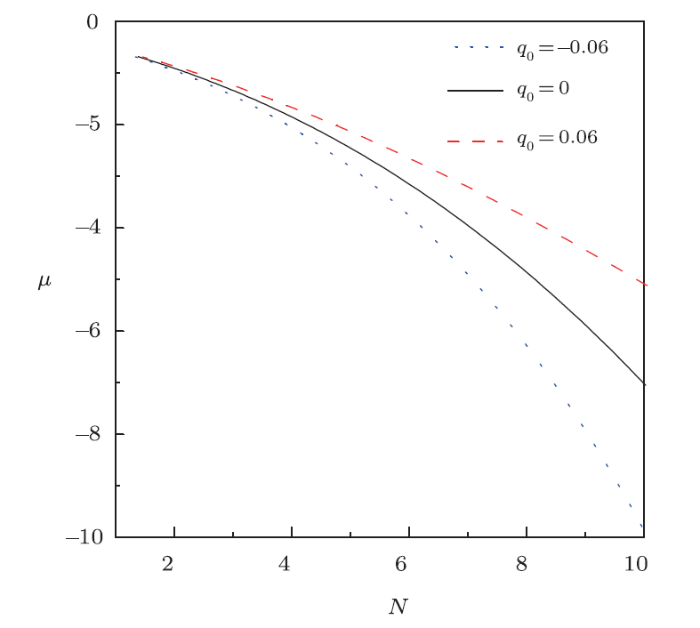
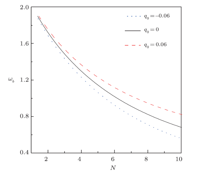
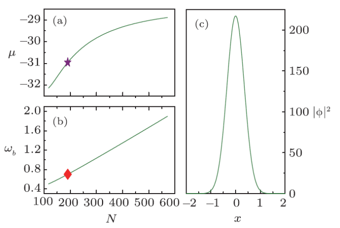
In our variational analysis, we choose $f(x)=\tanh(x)$ into Eq. (6) reasonable as discussed in Ref. [34]. From Eqs. (11), (12), and (13), we can get the soliton's chemical potential $\mu$, norm $N$ and phase profile $\theta$. Variational analysis is also able to predict the soliton existence, for a fixed two-body interaction, there exists a positive critical quantum fluctuation strength $q_{c}$, if $q>q_{c}$, the soliton is not able to existence. We can safely get the conclusion that a relative larger quantum fluctuation can destroy the bright soliton in a BEC. For example, if we choose $g_{0}=-1$ and $\mu=-6.3$, the value of critical quantum fluctuation strength $q_{c}$ is $0.12$. From Eq. (12), we find that for a fixed soliton width $\omega_{b}$, if $q_{0}\leq0$, there always exist only one particle norm $N$ and the corresponding chemical potential $\mu$ for each $\omega_{b}$. However, if we choose the quantum fluctuation strength belong to the regimes $q_{c}\geq q_{0}>0$, for a fixed $\omega_{b}$, there always exist two meaningful $N$ and the corresponding two $\mu$ for each $\omega_{b}$. That means there exist two branches of solution for the cases of $q_{0}>0$, one branch of solutions of $\mu$ and $\omega_{b}$ versus $N$ are shown in Figs. 2 and 3. They are shown the relationships of $N$ and $\omega_{b}$ versus $N$ for $q>0$ are all similar with the tendency for $q\leq0$. The derivative of the particle number $N$ versus chemical potential ($\rm d N/\rm d\mu<0$) in Fig. 2, and as shown in Fig. 3 with $\rm d \omega_{b}/\rm d N<0$. We name this branch is "ordinary" branch. Otherwise, as shown in Figs. 4(a) and 4(b), where the values of $\rm d N/\rm d\mu$ and $\rm d \omega_{b}/\rm d N$ are all positive, this branch of solution is named "extra ordinary" branch.Fig.2
 New window|Download| PPT slide
Fig.2The nonlinear eigenvalue $\mu$ versus the particle number $ N $ with different values of $q_{0}$.
Fig.3
 New window|Download| PPT slide
Fig.3Soliton width $\omega_{b}$ versus the particle number $N$ with different values of $q_{0}$.
Fig.4
 New window|Download| PPT slide
Fig.4The nonlinear eigenvalue $\mu$ (a) and the soliton width $\omega_{b}$ (b) versus the particle number $N$ for the "extra ordinary" branch with $q_{0}=0.06$ and $g_{0}=-1$. The corresponding soliton profile (c) is plotted with the parameter marked in (a) and (b).
For the cases of $q_{0}\leq0$ or the "ordinary" branch for $q_{0}>0$, the density distribution $|\phi|^{2}$ of fundamental solitons with different quantum fluctuation strength ($q_{0}$) are shown in Fig. 5, it is shown that a slightly quantum fluctuation can change the solitons' profile dramatically. Following the $q_{0}$ change from negative to positive, the amplitude of the soliton becomes larger and larger.
Fig.5
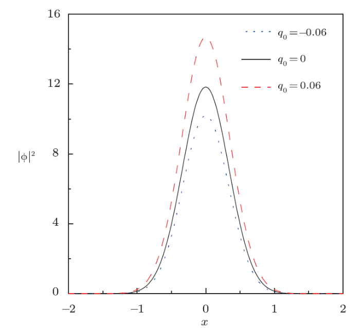 New window|Download| PPT slide
Fig.5Bell soliton density profiles versus $x$ obtained from variational analysis. Waveform for $\mu=-7.08$.
The behavior of the chemical potential $\mu$ versus the particle number $N$ for $q_{0}\leq0$ and the "ordinary" branch of $q_{0}>0$ are plotted in Fig. 2. It is shown that for a small $N$, the nonlinear eigenvalue $\mu$ matches very well with different $q_{0}$. However, tending to diverge as the particle number is increased. For a relative bigger $N$: with the positive quantum fluctuation (red-dashed line in Fig. 2) can enlarge the chemical potential $\mu$ compared with without quantum fluctuation (black-solid line in Fig. 2); the negative quantum fluctuation can reduce the chemical potential (blue dotted-line in Fig. 2). From Fig. 3, we can see the behavior of $\omega_{b}$ is similar. For small $N$, the effect of the quantum fluctuation on beam width can be negligible. Following the particle norm $N$ becomes larger, the effect of quantum fluctuation on $\omega_{b}$ is obvious.
In Figs. 4(a) and 4(b), it is shown the relationship between the chemical potential $\mu$ and width $\omega_{b}$ versus the particle number $N$ for the "extra ordinary" branch with $q_{0}>0$. The very localized soliton density profile is plotted in Fig. 4(c), the corresponding parameter is marked in Figs. 4(a) and 4(b). It is clearly shown that in this "extra ordinary" branch, following the increase of $N$, the chemical potential $\mu$ is growing nonlinear with $N$. However, the soliton's width is increasing approximately linearly with the increasing of $N$. And the corresponding robust soliton contains much larger $N$ as clearly shown in Fig. 4(c).
Note that stability of the localized modes in nonlinear system is a very important issue. In this section, we shall focus on the stability of $\mathcal{PT}$-symmetric solitons. The Vakhitov-Kolokolov (VK) stability condition ensures the stability of solitons for the 1D local GP equation.[35] The VK condition determines the stability of the solitons based on the sign of particle number versus chemical potential graph for bright solitons. If $\rm d N/\rm d\mu$ is positive, then the corresponding soliton is stable, otherwise, the soliton is unstable. Recently, the VK condition can also be extended to nonlinear Schr?dinger equations in complex external potentials to predict the domain of stability.[36-38] For the cases of $q_{0}\leq0$ or the "ordinary" branch as show in Fig. 2, it is clearly shown that $\rm d N/\rm d\mu$ is always negative, so the corresponding soliton is unstable. However, as shown in Fig. 4(a), with the help of positive quantum fluctuation $q_{0}$. For the "extra ordinary" branch solutions, where $\rm d N/\rm d\mu$ is always positive. Though the Vakhitov-Kolokolov (VK) stability condition, we can get conclusion that the soliton belonging to the "extra ordinary" branch for $q_{0}>0$ is always stable. Physically, due to the competition between attractive two-body interactions and positive quantum fluctuations, the repulsive force induced from quantum fluctuations can arrest the collapse and stabilize the system. A moderate quantum fluctuation can survive a robust bright soliton, but a larger positive quantum fluctuation can destroy a bright soliton.
5 Conclusion
In this work, we analyze the existence and stability of localized states of BEC with quantum fluctuations trapped in a $\mathcal{PT}$-symmetric potential. Within the mean-filed framework, we find that the quantum fluctuations can dramatically influence the $\mathcal{PT}$-soliton state in BEC. That means the quantum fluctuation can influence the $\mathcal{PT}$-symmetric soliton's profile, chemical potential and width. Most importantly, it is shown that with the help of positive quantum fluctuation, a robust stable $\mathcal{PT}$-symmetric bright soliton which contains much large particle norms will be found. Our results may be feasible experimentally, where the real part of the PT-symmetric potential is a simple Gaussian-shaped potential, which is easily achieved.[39] To implement imaginary part which accounts for gain-loss mechanisms, a pumping scheme can be exploited as well as optical dipole traps,[40] but the loss mechanisms can be implemented shining the BEC with electron beams.[41] And the strength of two-body interaction and quantum fluctuations can be tuned using Feshbach resonance.[42]Reference By original order
By published year
By cited within times
By Impact factor
[Cited within: 1]
[Cited within: 1]
[Cited within: 1]
[Cited within: 1]
[Cited within: 1]
[Cited within: 1]
[Cited within: 1]
[Cited within: 1]
[Cited within: 1]
[Cited within: 1]
[Cited within: 1]
[Cited within: 1]
[Cited within: 1]
[Cited within: 1]
[Cited within: 1]
[Cited within: 1]
[Cited within: 1]
[Cited within: 2]
[Cited within: 1]
[Cited within: 1]
[Cited within: 1]
[Cited within: 1]
[Cited within: 1]
[Cited within: 1]
[Cited within: 2]
[Cited within: 1]
[Cited within: 1]
[Cited within: 1]
[Cited within: 1]
[Cited within: 1]
[Cited within: 1]
[Cited within: 1]
[Cited within: 1]
[Cited within: 1]
[Cited within: 1]
[Cited within: 1]
[Cited within: 1]
