 ,?Department of Physics, Beijing Normal University, Beijing 100875, China
Corresponding authors: ?E-mail:
Received:2018-12-11Online:2019-07-1
| Fund supported: |

Abstract
KeywordsЃК
PDF (2622KB)MetadataMetricsRelated articlesExportEndNote|Ris|BibtexFavorite
Cite this article
Zhong Wang. Heisenberg-Type Quantum Steering by Continuous Weak Measurement in Circuit QED *. [J], 2019, 71(7): 798-806 doi:10.1088/0253-6102/71/7/798
1 Introduction
With further understanding of quantum nonlocality, quantum steering, a former casual theoretical concept, has attracted renewed attentions in the past decade.[1-2] Unlike the previously widely discussed description on quantum entanglement such as the density matrix inseparability and Bell nonlocality, quantum steering focuses on the state of local subsystem under the condition of measuring another distant subsystem. In the hierarchy of quantum nonlocality, steering lies between inseparability and Bell nonlocality with unique asymmetric properties.An attractive research field on quantum steering is its verification and quantification.[3-8] Steering inequality, proposed as an experimental criterion analogous to Bell inequality,[3] is utilized in various systems, including optomechanics,[9-13] Bose-Einstein condensates[14-16] and photons.[17-19] The studies in these systems shed light on the unique prosperities on quantum steering, as well as promote its practical applications such as high precision measurement[20] and quantum information processing.[21] Furthermore, plenty of experiments on steering are also conducted, for instance, experimental realization of the criteria,[22-24] steering with Bell local state,[25] one-way steering,[26-27] loophole free steering,[28-30] one-side device independent quantum key distribution.[31] However, These experiments are mostly limited in photon systems.
As a state-of-art experimental setup, the circuit quantum electro-dynamics (QED) system is not only a promising scheme in quantum information processing, but also a fascinating platform in exhibiting unusual quantum phenomena, such as the preparation of Schr?dinger's cat state,[32] the violation of Bell inequality,[33] and Leggett-Garg inequality.[34] For now, however there is still an absence of research on quantum steering conducted on a circuit QED system. In this work, we scrutinize the steering of the qubit state by continuous weak measurement on the cavity field and obtain a set of multiplicative steering inequalities based on the Heisenberg uncertainty principle. Unlike the position-momentum uncertainty relation in optomechanics, BEC and photon systems, there are three non-commutative components in the spin angular momentum of a qubit. We find that not every non-commutation relation can derive a usable steering inequality and then we analyze the reason. Furthermore, we discuss some important conditions of violating the steering inequality, including measurement strength, measurement method, and detector efficiency.
The rest of this paper is organized as follows. In Sec. 2 we briefly introduce the circuit QED system and the continuous weak measurement scheme in it. In Sec. 3, on the foundation of introducing the concept of steering, we get a set of multiplicative steering inequality and find that not every inequality can work as a criterion. In Sec. 4 we give an explanation and discuss several conditions for steering. We present a brief summary in Sec. 5.
2 Continuous Weak Measurement in Circuit QED System
A circuit QED setup consists of a one-dimensional superconducting transmission line and an artificial atom made of superconducting Josephson junctions. The transmission line driven by alternating-current (AC) voltage is treated as a harmonic oscillating cavity and the artificial atom is treated as a qubit. The Hamiltonian of the entire system is described by the Jaynes-Cummings (JC) modelwhere $\omega_q$ is the intrinsic frequency of the qubit, $\omega_r$ the frequency of the cavity field, $g$ the coupling strength between the cavity and the qubit, $\sigma^+$($a^\dagger$) and $\sigma^-$($a$) the raising and lowering operator of the qubit(cavity), respectively. $\mathcal{E} = \epsilon_m ({\rm e}^{-{\rm i}\omega_mt} + {\rm c.c.})$, in which $\epsilon_m$ is the driving strength and $\omega_m$ the driving frequency. A circuit QED system is usually measured in the dispersive regime, i.e. $\Delta \gg g$, in which $\Delta=|\omega_r-\omega_q|$ is the detuning between $\omega_r$ and $\omega_q$. Under this approximation, an effective Hamiltonian can be derived through unity transformation as
where $\tilde{\omega}=\omega_q+\chi$ and $\Delta_r=\omega_r-\omega_m$. $\chi=g^2/\Delta$ is the dispersive coupling strength between the cavity field and the qubit. Under the influence of the coupling term $\chi a^\dagger a \sigma_z$, the cavity field has a frequency shift depending on the qubit state. Thus the information of the qubit state can be gained by detecting the output cavity field.
The cavity field is usually detected through homodyne detection. System state at time $t$ without additional decay can be written as $|\Psi(t)\rangle=c_e(t) |e\rangle \otimes |\tilde{\alpha}_e(t)\rangle + c_g(t) |g\rangle \otimes |\tilde{\alpha}_g(t)\rangle$, in which $|\tilde{\alpha}_e(t)\rangle$ and $|\tilde{\alpha}_g(t)\rangle$ are stochastic coherent cavity states corresponding to the excited and ground state of the qubit $|e\rangle$ and $|g\rangle$, respectively. It is difficult to solve the exact cavity field states, but we can use their ensemble average instead and it is a good approximation.[35] The evolution equation of the approximated cavity field is
where $\kappa$ is the cavity photon leaking rate inversely proportional to the cavity Q-factor.
In circuit QED system, continuous weak measurement such as the homodyne detection is usually described by the quantum trajectory equation (QTE). When considering the steering of the qubit by the cavity field, we do not need to know the cavity field state (the rationale will be explained there-in-after), so it is possible to use the polaron transformation to eliminate the degrees of freedom (DOF) of the cavity field and obtain an effective QTE with only the qubit DOF.[36] The advantage of the effective QTE approach is that, as a harmonic oscillator, there are infinitely many cavity field energy levels, which make calculation very difficult. By omitting these additional DOF from consideration the calculation can be greatly simplified. Under a continuous homodyne measurement, the evolution of the qubit density matrix is
where $\omega_{\rm ac}=\omega_q+\chi+B(t)$ is the effective frequency of the qubit with AC Stark effect, in which $B(t) = 2\chi \textrm{Re}[\alpha_g(t)\alpha_e^*(t)]$. For an arbitrary operator $c$, the Lindblad superoperator is $\mathcal{D}[c]\rho=c \rho c^\dagger-({1}/{2})\{c^\dagger c,\rho\}$ and the measurement superoperator $\mathcal{M}[c]\rho=({1}/{2})\{(c-\langle c \rangle),\rho\}$. $\Gamma_{\rm ci}$ is the rate of extracting information from the qubit, i.e., the "spooky" back-action caused by entanglement. $\Gamma_{\rm ba}$ is the "realistic" back-action caused by the AC Stark effect.
where $\eta$ is the detector efficiency, $\varphi$ is the local oscillator (LO) phase of homodyne measurement and $\beta(t) = \alpha_e(t)-\alpha_g(t) = |\beta|{\rm e}^{\rm i\theta_\beta}$. The overall measurement rate is $\Gamma_m=(\Gamma_{\rm ba}+\Gamma_{\rm ci})/\eta=\kappa|\beta(t)|^2$, and the measurement strength can be characterized as $\Gamma_m t$. The overall qubit decay rate is $\Gamma_d = 2\chi \textrm{Im}[\alpha_g(t)\alpha_e^*(t)]$, which gives a limit to the upper bound of $\Gamma_m$. Both $\Gamma_m$ and $\Gamma_d$ are determined by the system parameters $\chi$, $\kappa$, and $\epsilon_m$. When the system parameters are specified, the measurement strength is proportional to measurement time $t$. Moreover, after the system evolutes into steady state, there is $\Gamma_d=\Gamma_m/2$, thus the quantum measurement efficiency can be expressed as $\eta=(\Gamma_{\rm ci}+\Gamma_{\rm ba})/2\Gamma_d$.
The output current of the homodyne measurement is
in which $\xi(t)$ is Gaussian white noise satisfying $E[\xi(t)]=0$ and $E[\xi(t)\xi(t')]=\delta(t-t')$. It reflects the randomness of quantum measurement. Under homodyne detection, the weakly measured qubit evolves gradually and stochastically.
3 Quantum Steering and Multiplicative Criteria in Circuit QED System
Here we briefly introduce the concept of quantum steering, then derive a set of multiplicative steering inequalities based on the Heisenberg uncertainty relation as criteria for experiments in the circuit QED system.Firstly, we review two frequently utilized viewpoints in describing entanglement, i.e., the inseparability of density matrix and Bell nonlocality. For a pair of particles separated in space, inseparability means that the total density matrix cannot be decomposed into the sum of the direct product of each particle's density matrix. It focuses on the quantum state of the system. Bell nonlocality means that the correlation of measurement results of each particle can exceed the upper bound predicted by a local hidden variable (LHV) theory. It focuses on the measurement results as c-numbers. For pure states, these two viewpoints are equivalent. However for mixed states, Werner proved in 1989 that the latter is a subset of the former.[37]
Therefore a natural but long neglected question is, how to describe the measurement result of particle $A$ and the state of particle $B$? There was no answer to this question until 2007, when Wiseman et al. formulized the effect on particle $B$ caused by measurement on particle $A$ and named it as steering, a word first proposed by Schr?dinger in 1935.[1-2] For a pair of entangled particles $A$ and $B$, the corresponding state of particle $B$, when measuring the observable $\hat{A}$ of particle $A$ and obtaining a result $a$, is called the conditional state of $B$ (under the condition of result $a$). Considering an ensemble of $A$ and $B$ particle pairs, if we obtain different conditional states of $B$ when measuring different observables of $A$, can we confirm that the measurement of $A$ has affected the state of $B$? For particles in mixed states, the answer is no. Because a possible explanation is that there is a set of local hidden states (LHS) of $B$ and the differences between conditional states come from different combinations of these LHS. With the LHS set $\{\rho_\lambda\}$, the conditional state of $B$ under the condition of obtaining result $a$ when measuring $\hat{A}$ could be written as
where $P(\lambda|a)$ is a pre-existed probability which is independent of measurement. In this way, different conditional states are made up only from different combinations of LHS without any nonlocal effect on the very state of $B$, i.e., without any steering.
To determine whether the conditional states of particle $B$ are steered by the measurements on $A$, or just follow some kind of LHS model, we need a criterion. As with the Bell inequality for the LHV model, we can use a steering inequality to check the LHS model. In optomechanics, BEC systems and photon systems, a multiplicative steering inequality can be derived from the position-momentum uncertainty relation $\Delta x\Delta p \ge 1/2$. However in a circuit QED system, there are three non-commutative observables and the measurement methods are quite different, so the situation becomes relatively more complex. We next investigate this issue.
For the Pauli operators of a qubit, there is commutation relation
in which $i$, $j$, and $k$ are cycles of $x$, $y$, and $z$, respectively. Then for arbitrary state, there exists the Heisenberg uncertainty relation
In circuit QED system, a steering task could be schemed as follows: Prepare the system into an initial state and choose an LO phase $\varphi_m$ (corresponding measurement method noted as $m$). Measure the qubit continuously and weakly. Meanwhile, record the homodyne output current $I(t)$. At the end of the evolution, measure a qubit observable $\sigma_i$ projectively and obtain the result $s=\pm1$. Repeat the above procedure many times. Then we can obtain the conditional absolute value $|\langle\sigma_i\rangle_I|$ and conditional variance $\Delta^2(\sigma_i|I)$ of observable $\sigma_i$ under condition $I(t)$. There is no two identical stochastic currents. However, technically we can pick out current close enough to instead approximately. For a specific measurement result $I(t)$, the conditional variance and absolute value are
where $s_I=\sum_s P(s|I)s$ is the conditional average.
Taking an average over all currents under the measurement method $m$, we can obtain the conditional absolute value $|\sigma_i^m|$ and variance $\Delta^2\sigma_i^m$ under the condition $\varphi_m$. For observable $\sigma_i$ and measurement method $m$, we have
in which $\Delta^2\sigma_i^m$ is the conditional variance of observable $\sigma_i$ averaged over all results $I(t)$ under measurement method $m$, and $|\sigma_i^m|$ is the conditional absolute value under the same condition.
It is noteworthy that in the above procedures, the measurement results are only a mark with which to classify the conditional states. Their exact values do not affect the judgement of the LHS model. Thus it is reasonable to eliminate the cavity field DOF in QTE as we did in Sec. 2. This is the asymmetry that makes quantum steering different from conventional density matrix inseparability and Bell nonlocality.
Through some simple derivations (see the Appendix), we can obtain a multiplicative steering inequality in circuit QED system
This is similar to the Heisenberg uncertainty relation in form, but different in intrinsic physical meaning. We then define a steering parameter $S_{ijk}^{mnl}$ as
where $i$, $j$, $k$ are cycles of $x$, $y$, $z$ and $m$, $n$, $l$ are labels of measurement methods. By comparing the steering parameter with 0, i.e., checking the violation of steering inequality, we can rule out LHS models of the qubit.
Consider two frequently used LO phases $\varphi_1=0$ and $\varphi_2=\pi/2$. For 3 subscripts corresponding to $\sigma_x$, $\sigma_y$, $\sigma_z$ and 2 superscripts corresponding to $\varphi_1$, $\varphi_2$ in steering parameter $S^{mnl}_{ijk}$, there are 18 different combinations. We find through simulation that not every steering parameter can be used to show the violation of steering inequality. This is different from the widely discussed position-momentum type steering inequalities in other systems. In fact, there are only 9 different combinations can be used to show steering; see Table 1.
Table 1
Table 1Steering parameters are corresponding to different observables and different measurement methods. ЁАYЁБ and ЁАNЁБ indicates whether a steering parameter can be used to show the violation of the steering inequality or not.
 |
New window|CSV
4 Results and Discussion on Steering Conditions
By theoretically and numerically analyzing the evolution of qubit under continuous weak measurement, we explain the reason behind which specified steering parameters can be used to show the violation of steering inequality. We also discuss some conditions that may need to be considered in experiment, including measurement strength of the qubit, measurement method (characterized by the LO phase) and detector efficiency.For simplicity, we set the initial state of the system as $(|e\rangle+|g\rangle) \otimes |\alpha\rangle$ (not normalized) and consider the situation without additional decay.
When the LO phase $\varphi=0$, it has $\Gamma_{\rm ci}=\Gamma_m$ and $\Gamma_{\rm ba}=0$, which means the qubit state information is gradually obtained through continuous weak measurement. As the information is obtained, the qubit state gradually and stochastically collapse to either $|e\rangle$ or $|g\rangle$. Without loss of generality, we assume the qubit final state is $|g\rangle$. When measuring $\sigma_x$ we have $P(x=+1)=P(x=-1)=1/2$, which means it is completely uncertain. Thus $|\langle \sigma_x \rangle_I|$ reaches a minimum of 0 and $\Delta(\sigma_x|I)$ reaches a maximum of 1. The same argument applies for $\sigma_y$. When measuring $\sigma_z$ we have $P(z=-1)=1$. Thus $|\langle \sigma_z \rangle_I|$ reaches a maximum of 1 and $\Delta(\sigma_z|I)$ reaches a minimum of 0.
When $\varphi=\pi/2$, $\Gamma_{\rm ci}=0$, and $\Gamma_{\rm ba}=\Gamma_m$, the measurement does not obtain information of the qubit state, but only drive the qubit coherently through AC stark effect. The $\sigma_x$ and $\sigma_y$ components oscillate stochastically and the $\sigma_z$ component keeps unchanged because no information is extracted. For stochastically oscillation, the variance and absolute value will evolute into a steady state. Through numerical simulation we find that it is a value decided by system parameters between 0 and 1. For $\sigma_z$, $P(z=+1)=P(z=-1)=1/2$, thus $\Delta(\sigma_z|I)$ stays at a maximum of 1 and $|\langle \sigma_z \rangle_I|$ stays as a minimum of 0.
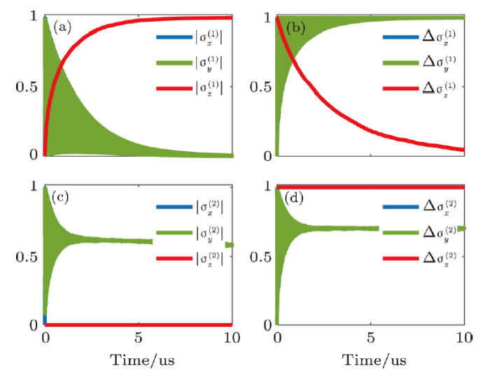
According to the above analysis of the conditional values under specific measurement result $I(t)$, we can have an understanding on each term in steering parameter by averaging over all $I(t)$ with $P(I|m)$. The evolution of each term is shown in Fig. 1. We can find that $|\sigma_x^{(1)}|$ and $|\sigma_y^{(1)}|$ decrease to a minimum of 0 with oscillating, in which the frequency is very high because of large $\omega_q$ which is usually at GHz in practical experiment. $|\sigma_z^{(1)}|$ increases to a maximum of 1. $\Delta\sigma_x^{(1)}$ and $\Delta\sigma_y^{(1)}$ increase to a maximum of 1 with oscillating while $\Delta\sigma_z^{(1)}$ decreases to a minimum of 0. $|\sigma_x^{(2)}|$ and $|\sigma_y^{(2)}|$ evolve into steady value while $\Delta\sigma_x^{(2)}$ stays at 0. $\Delta\sigma_x^{(2)}$ and $\Delta\sigma_y^{(2)}$ evolve into steady value while $\Delta\sigma_z^{(2)}$ keeps in 1. The numerical evolution under specified $m$ agrees with our analysis above under specific $I(t)$.
Fig. 1
 New window|Download| PPT slide
Fig. 1(Color online) The evolution of terms in the steering parameter. System parameters are $\chi=0.1$ MHz, $\kappa=100$ MHz, $\epsilon_m=400$ MHz, $\Delta=2.5$ GHz. (a) $|\sigma_i^{(1)}|$ when $\varphi=0$. (b) $\Delta\sigma_i^{(1)}$ when $\varphi=0$. (c) $|\sigma_i^{(2)}|$ when $\varphi=\pi/2$. (d) $\Delta\sigma_i^{(2)}$ when $\varphi=\pi/2$. In all sub-figures blue, green, and red represents $x$, $y$, and $z$ respectively.
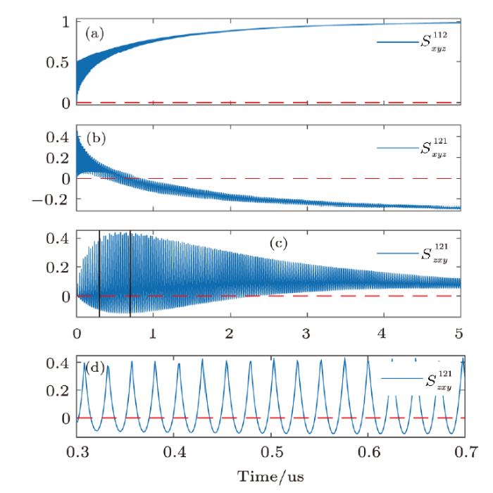
To violate the steering inequality, small $\Delta\sigma_i^m$ and large $|\sigma_k^l|$ should be chosen to make the steering parameter $S^{mnl}_{ijk}$ less than 0. Three typical combinations of measurement methods and observables are presented in Fig. 2. Fig.2(a) $S^{112}_{xyz}$ in Fig. 2(a) is an instance that can not violate the steering inequality. According to the above discussion, we know that $\Delta\sigma_x^{(1)}$ and $\Delta\sigma_y^{(1)}$ gradually increase to 1 and $|\sigma_z^{(2)}|$ stays at 0. Thus $S^{112}_{xyz}$ increases to 1 and will never be less than 0. Fig.2(b) Figure 2(b) shows $S^{121}_{xyz}$, which is an instance of violating the inequality. In this case, $\Delta\sigma_x^{(1)}$ gradually increases to 1, $\Delta\sigma_y^{(2)}$ oscillates into a finite steady value between 0 and 1, and $|\sigma_z^{(1)}|$ stays at 1. Thus after a period of evolution, the entire parameter value is less than 0 before the system completely collapses. Fig.2(c) $S^{121}_{zxy}$ in Fig. 2(c) is more interesting. In the stage of establishing steady state, $\Delta\sigma_z^{(1)}$ keeps at 1, $\Delta\sigma_x^{(2)}$ and $|\sigma_y^{(1)}|$ both oscillate. A numerical "interference" between $\Delta\sigma_x^{(2)}$ and $|\sigma_y^{(1)}|$ will lead to a large oscillation amplitude of $S^{121}_{zxy}$. Thus when the measurement strength is small, the violation of steering inequality can be shown. However, it disappears after the steady state is established. This is a direct example which shows the effect of weak measurement strength in multiplicative steering inequality. Fig.2(d) To see this more clear, $S^{121}_{zxy}$ on the time period from 300 ns to 700 ns is plotted in Fig. 2(d).
Fig. 2
 New window|Download| PPT slide
Fig. 2(Color online) Evolution of several typical steering parameters $S_{ijk}^{mnl}$. Subscripts for observables $x$, $y$ and $z$, superscripts for measurement methods $\varphi_1$ and $\varphi_2$. (a) $S^{112}_{xyz}$ cannot violate the steering inequality. (b) $S^{121}_{xyz}$ violates the steering inequalities after a period of evolution. The minimum is $-0.31$. (c) $S^{121}_{zxy}$ violates the inequality only when oscillating to valleys before getting into steady state. The minimum is $-0.11$. Evolution times in (a), (b) and (c) are from 0 to 5 $\mu$s. (d) $S^{121}_{zxy}$ from 0.3 $\mu$s to 0.7 $\mu$s, i.e., the vertical black lines in (c), in which the steering inequality is violated intermittently. System parameters are the same as
The oscillations in Figs. 1 and 2 are originated from the AC Stark shift of the qubit energy caused by the dispersive homodyne readout. To demonstrate the violation of the steering inequality in experiment, one only needs to choose a specific time, i.e., a proper measurement strength. Moreover, the measurement results is Gaussian stochastic currents and the oscillations do not directly appear in the measurement results. In an experiment, if a specified current $I(t)$ is obtained, and the system initial state and system parameters are already known, one could estimate the system state $\rho(t)$ and its evolution trajectory, then calculate the steering parameter. Furthermore, it is worth noting that unlike the Bell inequality of LHV model, the violation of a steering inequality is only a sufficient condition rather than a necessary condition for ruling out LHS model. However even a sufficient criterion is valuable in practical applications, for instance, in one side device independent QKD.[31] In fact, it is an attractive field in recent years to search more universal and tighter steering criteria.[38-39]
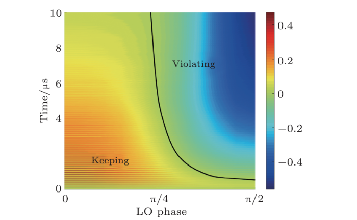
The analysis above is based on two typical measurement methods $\varphi=0$ and $\pi/2$. In circuit QED system, the LO phase of a homodyne measurement can be adjusted continuously to realize different measurement methods. We consider a steering parameter $S^{mnl}_{yzx}$ in which LO phase corresponding to $|\sigma_x^{(l)}|$ is fixed on $\pi/2$ while LO phase corresponding to $\Delta \sigma_y^{(m)}$ and $\Delta\sigma_z^{(n)}$ change from $0$ to $\pi/2$ continuously. When the phase difference $\Delta\varphi=0$, it degenerates into the trivial situation with same measurement method and cannot show any steering. When the phase difference $\Delta\varphi=\pi/2$, it is the situation with $\varphi_1$ and $\varphi_2$ discussed above. For $\Delta\varphi$ between 0 and $\pi/2$, noticing that $\Gamma_{\rm ba}$ and $\Gamma_{\rm ci}$ are monotonic functions of $\varphi$, we can infer that $S^{mnl}_{yzx}$ is between the two situations of $\Delta\varphi=0$ and $\pi/2$. The surface plot in Fig. 3 confirms our analysis. It can be seen when the measurement is very weak, there is no proper $\Delta\varphi$ that can show steering. As the measurement becomes stronger, the critical $\Delta\varphi$ becomes smaller. A violation bound is plotted to show this directly. Generally speaking, showing steering requires a long measurement time and a large phase difference.
Fig. 3
 New window|Download| PPT slide
Fig. 3(Color online) Steering parameter $S_{mnl}^{yzx}$ versus measurement time $t$ and LO phse difference $\Delta\varphi$, in which $\varphi_m$, $\varphi_n$ change from 0 to $\pi/2$ and $\varphi_l=\pi/2$. The black line is the bound between keeping and violating inequality.
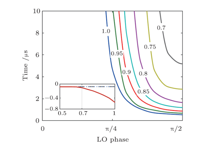
In practical circuit QED system, the detector efficiency $\eta$ is always an important restriction and be treated as an indicator of the "detector dependency" of a quantum system.[40-41] We now discuss the effect on steering by a non-ideal detector. With $\eta$ changing from 1.0 to 0.5, the violation bounds are plotted in Fig. 4. As the detector efficiency decreases, the violation region narrows. When the efficiency is less than 0.7, the violation region disappears and we cannot check whether steering exists through multiplicative inequality any more. To see this more clearly, we show the minimum steering parameter versus efficiency in the inset of Fig. 4. Comparing with an ideal detector, low detector efficiency will bring about more mixed components in the system state. Steering is a quantum phenomenon just like the density matrix inseparability and Bell nonlocality, while the mixed state is described by classical probability. Thus it is not surprising that low detector efficiency will depress quantum steering. Daryanoosh et al. proved that for all processes described by QTE, the lowest efficiency to show steering is 0.5. Our results do not violate their prediction.[41] We also notice that, in the state-of-the-art experimental setup, a quantum efficiency of $\eta=0.67$ is reported,[42] which almost satisfies the steering requirement.
Fig. 4
 New window|Download| PPT slide
Fig. 4(Color online) Bound of $S^{mnl}_{yzx}$ under different detector efficiencies $\eta$, which vary from 0.5 to 1.0. When $\eta<0.7$, the violation region disappears. Inset indicates the minimum of $S^{mnl}_{yzx}$ under different efficiencies.
5 Summary
In summary, on the foundation of introducing measurement in circuit QED system and EPR steering, we obtained a set of multiplicative steering inequalities as criteria for the steering of a qubit by the measurement of the cavity field. Through simulation, we found that unlike in other widely studied systems, there are only several specified types of steering inequality can be used to show steering, and we also analyzed the reason for this. We then discussed several conditions that may affect steering in practical experiment, including measurement strength, method and detector efficiency. By adjusting the LO phase continuously, we found that for continuous weak measurement, a large LO difference is helpful. High detector efficiency also has benefits and there exists a lower measurement efficiency bound of steering.Our work may be helpful to EPR steering experiments in circuit QED system. For now, steering experiments in the photon system mostly focus on projective measurement, while the technique of weak measurement of photons has already been applied to the measurement of photon states.[43] This work also sheds light on the steering with weak measurement The comparison and connection of steering with density matrix inseparability and Bell nonlocality in circuit QED system is also an interesting potential work. The preliminary discussion in this work may also be generalized to a multi-qubit circuit QED system.
Appendix A: Derivation of the Multiplicative Steering Inequality
For circuit QED system with the LO phase $\varphi_m$, the output current $I$, the qubit observable $\sigma_i$, and the qubit measurement result $s$, the conditional average of $s$ under the current $I$ is
where $P(s|I)$ is the probability of getting $s$ under condition of getting $I$, and the conditional probabilities there-in-after are in similar forms. The conditional variance is
When measuring the cavity field, if there exists an LHS model for the qubit, the conditional qubit state under $I$ can be written as
where the subscript $q$ in $\rho_{(q|I)}$ means "qubit". According to the quantum measurement theory,
where $M_s$ is the measurement operator of obtaining result $s$ when measuring the qubit. For arbitrary $a$ and $b$, according to probability theory we have the following relation:
Inserting Eq. (A3) into Eq. (A5) we obtain
Defining the variance of $\sigma_i$ under measurement method $m$ as $\Delta^2 \sigma_{i}^{m}=\sum_I P(I|m)\Delta^2(\sigma_i|I)$, considering Eq. (A6) we obtain
For a quantum state $\rho_\lambda$, the Heisenberg uncertainty relation is
Here we use Cauchy-Schwarz inequality: $|\vec{u}|\cdot|\vec{v}| \ge |\vec{u}\cdot\vec{v}|$, let $\vec{u}$ and $\vec{v}$ be
Noticing that $\lambda$ is independent from measurement method, i.e. $P(\lambda|m)=P(\lambda|n)=P(\lambda)$, then we obtain
Defining $|\sigma_{k}^{l}|=\sum_I P(I|l)|\langle \sigma_k\rangle_I|$, with the following Triangle Inequality
we obtain
Insert Eq. (A12) into Eq. (A10) we finally have
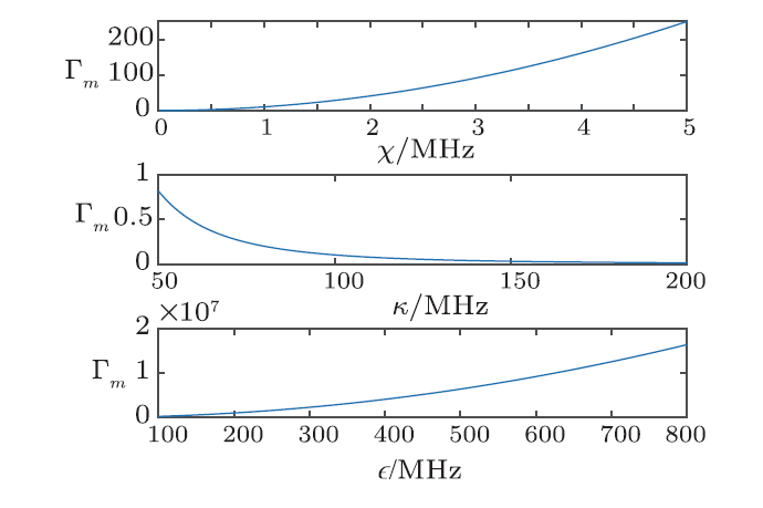
The system parameters $\chi$, $\kappa$, and $\epsilon_m$ determine the measurement rate $\Gamma_m$, as well as the qubit evolution, i.e., they affect the qubit indirectly through the measurement rate. When $\chi$ and $\epsilon_m$ increase, the coupling between cavity field and qubit, and the cavity driving amplitude is strong, which lead to a large $\Gamma_m$. However when $\kappa$ increases, $\Gamma_m$ decreases. It is because even though the photon leaking rate is large, the cavity field difference becomes small. Thus the information carried out by the photons in unit time decreases. For more results with different system parameters are given below. The multiplicative steering inequality is valid in a typical range of experimental system parameters.
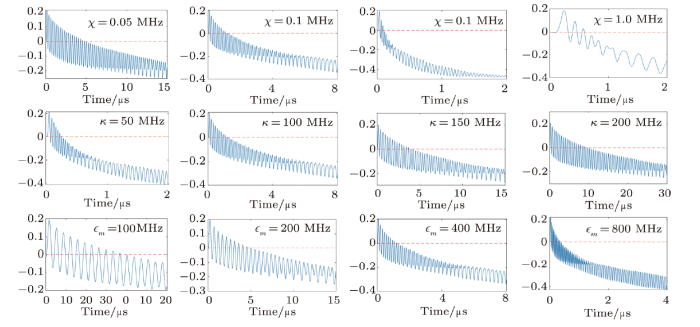
The dependence of $\Gamma_m$ under steady state and the system parameters are plotted in Fig. 5. More over, steering parameter $S_{xyz}^{121}$ under $\chi=(0.05$, $0.1$, $0.5$, $1.0$) MHz, $\kappa=(50$, $100$, $150$, $200$) MHz, and $\epsilon_m=(100$, $200$, $400$, $800$) MHz are plotted in Fig. 6. It can be seen that our result is valid in a typical range of experimental system parameters.
Fig. 5
 New window|Download| PPT slide
Fig. 5(Color online) $\Gamma_m$ vs $\chi$, $\kappa$ and $\epsilon_m$.
Fig. 6
 New window|Download| PPT slide
Fig. 6(Color online) $S_{xyz}^{121}$ with different parameters.
Reference By original order
By published year
By cited within times
By Impact factor
[Cited within: 2]
[Cited within: 2]
[Cited within: 2]
[Cited within: 1]
[Cited within: 1]
[Cited within: 1]
[Cited within: 1]
[Cited within: 1]
[Cited within: 1]
[Cited within: 1]
[Cited within: 1]
[Cited within: 1]
[Cited within: 1]
[Cited within: 1]
[Cited within: 1]
[Cited within: 1]
[Cited within: 1]
[Cited within: 1]
[Cited within: 1]
[Cited within: 2]
[Cited within: 1]
[Cited within: 1]
[Cited within: 1]
[Cited within: 1]
[Cited within: 1]
[Cited within: 1]
[Cited within: 1]
[Cited within: 1]
[Cited within: 1]
[Cited within: 2]
[Cited within: 1]
[Cited within: 1]
