<script type="text/javascript" src="https://cdn.bootcss.com/mathjax/2.7.2-beta.0/MathJax.js?config=TeX-AMS-MML_HTMLorMML"></script> <script type='text/x-mathjax-config'> MathJax.Hub.Config({ tex2jax: {inlineMath: [['$','$'], ['\\(','\\)']]}, "HTML-CSS": { scale: 100, minScaleAdjust: 100, mtextFontInherit: true, } }); </script> Guifu ZHANG^1,,,
Jidong GAO²,
Muyun DU³

Corresponding author: Guifu ZHANG,guzhang1@ou.edu;

1.School of Meteorology, University of Oklahoma, Norman, OK 73072, USA
2.National Severe Storms Laboratory/NOAA, Norman, OK 73072, USA
3.Institute of Heavy Rain, CMA, Wuhan 430205, China
Manuscript received: 2020-08-24
Manuscript revised: 2020-11-06
Manuscript accepted: 2021-01-14
Abstract:Many weather radar networks in the world have now provided polarimetric radar data (PRD) that have the potential to improve our understanding of cloud and precipitation microphysics, and numerical weather prediction (NWP). To realize this potential, an accurate and efficient set of polarimetric observation operators are needed to simulate and assimilate the PRD with an NWP model for an accurate analysis of the model state variables. For this purpose, a set of parameterized observation operators are developed to simulate and assimilate polarimetric radar data from NWP model-predicted hydrometeor mixing ratios and number concentrations of rain, snow, hail, and graupel. The polarimetric radar variables are calculated based on the T-matrix calculation of wave scattering and integrations of the scattering weighted by the particle size distribution. The calculated polarimetric variables are then fitted to simple functions of water content and volume-weighted mean diameter of the hydrometeor particle size distribution. The parameterized PRD operators are applied to an ideal case and a real case predicted by the Weather Research and Forecasting (WRF) model to have simulated PRD, which are compared with existing operators and real observations to show their validity and applicability. The new PRD operators use less than one percent of the computing time of the old operators to complete the same simulations, making it efficient in PRD simulation and assimilation usage.
Keywords: forward operators,
polarimetric radar data,
data assimilation,
numerical weather prediction
摘要:现在，世界上许多天气雷达网都能提供偏振雷达数据（PRD），它们有可能增进我们对云和降水微物理的理解以及改进数值天气预报（NWP）。为了实现这一潜力，需要一套准确有效的偏振雷达观测算子，以便NWP模式能模拟和同化PRD，从而准确分析出模式状态变量。为此，我们开发了一组参数化观测算子，以根据NWP模型预测的水凝物混合比和雨，雪，冰雹和霰的数浓度来模拟和同化偏振雷达数据。偏振雷达变量是基于波散射的T矩阵方法以及由粒度分布加权积分计算得到。然后将计算出的偏振变量拟合为水含量和水凝颗粒粒径分布的体积加权平均直径的简单函数。将参数化的PRD前向算子应用于由天气研究和预报（WRF）模式预测的理想情况和实际案例来模拟PRD。并将其结果与现有的前向算子和实际观测值进行比较，以显示其有效性和适用性。新的PRD前向算子使用不到旧算子的计算时间的1%来完成相同的运算，从而使其在PRD模拟和同化使用中非常有效。
关键词:前向算子,
偏振雷达数据,
资料同化,
数值天气预报

HTML

--> --> -->

Many weather radar networks in the world have been upgraded with dual-polarization capability and provide polarimetric radar data (PRD) that have the potential to improve cloud microphysical parameterization and numerical weather prediction (NWP) (Zhang et al., 2019). PRD have been successfully used in severe weather observation/detection, hydrometeor classification (HC), and quantitative precipitation estimation (QPE) (Doviak and Zrni?, 1993; Doviak et al., 2000; Bringi and Chandrasekar, 2001; Zhang, 2016; Ryzhkov and Zrnic, 2019). Most of these applications are observational and empirical, which is not optimal because of the many assumptions that have to be made to facilitate an estimation/retrieval, and because the error effects have not been taken into account rigorously in the estimation/retrieval process. More importantly, PRD have not been successfully used to initialize NWP models for an improved quantitative precipitation forecast (QPF). Preliminary research is being conducted in this area, but it is still in its embryonic stages (Jung et al., 2008b; Li and Mecikalski, 2010; Posselt et al., 2015; Carlin et al., 2017; Li et al., 2017; Putnam et al., 2019).
One way to optimally use PRD is to assimilate PRD into NWP models to improve weather quantification and forecasts. This is an important goal for the radar meteorology and NWP communities because PRD contain rich information about clouds/precipitation microphysics: size, shape, orientation, and composition of hydrometeors, which allow for better understanding, representation, and parameterization of model microphysics and model initialization. However, even with PRD, the amount of independent information is limited and oftentimes less than that of model state variables. This is especially true for the double or multi-moment microphysics parameterization schemes, where there can be more than a dozen microphysical state variables (Ferrier, 1994; Milbrandt and Yau, 2005a, b; Morrison et al., 2005). Hence, NWP model physics constraints are still needed. Also, the PRD analysis/retrieval needs to be compatible with the NWP model so that the analysis can be used in model initialization to improve forecasts. To assimilate PRD in NWP models, a forward observation operator, also called a PRD simulator, is needed to establish the relation between model physics state variables and polarimetric radar variables.
So far, the radar reflectivity operators have been established mostly based on the 6th moment of raindrop size distribution (DSD) or hydrometeor particle size distribution (PSD) and used to simulate radar observations and to assimilate radar data (Smith et al., 1975; Ferrier et al., 1995; Sun, 2005; Gao and Stensrud, 2012; Pan et al., 2016). These reflectivity operators were developed based on the approximation of Rayleigh scattering by hydrometeors where the radar cross-section is proportional to the square of the particle volume (i.e., the 6th power of the diameter) and are valid only for small spherical particles. These operators are overly simplified, and do not provide polarimetric radar variables and cannot accurately represent polarimetric radar signatures of hydrometeors in the ice and mixture phases (e.g., snow/hail/graupel) nor the melting process when non-Rayleigh scattering (resonance effects) occurs or non-spherical particles are present.
Recently, PRD simulators have been developed based on the numerical integration of T-matrix calculations for wave scattering from hydrometeors (Waterman, 1965; Vivekanandan et al., 1991; Zhang et al., 2001; Jung et al 2008a, 2010; Ryzhkov et al., 2011); The computer code in the Fortran language for the PRD operators, documented in Jung et al. (2010), is posted on the University of Oklahoma website (http://arps.ou.edu/downloadpyDualPol.html). Scientists from Stony Brook University and Brookhaven National Laboratory also developed a Cloud Resolving Model Radar Simulator (CR-SIM) and made it available (http://radarscience.weebly.com/radar-simulators.html). Another operator, called the POLArimetric Radar Retrieval and Instrument Simulator (POLARRIS), was developed by the Colorado State University and NASA scientists (https://cloud.gsfc.nasa.gov/POLARRIS/) (Matsui et al., 2019). These PRD simulators are successful in generating realistic polarimetric signatures such as Z_DR arc, ρ_hv ring and so forth that have been observed (Kumjian and Ryzhkov, 2008). However, these simulators are used, for the most part, as a black-box by most NWP modelers, and it is difficult to understand what insights/information they could bring to understanding the physical states and processes they simulate and to make adjustments on NWP models based on these insights. Furthermore, the simulators are computationally expensive and difficult to use in data assimilation (DA), especially in variational assimilation where the first derivatives of the variables are needed as well. To have a successful DA of PRD, the PRD operator needs to be accurate, efficient, differentiable, and compatible with the model microphysical parameterization schemes. This motivates us to derive a set of parameterized PRD simulators to link NWP model state variables and radar variables for efficient DA use.
This paper is organized as follows. Section 2 provides the fundamentals concerning microphysics models and parameterization schemes about particle size, shape, orientation, and composition as well as their effects on polarimetric radar variables. Section 3 describes the procedure to derive parameterized polarimetric radar operators for rain, snow, hail, and graupel, including the function form and fitting coefficients. Section 4 shows the testing results with NWP model simulations for ideal and real cases. Section 5 concludes with a summary and discussion.

Single moment and double moment microphysics parameterization schemes are commonly used in NWP models (Lin et al., 1983; Ferrier, 1994; Milbrandt and Yau, 2005a, b; Morrison et al., 2005). In a single moment NWP model, hydrometeor mixing ratios, which are directly related to water contents, are the only prognostic variable for hydrometeor physics, from which all other integral parameters, including the number concentration and radar reflectivity, are represented. In a double moment microphysics scheme, both the number concentration and the hydrometeor mixing ratio are prognostic variables. Based on these variables, a two-parameter DSD/PSD is determined/represented, along with all other physics variables and microphysical processes. For a given two-parameter DSD/PSD model, the hydrometeor mixing ratio and the number concentration can be converted to a mass-weighted diameter and water content.
Let the DSD/PSD of hydrometeors be exponentially distributed, represented by
where D (mm) is the particle diameter, N₀ (m^?3 mm^?1) is the intercept parameter and $ \Lambda $ (mm^?1) is the slope parameter.
For a hydrometeor species x, a NWP model with a two-moment microphysics scheme usually predicts the number concentration (N_t,x) and mixing ratio (q_x) which is related to water content by W_x = ρ_aq_x, with ρ_a as the air density. Expressing the DSD/PSD parameters of Λ_x and N_0x in terms of the predicted variables, we have
where the hydrometeor particle density is ρ_x. Once the DSD/PSD parameters are found, all integral physical states/processes are ready to be calculated. Ignoring the truncation effects, the DSD/PSD moment is
and the mass/volume-weighted diameter ${D_{\rm{m}}}$ is also commonly used and can be defined using DSD/PSD moments as
We choose to parameterize radar variables in term of D_m,x (mm) and W_x=ρ_aq_x (g m^?3). In the case of a melting process, species such as melting snow, hail, and graupel, the hydrometeor particle density ρ_x (g cm^?3) is given as a function of the percentage of melting ${\gamma _x} = {q_{\rm{r}}}/({q_{\rm{r}}} + {q_x})$ (Jung et al., 2008a),
where ρ_dx is the density of dry snow, hail, or graupel, and ρ_w is the density of water. The shape and orientation of hydrometeor particles also follow the modeling and representation documented in Jung et al. (2008a), except for the mean axis ratio and standard deviation of the canting angles, which is described in the next section.

A dual-polarization weather radar measures reflectivity factor (also called reflectivity: Z or Z_H), Doppler radial velocity (v_r), spectrum width (σ_v), differential reflectivity (Z_DR), co-polar correlation coefficient (ρ_hv), and differential phase (?_DP) and/or a half of its range derivative – specific differential phase (K_DP). While radial velocity and spectrum width represent mean and random dynamic motion projected in the beam directions, the other four polarimetric measurements represent clouds/precipitation microphysics: size, shape, orientation, composition/density, temperature, and so forth. Next, we describe how the microphysical information is reflected in wave scattering and hydrometeor PSD.
The effective radar reflectivity measures the integrated radar scattering cross-section in a unit volume. After normalization, the radar reflectivity factor $ {Z}_{{\rm{h}},{\rm{v}}} $ ($ {{\rm{m}}{\rm{m}}}^{6}\;{{\rm{m}}}^{-3} $) is expressed by
where the equivalent diameter D is in mm, and N(D) ($ {{\rm{m}}}^{-3}\;{{\rm{m}}{\rm{m}}}^{-1} $) is the PSD, $ \lambda $ is the radar wavelength (mm), ${K_{\rm{w}}} = ({\varepsilon _{\rm{w}}} - 1)/({\varepsilon _{\rm{w}}} + 2)$ is the dielectric constant factor of water, and $ {s}_{{\rm{h}}{\rm{h}},{\rm{v}}{\rm{v}}}\left({\rm{\pi }},\;{{D}}\right) $ (mm) is the backscattering amplitude at the horizontal or vertical polarization.
In the Rayleigh scattering regime where particle sizes are spherical and much smaller than a wavelength [e.g., $ D<(\lambda /16)$ for raindrops], Eq. (8) reduces to ${Z_{{\rm{h,v}}}} \to (|{K_x}{|^2}/|{K_{\rm{w}}}{|^2}){Z_x}$ with the reflectivity factor for species x, and Z_x=M_6x is widely used in radar meteorology and NWP/DA communities (Smith et al., 1975, Ferrier, 1994). However, the above simplification is not always valid, especially for melting snow, hail, and graupel at S-band, and higher frequency bands such as C- and X-bands.
The reflectivity factor for horizontal polarization $ {Z}_{\rm{H}} $ represented in decibels (dBZ) is:
The differential reflectivity (dB), representing the difference in radar reflectivity between horizontal and vertical polarized waves, depends on the shape and orientation as well as composition of hydrometeors. It is defined as the ratio of reflectivity between the horizontal and vertical polarizations:
Specific differential phase (^o km^?1) is the phase difference between the horizontally and vertically polarized waves across a unit distance
where $ {\rm{s}}_{{\rm{h}}{\rm{h}},{\rm{v}}{\rm{v}}}\left(0,D\right) $ in (mm) is the forward scattering amplitude at the horizontal or vertical polarization, and Re(…) denotes the real part of the scattering amplitudes.
The co-polar correlation coefficient is the representation of the similarity between the horizontally and vertically polarized signals, whose reduction is mainly caused by the randomness of the differential scattering phase of the hydrometeors in the resolution volume, written as
In principle, polarimetric radar variables are readily calculated from Eqs. (8?12) with NWP model output through PSD and the scattering amplitudes, s_hh/s_vv, which can be calculated using the T-matrix method. This is done for the polarimetric radar operators released on-line (Jung et al., 2010, Matsui et al., 2019). In practice, however, this is neither convenient nor efficient for DA use which requires the operators to be differentiable for fast calculation. It would be more convenient if the operators can be represented directly by model state variables using a simple function form.
For rain, the polarimetric radar variables have recently been represented in mixing ratio and mass/volume-weighted diameter (Mahale et al., 2019). Raindrops are assumed to be spheroid with the axis ratio given by Eq. (2.16) in Zhang (2016). Using the T-matrix calculated scattering amplitudes, s_hh/s_vv, in Eqs. (8?12), polarimetric variables are calculated for a unit water content (W= ρ_aq_r =1 g m^?3) and a set of mass/volume-weighted mean diameters (D_m), with the exponentially distributed DSDs. The calculated radar variables are then fitted to polynomial functions of D_m, derived in Mahale et al. (2019), which are duplicated here:
where the units of W = ρ_aq_r are g m^?3 and q_r is the mixing ratio for rain. This allows for quick calculations of polarimetric radar variables from NWP model outputs (q_r, N_t). The reason for choosing this form for Eq. (13) is to reduce the number of terms/coefficients to simplify the calculation of reflectivity, which already requires the higher-order terms of D_m.
In the case of mixtures such as snow, hail, and graupel, the calculations and parameterizations are more complicated than those of rain because of the increased variability in density during the melting stage and irregular shape, as well as the orientation of the particles. Because most NWP models do not predict the density during the melting process, we estimate the percentage of melting from the relative rain mixing ratio and the density with Eq. (7). For a given species x, polarimetric radar variables are calculated for a set of the volume-weighted mean diameter at a given percentage of melting, and then parameterized as a function of the volume-weighted mean diameter (D_m) as follows
Since the fitting coefficients depend on the percentage of melting, the above calculation and fitting procedure is done for different percentages of melting (${\gamma _x}$). Then, the coefficients of the radar variables are further represented by a polynomial function of ${\gamma _x}$
For snow, the percentage of melting and the snow density is defined in Eq. (7) with ρ_dx = 0.1 g cm^?3 and ρ_w = 1.0 g cm^?3. The shape of snowflakes is assumed to be spheroid with an axis ratio of 0.7, changed from 0.75 which was used in Jung et al. (2008a). They are oriented at a mean angle of zero and standard deviation of 30 degrees, which is increased from the standard deviation of 20 degrees previously used. The purpose for these changes in shape and orientation of snowflakes is to allow a large dynamic range of ρ_hv and Z_DR. The calculated radar variables of snow for a unit snow water content (W_s = ρ_aq_s = 1 g m^?3) and the fitted curves are plotted as a function of the volume-weighted mean diameter for a variety of melting percentages. These are shown in Fig. 1. The fitting coefficients are provided in Table 1.
Figure1. Calculated (scattered points) and fitted (solid lines) polarimetric radar variables of snow as functions of the volume-weighted mean diameter for a variety of melting percentages: (a) reflectivity (Z_h, dBZ), (b) differential reflectivity (Z_dr, dB), (c) specific differential phase (K_DP, o km^?1), and (d) co-polar correlation coefficient (ρ_hv). The solid black lines for dry snow (lower) and wet snow (upper) in (a) are the results of reflectivity for Rayleigh scattering approximation.

		c0	c1	c2	c3
Zh	aZ0	0.0524	1.698	1.185	?2.063
	aZ1	?0.001886	?0.02846	?0.02812	?0.006190
	aZ2	?0.00004009	0.006846	?0.03071	0.04697
	aZ3	0.00000485	?0.0003777	0.001649	?0.002278
Zdr	ad0	1.018	0.8789	?0.0736	?0.2990
	ad1	0.001432	?0.02274	0.2280	?0.1841
	ad2	0.0004199	0.0000723	?0.001305	?0.002658
KDP	aK0	0.001180	0.1465	4.006	?3.356
	aK1	0.001650	?0.07655	0.3985	?0.2848
	aK2	?0.00007765	0.002322	?0.01327	0.006620
${\rho _{{\rm{hv}}}}$	${a_{\rho 0}}$	0.9975	?0.01015	?0.009316	0.001187
	${a_{\rho 1}}$	0.0001041	0.01452	?0.05034	0.02961
	${a_{\rho 2}}$	?0.0000137	?0.001039	0.002712	?0.001391

Table1. Fitted coefficients for snow at canting angle of 30 degrees.


Figure2. Same as Fig. 1, but for hail.


As shown in Fig. 1a, the reflectivity factor increases as the volume-weighted diameter and the melting percentage increase, which is to be expected because of the enhanced wave scattering due to the increased particle size and increased dielectric constant of melting. The Rayleigh scattering results of the black lines are plotted for dry snow (lower) and wet snow (upper) as a reference, showing that the Rayleigh scattering approximation is almost valid for dry snow for the S-band. In this case, only the first term (0th order term of D_m) is the main contributor to the reflectivity factor, yielding ${Z_{\rm{h}}} \approx 0.0027Z$, which is close to that of Rayleigh scattering. ${Z_{{\rm{h,v}}}} \approx (|{K_{\rm{s}}}{|^2}/|{K_{\rm{w}}}{|^2})Z \approx (0.0021/0.93)Z \approx $ 0.0023Z (for the dry snow density of 0.1 g cm^?3 and with the dielectric constant of${\varepsilon _{\rm{s}}} = 1.143$). The latter formulation has been used for DA in the NWP community, which is not valid for melting snow. There can be a two-order (20 dB) increase of reflectivity for melting snow, which is well-represented by (17) but is not correctly represented by the Rayleigh scattering approximation previously used.
Figure 1b shows the calculation and fitting results of differential reflectivity Z_dr and Z_DR. For dry snow, there is very little increase in Z_dr/Z_DR because of the low dielectric constant. As the melting percentage increases, Z_dr increases, and the lines represented by (18) fit well with the calculations. The calculation and fitting results of specific differential phase (K_DP) are shown in Fig. 1c. It is noted that the dependence on volume-weighted mean diameter is not very important, and the dependence on the melting percentage is not monotonic (first increases, and then decreases). Figure 1d shows the results for the co-polar correlation coefficient, which indicates a general decreasing trend as the size and the melting percentage increase. There are some discrepancies in the fitting represented by (20), but the overall trend followed the calculations.
For hail and graupel, the procedure of deriving the parameterized operator is the same as that for snow described above except for using different density and canting angle. The densities of ρ_h = 0.917 g cm^?3 and ρ_g = 0.5 g cm^?3 are used for hail and graupel, respectively. The mean canting angle is assumed to be zero, and the standard deviation follows $\sigma = {60^ \circ }(1 - 0.8{\gamma _{{\rm{h,g}}}})$, identical to that in Jung et al. (2008a, 2010). The calculated and fitted polarimetric radar variables are plotted in Figs. 2 and 3 for hail and graupel, respectively. The fitting coefficients are provided in Tables 2 and 3.
Figure3. Same as Fig. 1, but for graupel.

		c0	c1	c2	c3
Zh	aZ0	0.4629	3.2277	?8.3043	6.112
	aZ1	0.00378	?0.1122	0.9452	?0.7858
	aZ2	?0.000945	0.00682	?0.0507	0.0399
	aZ3	0.0000173	?0.000143	0.000798	?0.000592
Zdr	ad0	1.0370	0.2936	1.2434	?0.2639
	ad1	0.002237	0.05320	?0.1490	0.09126
	ad2	0.00000585	?0.00138	0.00293	?0.00160
KDP	aK0	0.0402	0.8951	2.3449	?1.0413
	aK1	0.00111	0.0569	?0.2058	0.1062
	aK2	?0.0000456	?0.00255	0.00389	?0.00201
${\rho _{{\rm{hv}}}}$	${a_{\rho 0}}$	0.9713	0.1725	?0.4710	0.3086
	${a_{\rho 1}}$	0.00595	?0.0995	0.2258	?0.1325
	${a_{\rho 2}}$	?0.000382	0.00356	?0.00725	0.00408

Table2. Fitted coefficients for hail.

		c0	c1	c2	c3
Zh	aZ0	0.2929	3.381	?4.620	2.067
	aZ1	?0.01265	0.1995	?1.287	1.304
	aZ2	0.001222	?0.03455	0.1818	?0.1624
	aZ3	?0.0000437	0.001026	?0.00546	0.004533
Zdr	ad0	1.0166	0.6206	?0.7519	1.493
	ad1	0.002259	?0.06280	0.4363	?0.3795
	ad2	?0.0000423	0.004027	?0.02061	0.01564
KDP	aK0	0.008892	0.8146	0.5967	0.5884
	aK1	0.0007914	?0.04329	0.4235	?0.3595
	aK2	?0.0000576	0.002299	?0.02054	0.01433
${\rho _{{\rm{hv}}}}$	${a_{\rho 0}}$	0.9922	?0.08531	0.2423	?0.1572
	${a_{\rho 1}}$	0.001304	?0.007104	?0.02293	0.02548
	${a_{\rho 2}}$	?0.0000917	?0.0009716	0.004021	?0.002807

Table3. Fitted coefficients for graupel.


As shown in Fig. 2a, the reflectivity does not always increase as the volume-weighted diameter increases, especially for high percentages of melting. This is because the resonance scattering occurs at around 3 cm for the S-band. Rayleigh scattering results are plotted as the black line, showing its deviation from the T-matrix calculation, while also indicating the limitation of the Rayleigh scattering approximation. It is interesting to note in Fig. 2c that the specific differential phase of hail decreases as the volume-weighted diameter increases. As in Fig. 2d, the co-polar correlation coefficient has complex behavior: in general, a median percentage of melting and large sizes appear to be responsible for a low value of ρ_hv.
Once the polarimetric radar variables for each species x are calculated from Eqs. (13?20), the final variables for the pixel containing multiple species are calculated by the summation as follows:
While it is straightforward to calculate the aggregate values of Z_h, Z_dr, and K_DP from their individual species, the calculation of the aggregate value of ρ_hv depends on the scattering differential phase, which can cause further decorrelation [see Eq. (4.86) of Zhang (2016)]. To simplify the calculation, the scattering differential phase is neglected in Eq. (25), but a power term α is introduced after the calculation to make ${\rho _{{\rm{hv}}}} \to \rho _{{\rm{hv}}}^\alpha $ and to take into account the decorrelation effects caused by the differential scattering phase difference among species. α is typically in the range of [1.2, 2.0] and is assumed to be 1.5 in the example shown in the next section.
While physically-based PRD operators are derived and provided, it is worthwhile to assess the error covariance for DA use. The observation error covariance R of PRD contains both measurement errors and observation operator errors. The measurement/estimation errors due to finite samples are well-studied and understood (Doviak and Zrnic 1993, Bringi and Chandrasekar, 2001; Zhang, 2016). The typical values of these errors for a well-calibrated weather radar are listed in the center column of Table 4. The operator errors are more complicated, which depend on microphysical modeling in DSD/PSD, shape, orientation, composition, truncation, temperature, etc., and can be larger than that of measurements (Andri? et al., 2013). Based on the results shown in Figs. 1-3 and our experience in running simulations, the typical values are given in the right column of Table 4. It is noted that the operator errors are usually much larger than those of the statistical errors in measurements. Furthermore, the operator errors are not random fluctuations and cannot be easily mitigated by averaging. This makes the usage of PRD with weak polarimetric signatures difficult, which will be addressed in a separate study.

Variable	Range	Measurement error	Operator error
${Z_{\rm{H}}}{\rm{(dB}}Z{\rm{)}}$	0~70	1.0	5.0
${Z_{{\rm{DR}}}}{\rm{(dB)}}$	0~6	0.2	0.5
${K_{{\rm{DP}}}}$(o km?1)	0~4	0.3	0.5
${\rho _{{\rm{hv}}}}$	0.8~1	0.01	0.03

Table4. Measurement and operator errors of PRD.

To test the derived parametrized PRD operators, we apply them to an ideal case and a real case, described as follows.

2

-->

4.1. Ideal case

In the idealized case, we use a non-hydrostatic, fully compressible Advanced Research Weather Research and Forecasting (WRF-ARW) model, version 3.8.1, for the simulation of a supercell storm in a three-dimensional space (Skamarock et al., 2008). The horizontal grid spacing is 1 km with 80 grid points in both the east-west and north-south directions. Vertically, 40 stretched levels up to 20 km above ground level (~50 hPa) are chosen. Open boundary conditions for lateral and Rayleigh damping along the top boundary are used for this idealized case.
The WRF-ARW is integrated for two hours. A sounding from a supercell event that occurred on 20 May 1977 Del City, Oklahoma is used for simulating the storm environment. A thermal bubble is added to the potential temperature field to initiate convection (Weisman and Klemp, 1982; Adlerman and Droegemeier, 2002; Noda and Niino, 2003). This warm bubble of 3 K is centered at the location of (60 km, 5 km, 1.5 km) and has 10 km horizontal radius and 1.5 km vertical radius inside the model domain. The standard 1.5-order TKE closure scheme is chosen for the turbulence parameterization. A two-moment microphysics scheme of Milbrandt and Yau (2005a, b) is adopted in this study.
During the two-hour truth simulation, the cloud forms around 10 min, rainwater appears at 15 min, ice hydrometeors are generated at 20 min, and a single convective cell develops in the first 30 min (not shown). The storm reaches its mature stage at 40 min, starts to split, and slightly weakens. At two hours into the model integration, the right-splitting cell tends to dominate, as indicated by a clear hook echo and strong updraft.
Four polarimetric radar variables of Z_H, Z_DR, K_DP, and ρ_hv are calculated from the WRF model output after the 2-h integration using the numerical integration documented in Jung et al. (2010) and the new parameterized operators described above. For the horizontal reflectivity Z_H (Fig. 4), the general patterns are quite similar in both the horizontal slice and the vertical slice. Maximum reflectivity for the new operator is over 1 dB or slightly greater than that of the numerical integration method. The reflectivity values are slightly larger than those in the anvil area and the hook echo looks sharper in the right moving cell for the new operator (Fig. 4a, vs 4b).
Figure4. Simulated PRD horizontal reflectivity (Z_H) from WRF model simulation with numerical integration (a, b, referred to as “Old”, hereinafter) and the new parameterized operators (c, d, referred to as “New” hereinafter). The first column is for horizontal reflectivity at 2 km above ground level; the second column is a vertical slice through line AB in Fig. 4a.


The range for the differential reflectivity Z_DR has slight differences, but the general patterns are still quite similar, and they all look reasonable (Fig. 5). It is difficult to say which one is more reasonable. The calculated specific differential phase fields (K_DP) for both methods are also very close, the values at middle levels (around 4?5 km) by the new operator are greater than that of the numerical integration method (Fig. 6b vs 6d). There are some differences between the two sets of calculated co-polar correlation coefficients (ρ_hv), especially in the lower values associated with the hail and melting snow area. But in general, two sets of operators are comparable (Fig. 7).
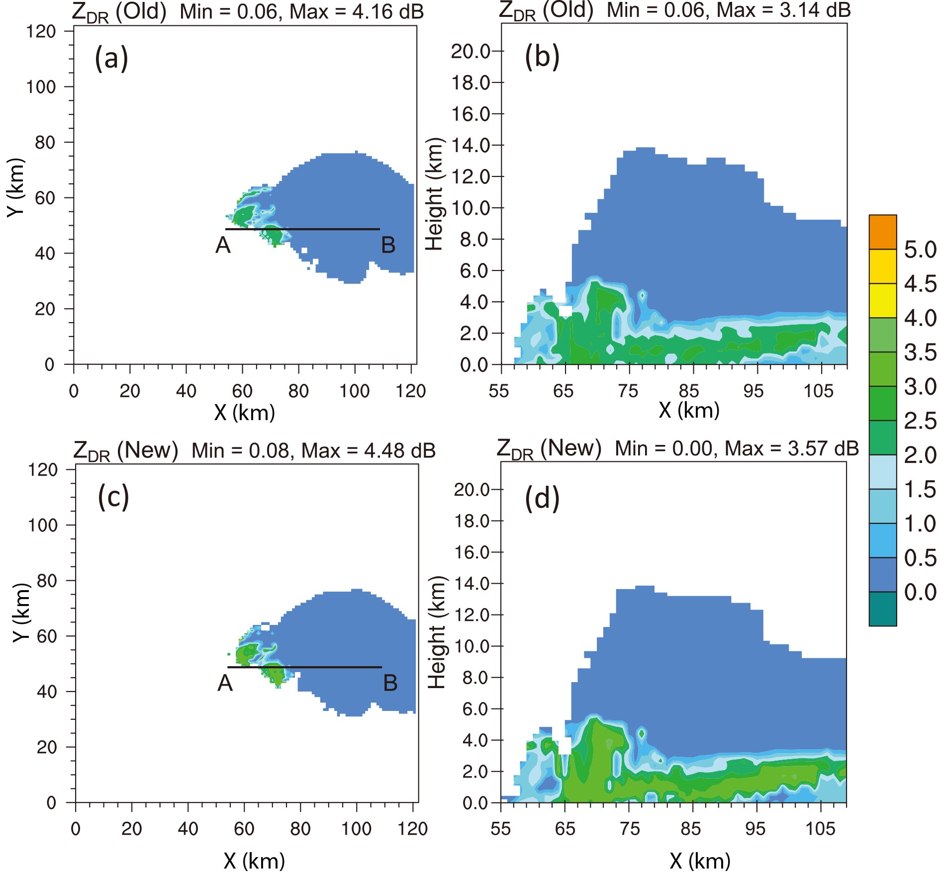Figure5. The same as Fig. 4, but for differential reflectivity (Z_DR).


Figure6. The same as Fig. 4, but for specific differential phase (K_DP).


Figure7. The same as Fig. 4, but for the row co-polar correlation coefficient (ρ_hv).



2 -->

4.2. Real case

To more systematically examine the performance of the new parameterized operators in comparison with the old numerical integration method, a real data case is presented as follows. A volatile weather event occurred across north-central Kansas during the afternoon of May 1, 2018. Multiple supercells spawned a dozen tornadoes including a long track EF-3, though no injuries or fatalities were reported. The event was observed by several operational WSR-88D radars. Here we give an example of the event detected by the KUEX radar in Hastings, Nebraska.
As with the idealized case, the WRF model is used for the simulation of this multiple supercell event. The microphysics used is the same as described earlier. The horizontal grid spacing is 1.5 km with 500 grid points in both the east-west and north-south directions. Vertically, 50 stretched levels up to 20 km above ground level (~50 hPa) are chosen. Radar measured radial velocity data and reflectivity data are assimilated into the WRF model through a variational data assimilation scheme (Gao et al., 2012) with a rapid cycle (every 15 minutes) for two hours from 1900 UTC to 2100 UTC, then a one hour forecast is launched. The reflectivity forecast result at 2200 UTC is compared with the radar reflectivity observations which are interpolated to model grid points for easy comparison. Since the radar best observed this event in the middle levels, radar observations at 5 km above ground level (AGL) are presented for this real data case.
Figure 8 represents the observed and the simulated horizontal reflectivity Z_H at 2200 UTC May 1, 2018, during this event. The Z_H observations show a squall line with several embedded supercells over Nebraska and Kansas, with a maximum reflectivity of 66 dBZ (Fig. 8a). The vertical slice though the model location at x = 155 km shows two supercells extended over 10 km above ground level, though an obvious “cone of silence” exists (Fig. 8b). When examining the simulations, high values of Z_H with comparable values are also present close to the radar observations in both old operators and new operators. Both sets of operators cover a wider area than in the observations. The storm cell line is more reasonable along southwest-northeast direction for the new parameterized operators (Fig. 8e) than that of the old operators in central Nebraska (Fig. 8c). The vertical extension of the two supercells is also well simulated, though a weak spurious cell exists in between two major supercells (Fig. 8d vs 8f).
Figure8. Radar PRD horizontal reflectivity at z = 5 km (a) observed by KUEX radar (through 3D linear interpolation); (c) one-hour model forecast simulated using the numerical integration; (e) one-hour model forecast simulated using the new PRD operators and their corresponding vertical slice through longitude of 98.25^oN near 2200 UTC 1 May 2018 (b, d, f).


In agreement with areas of large Z_H values for the storms, observed Z_DR mostly reaches between 1.0 to 5.0 dB and most of the strong signals are limited to below 15 km AGL, though there are outliers that may push the maximum Z_DR up to 7.9 dB (Figs. 9a, b). For the simulations, the range of values for Z_DR in most areas are close to the observations for both the new and old operators in the area where simulated storms exist. It looks most values related to the model simulation for the new operators are between 1.0 to 4.0 dB (Figs. 9c-9f) which better matches the reflectivity of the storm cores (Fig. 8c-8f). In the vertical direction, the simulated, relatively large values for Z_DR are also limited to below 8 km AGL. In terms of separation of storm cells, the simulated Z_DR cores (Fig. 9f) better match the reflectivity cores (Fig. 8f) using the new operators compared to using the old operators (Fig. 9d vs 8d).
Figure9. The same as Fig. 8, but for differential reflectivity (Z_DR).


For specific differential phase K_DP, the observed values in a range from 2 to 4 ^o km^?1 are closely associated with the main storm areas, which is indicative of strong reflectivity cores (Figs. 10a, 10b vs Figs. 8a, 8b). In the vertical direction, the area of the largest simulated K_DP values is associated with the major supercell in this slice for both the old and new operators, and both agree with the observations in the major storm core (Figs. 10d, f vs Figs. 8d, f). The vertical extension of the high values for K_DP is a little bit deeper than that of Z_DR (Figs. 10d, f vs Figs. 9d, f). This indicates that K_DP may be more useful in terms of identifying strong storms. In this case, the high amounts of null or close to zero values for K_DP are associated with locations where the simulated Z_H is lower than 25 dBZ, corresponding to small amounts of hydrometeor contents simulated by both sets of operators. This is because K_DP has a large relative estimation error in measurements for light precipitation. This feature is consistent with the findings of Thomas et al. (2020).
Figure10. The same as Fig. 8, but for differential reflectivity (K_DP).


Regarding the co-polar correlation coefficient ρ_hv (Figs. 11a, b), the values are very close to 0.96 to 0.97 in the area of the melting layer and above (around 3 km), indicating a composition of mostly mixed liquid and ice hydrometeors. Far from the radar, ρ_hv values increase up to 1, indicating a more homogeneous hydrometeor distribution for small particles. In both simulations (Figs. 11c, e), most of the areas where Z_H is greater than zero dBZ are also associated with a ρ_hv close to 1, corresponding to very homogeneous areas in the observations. Furthermore, the melting layer is visible in the simulation in both sets of the operators (Figs. 11d, f). Mixed phases of hydrometeors in or near melting layers lead to low ρ_hv values, especially for the new operators (Fig. 11f). The simulation results for ρ_hv with the new operators more closely matched the observations than the simulated results obtained using the old operators. (Fig. 11d vs 11f).
Figure11. The same as Fig. 8, but for the co-polar correlation coefficient (ρ_hv).



2 -->

4.3. Comparison of computational efficiency

For the idealized case, it takes 10.55 seconds to run the PRD simulation using the old numerical integration method. In comparison, it takes only 0.098 seconds to complete the simulation with the new parameterized operators on a single node of the University of Oklahoma Supercomputer named Schooner (Table 5). For the real data case, the model domain is bigger. It takes 243.1 seconds for the old operator and 2.287 seconds for the new simplified operators. In general, the new PRD simulation uses less than one percent of the computing time compared to the old one. The PRD operators or simulators can be used in any data assimilation scheme in which PRD can be assimilated into NWP models, such as the WRF model to improve short-term, convective scale, high-resolution NWP forecasts. In such applications, the impact of the new PRD operators with less computational time can be significant because the PRD simulations need to be performed many times until convergence is reached in the DA analysis. The use of the new, more computationally efficient PRD operators may greatly help forecasters or decision-makers quickly deliver their operational products to the public.

Event	Idealized case	Real data case
Old numerical integration operators	10.55	243.1
New parameterized operators	0.098	2.287

Table5. List of computational CPU time (seconds) used for calculating radar variables from WRF model hydrometeor output (domain size is different for idealized and real data cases).

To better and efficiently use PRD, a set of parameterized observation operators are developed to link PRD and NWP model-predicted hydrometeor mixing ratios of rain, snow, hail, and graupel, as well as number concentrations of each species. The model equivalent polarimetric radar variables are calculated based on the T-matrix calculation of wave scattering and the integrations of scattering weighted particle size distribution. These polarimetric radar variables are then fitted to simple functions of water content (or reflectivity factor) and volume-weighted mean diameter of the hydrometeor particle size distribution. The new operators have simple polynomial function forms of hydrometeor mixing ratios and mass/volume-weighted mean diameters, which can be easily implemented and modified. The polynomial form allows for easy calculation of the derivatives for variational analysis.
The parameterized PRD operators are applied to an ideal case and a real case by transferring the WRF model output to equivalent polarimetric radar variables to show the operators’ validity, applicability, and efficiency. A double-moment microphysical parameterization scheme is used during WRF model integration. Considering both case studies, it is generally found that realistic simulations of polarimetric variables can be realized through parameterized and simplified forward operators. The parameterized operators use less than one percent of the computing time of the old PRD simulators to complete the same simulations. The high efficiency in computation and easy implementation/modification make it a good candidate for PRD simulation and assimilation usage.
It is worth to note that the parameterized operators are derived based on the assumptions of constant density for each species of hydrometeor. They are applicable to those NWP models that have microphysical parameterization schemes which contain the same assumptions. Although the parameterized operators are tested on the WRF with double-moment microphysics, they can also be applied to the NWP models with a single moment microphysical parameterization scheme in which the volume-weighted mean diameter can be calculated from the hydrometeor mixing ratio. It is not our intention for the parameterized operators to be used in other model microphysical schemes such as triple-moment parameterization or bin model microphysics.
Acknowledgements. Computing resources were provided by the University of Oklahoma (OU) Supercomputing Center for Education & Research (OSCER).
Open Access This article is distributed under the terms of the Creative Commons Attribution License which permits any use, distribution, and reproduction in any medium, provided the original author(s) and the source are credited. This article is distributed under the terms of the Creative Commons Attribution 4.0 International License (http://creativecommons.org/licenses/by/4.0/), which permits unrestricted use, distribution, and reproduction in any medium, provided you give appropriate credit to the original author(s) and the source, provide a link to the Creative Commons license, and indicate if changes were made.