1.China Institute of Atomic Energy, P. O. Box 275 (10), Beijing 102413, China 2.Key Laboratory of Quark and Lepton Physics (MOE) and Institute of Particle Physics, Central China Normal University, Wuhan 430079, China 3.School of Physics and Center of Excellence in High Energy Physics & Astrophysics, Suranaree University of Technology, Nakhon Ratchasima 30000, Thailand 4.Department of Physics, Naresuan University, Phitsanulok 65000, Thailand Received Date:2019-09-26 Accepted Date:2019-12-10 Available Online:2020-03-01 Abstract:We propose a forward method based on PYTHIA6.4 to study the jet properties in ultra-relativistic pp collisions. In the forward method, the partonic initial states are first generated with PYTHIA6.4 and then hadronized in the Lund string fragmentation model, and finally the hadronic jets are constructed from the created hadrons. Jet properties calculated with the forward method for pp collisions at $\sqrt{s}$=7 TeV are comparable to those calculated with the usual anti-$k_t$ algorithm (backward method) in PYTHIA6.4. The comparison between the backward and forward methods may contribute to the understanding of the partonic origin of jets in the backward method.
HTML
--> --> --> 1.IntroductionIn the early stage of ultra-relativistic heavy ion collisions, the hard parton scatterings generate high transverse momentum partons which traverse the medium and then hadronize into sprays of particles called jets [1]. Jet studies play an important role in understanding the properties of the medium created in ultra-relativistic heavy-ion collisions [2]. The "jet-quenching" together with the "elliptic flow" reveal the essential characteristics of the strongly coupled quark-gluon plasma (sQGP) in the ultra-relativistic heavy ion collisions at the RHIC [3–6] and LHC [7–9] energies. With higher collision energy, higher luminosity, and better detectors for jet measurements, the LHC experiments are able to measure jet properties more precisely. Recently, the ATLAS, CMS, and ALICE collaborations published a series of results of jet properties in pp, p+Pb, and Pb+Pb collisions at the LHC energies [10–17], where new physics has arisen and needs to be studied. The perturbative quantum chromodynamics (pQCD) is able to quantitatively describe the hard parton-parton scattering process and the related initial and final state parton showers. However, one can not apply pQCD directly to describe the properties of particles in jets, as the hadronization of partons is a non-perturbative process. In order to predict the intra-jet properties, phenomenological models have to be employed. Several Monte Carlo (MC) event generators, like PYTHIA6.4 [18], PYTHIA8 [19], HERWIG [20], HERWIG++ [21], and SHERPA [22], are available on the market. The results of MC event generators are sensitive to the model parameters assumed, which must be tuned to fit the experimental data. Consequently, a number of PYTHIA tunes exist, such as the Perugia 2011 tune [23]. In the PYTHIA model, the leading order perturbative QCD (LO-pQCD) is used to generate the $ 2\rightarrow 2 $ hard processes (parton-parton collisions). The parton shower model [24–26] is employed to describe the initial and final state parton radiations. As for the soft (non-perturbative) processes several empirical options are available [27, 28]. Finally, the Lund string hadronization model is used for hadronization of partons [29-31]. In this work, PYTHIA6.4 [18] is employed to investigate the properties of particles in the jets in pp collisions at $ \sqrt{s} $ = 7 TeV using the backward (the usual anti-$ k_t $ algorithm) and the forward methods.
2.Backward method for study of jetsIn the backward method, we first employ PYTHIA6.4 to generate the final hadronic state in pp collisions at $ \sqrt{s} $ = 7 TeV. The jet-finding algorithm, i.e. the anti-$ k_t $ technique [32, 33], is then used to backward reconstruct the jets, as is done in the usual analysis of the experimental data [11]. As it starts from the final hadronic state and proceeds to the reconstructed hadronic jets by searching for their partonic origin, this routine is opposite to the natural time evolution of collisions, as sketched in the left part of Fig. 1. Hence, it is referred to as the backward method. Figure1. (color online) A sketch of the backward and forward methods.
In the anti-$ k_t $ algorithm, the distance $ d_{ij} $ between entities (particle or energetic cluster) i and j is defined as [32]:
and $ k_{ti} $, $ y_i $ and $ \phi_i $ are the transverse momentum, rapidity and azimuthal angle of particle i, respectively. The distance between particle i and beam (B) $ d_{iB} $ is defined as
$ d_{iB} = k^{-2}_{ti}. $
(3)
With the distances $ d_{ij} $ and $ d_{iB} $, a list is compiled containing $ d_{ij} $ and $ d_{iB} $ for all particles in an event. If the smallest entry is $ d_{ij} $, particles i and j are combined (their four-vectors are added) as a jet. If the smallest entry is $ d_{iB} $, particle i is considered as a complete jet and removed from the list. The distances for all entities are recalculated and the procedure repeated until no entities are left. Thus, the distance parameter R in the anti-$ k_t $ algorithm is an essential quantity, within which the particles are reconstructed as a jet. If a hard particle has no hard neighbor within the distance 2R, then it will simply accumulate all soft particles within a circle of radius R, resulting in a perfectly conical jet. If there is another hard particle 2 in the area of $ R < \Delta R_{12} < 2R $, then there will be two jets. The shape of jet $ 1 $ will be conical and jet 2 will be partly conical when $ k_{t1} \gg k_{t2} $; both cones will be clipped when $ k_{t1} \sim k_{t2} $ [32]. The anti-$ k_t $ algorithm is infrared and collinear safe and produces geometrically "conelike" jets, so it is widely used for jet reconstruction in experimental data analysis [10, 15, 16]. The jets are reconstructed from the final hadronic state and are attributed to the initial partonic state. Based on the hadronic final states in pp collisions at $ \sqrt{s} $ = 7 TeV generated by PYTHIA6.4, we use the anti-$ k_t $ algorithm to reconstruct the jets. Following ATLAS [11], the charged particles with transverse momentum $ p_T > $ 300 MeV/c and pseudorapidity $ |\eta|<2.5 $ are counted and the distance parameter R = 0.6 is used. After jet reconstruction, the clusters with $ p_T > $ 4 GeV/c and $ |y|< $ 1.9 are accepted as jets, including those with only one particle in the cluster. The jets are divided into five bins according to their transverse momentum $ p_{{T,\rm jet}} $, namely 4-6, 6-10, 10-15, 15-24 and 24-40 GeV/c. Jets with $ p_T > $ 40 GeV/c and particles that do not belong to any jet are excluded in the calculations. After the reconstruction of a jet using the anti-$ k_t $ algorithm, we calculate the intra-jet particle distributions [11]:
$ N_{\rm ch} $ and $ N_{\rm jet} $ in Eq. (4) are respectively the number of charged particle and jets in a given $ p_{{T,\rm jet}} $ bin. The variable z (known as the fragmentation variable)
$ z = \frac{\vec{p}_{\rm ch}\cdot \vec{p}_{\rm jet}}{|\vec{p}_{\rm jet}|^2} $
(5)
is defined for each charged particle in a jet, and the variable r stands for the radial distance of the charged particle from the axis of the jet,
$ r = \sqrt{(\phi_{\rm ch}-\phi_{\rm jet})^2+(y_{\rm ch}-y_{\rm jet})^2}, $
(6)
and the variable $ p_T^{\rm rel} $ refers to the momentum of the charged particle in a jet, transverse to the jet axis,
where $ \vec{p}_{\rm ch} $ and $ \vec{p}_{\rm jet} $ are the momenta of the charged particle and the jet, respectively.
3.Forward method for study of jetsAlongside the backward method, we propose the forward method for the study of jets. In the forward method, we first employ PYTHIA6.4 [18] with the hadronization switched off temporarily to generate the partonic initial state in pp collisions at $ \sqrt{s} $ = 7 TeV. The partonic initial state is composed of simple strings (without gluons between the two quark ends) and of complex strings (with gluons between the two quark ends). Gluons are first removed from the complex strings, and are then split into quark pairs, such that each quark pair is modeled as a simple string. Hence, the partonic initial state is finally composed only of simple strings. Each simple string in the partonic initial state is hadronized in the Lund string hadronization model (i. e. by the subroutine PYSTRF in PYTHIA 6.4). Hadrons from hadronization of a simple string are first catalogued into two groups (relative to the two quark ends) according to their relative transverse momenta. The hadrons with momenta closer to the momentum of one end of the string are grouped together. For instance, a hadron is grouped as the candidate for the left quark end jet if its relative transverse momentum to the left quark end is less than its relative transverse momentum to the right quark end. The candidate for a quark end jet is the constituent of a jet if its distance relative to the quark end satisfies Eqs. (1) and (2) ($ R = 0.6 $) in the rapidity and azimuthal ($ {y}-\phi $) phase space. Finally, the two quark ends of a simple string are developed into two hadronic jets, with a two-to-two correspondence. The routine for the forward method is as follows: 1) create the partonic initial state by PYTHIA; 2) construct simple strings; 3) each simple string is hadronized individually by the Lund string fragmentation model; 4) the final hadrons from the two quark ends of a simple string are reconstructed into two jets and 5) the final hadronic state is obtained. The process is parallel to the natural time evolution of a collision, as sketched in the right part of Fig. 1, and is referred to as the forward method. 4.ResultsIn order to show the solidity of the forward method, we first employ this method to calculate the final state charged particle transverse momentum and pseudorapidity distributions in pp collisions at $ \sqrt{s} $ = 7 TeV. The results are shown in Fig. 2 (up triangles) together with the CMS experimental data (solid squares) [34]. In the calculations, the K factor, which "multiplies the differential cross section for hard parton-parton processes" in PYTHIA6.4, is tuned to 4, rather than the default value of 1.5. One sees in Fig. 2 that the calculated transverse momentum and pseudorapidity distributions agree well with the CMS data. Hence, the tuned K factor of 4 is applied to all calculations. Figure2. (color online) Transverse momentum (a) and pseudorapidity (b) distributions of the final state charged particles in pp collisions at $ \sqrt s $=7 TeV calculated with the forward method, and compared with the CMS data (taken from Ref. [34]).
The intra-jet charged particle distributions $ F(z, p_{{T,\rm jet}}) $, $ f(p_T^{\rm rel}, p_{{T,\rm jet}}) $ and $ \rho_{\rm ch}(r,p_{{T,\rm jet}}) $ were then calculated using the backward method and compared with the corresponding ATLAS experimental data [11] (analyzed using the anti-$ k_t $ algorithm, i. e. the backward method) in Fig. 3(a)-3(c) for pp collisions at $ \sqrt{s} $ = 7 TeV. We see in this figure that the results of the backward method agree fairly well with the ATLAS data, except $ f(p_T^{\rm rel}, p_{{T,\rm jet}}) $ which is smaller than the ATLAS data at high $ p_T^{\rm rel} $ in the $ p_{T,\rm jet} $ bins 10-15, 15-24 and 24-40. Figure3. (color online) Intra-jet charged particle distributions: (a) $F(z, p_{{T,\rm jet}})$, (b) $f(p_T^{\rm rel}, p_{{T,\rm jet}})$ and (c) $\rho_{\rm ch}(r, p_{{T,\rm jet}})$ in $p_{{T,\rm jet}}$ bins 4-6, 6-10, 10-15, 15-24 and 24-40 GeV/c for pp collisions at $\sqrt{s}$=7 TeV. The solid symbols are the ATLAS data [11] and the open symbols the results of the backward method. The results in the bins 6-10, 10-15, 15-24 and 24-40 GeV/c are multiplied by 10, 102, 103 and 104, respectively. The distance parameter R=0.6 is assumed.
The intra-jet charged particle distributions $ F(z, p_{{T,\rm jet}}) $, $ f(p_T^{\rm rel}, p_{{T,\rm jet}}) $ and $ \rho_{\rm ch}(r,p_{{T,\rm jet}}) $ calculated using the forward and backward methods are compared in Fig. 4(a)-4(c) for pp collisions at $ \sqrt{s} $ = 7 TeV. Fig. 4 shows that the results of the two methods are comparable. One can also see the scaling phenomena in the $ F(z, p_{T,\rm jet}) $ distribution in high $ p_{T,\rm jet} $ bins 10-15, 15-24 and 24-40 for the backward method, and in all $ p_{T,\rm jet} $ bins for the forward method. Figure4. (color online) Intra-jet charged particle distributions: (a) $F(z, p_{{T,\rm jet}})$, (b) $f(p_T^{\rm rel}, p_{{T,\rm jet}})$ and (c) $\rho_{\rm ch}(r, p_{{T,\rm jet}})$ calculated using the forward method compared with the backward method in $p_{{T,\rm jet}}$ bins 4-6, 6-10, 10-15, 15-24 and 24-40 GeV/c for pp collisions at $\sqrt{s}$=7 TeV. The results of the backward method are multiplied by 102.
5.Discussion and conclusionsIn this work, the forward method based on PYTHIA6.4 is proposed to study the properties of intra-jet charged particle distributions $ F(z, p_{{T,\rm jet}}) $, $ f(p_T^{\rm rel}, p_{{T,\rm jet}}) $ and $ \rho_{\rm ch}(r, p_{{T,\rm jet}}) $. The calculated results were compared with the backward method (the usual anti-$ k_t $ algorithm). The ATLAS data (analyzed with the anti-$ k_t $ algorithm) [11] for the intra-jet charged particle distributions $ F(z, p_{{T,\rm jet}}) $, $ f(p_T^{\rm rel}, p_{{T,\rm jet}}) $ and $ \rho_{\rm ch}(r, p_{{T,\rm jet}}) $ in pp collisions at $ \sqrt{s} $ = 7 TeV are well reproduced by the backward method, as shown in Fig. 3. The distributions calculated using the forward method are comparable to the backward method, as shown in Fig. 4(a)-4(c). A comparison of the $ F(z, p_{{T,\rm jet}}) $, $ f(p_T^{\rm rel}, p_{{T,\rm jet}}) $ and $ \rho_{\rm ch}(r, p_{{T,\rm jet}}) $ distributions obtained using the backward and forward methods may shed some light on the correspondence between the final hadronic jets and initial partons in the backward method. The forward method relates the final hadronic jet to its initial partons, which helps to eliminate the effect of combinatorial jets and fake jets. The results of the forward method can also serve as a reference for the backward method in the studies of jets. As mentioned in [1], the key problem in a jet study using the backward method, both experimental and theoretical, is to identify the jets which are generated by the hard scattered partons and to eliminate the effect of combinatorial jets and fake jets. However, this problem does not exist in the forward method, where the final hadronic jets are all constructed directly from the initial partonic strings. Therefore, a comparison between the $ F(z, p_{{T,\rm jet}}) $, $ f(p_T^{\rm rel}, p_{{T,\rm jet}}) $ and $ \rho_{\rm ch}(r, p_{{T,\rm jet}}) $ distributions obtained using the backward and forward methods may help to evaluate and/or to eliminate the effect of combinatorial jets and fake jets in the backward method. The above aspects of the two methods clearly need further studies.


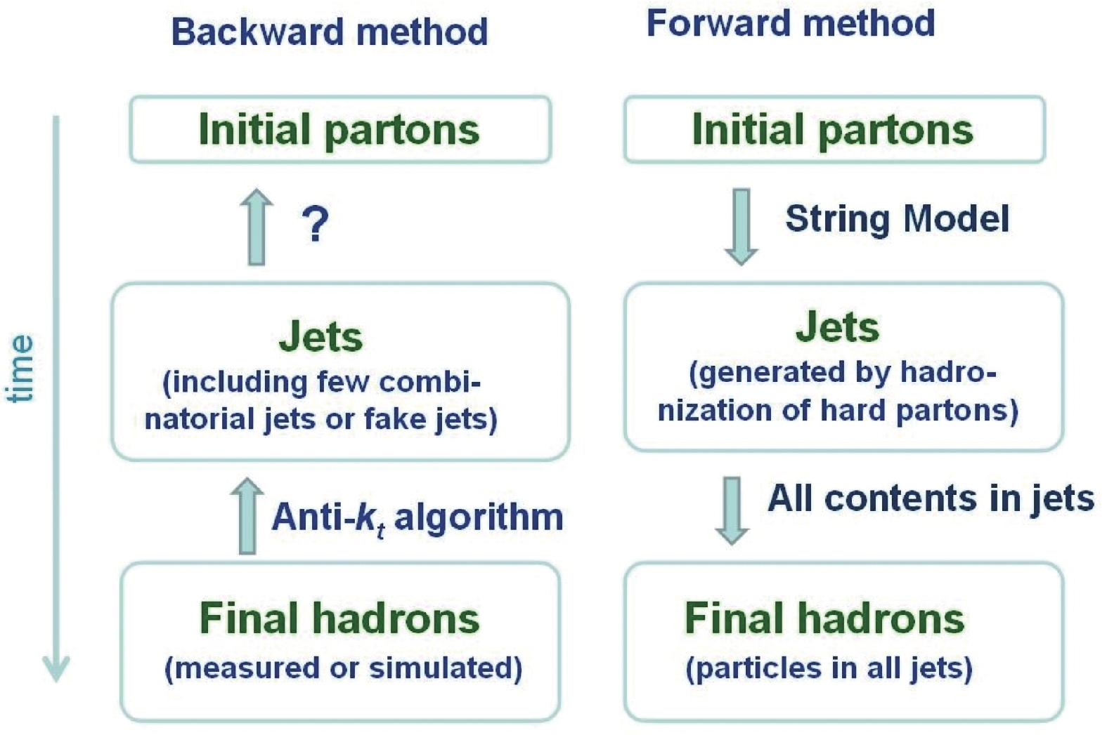 Figure1. (color online) A sketch of the backward and forward methods.


 Figure2. (color online) Transverse momentum (a) and pseudorapidity (b) distributions of the final state charged particles in pp collisions at
  Figure3. (color online) Intra-jet charged particle distributions: (a)
  Figure4. (color online) Intra-jet charged particle distributions: (a)