Daosheng XU^1,,,
Dehui CHEN²,
Kaixin WU¹

Corresponding author: Daosheng XU,dsxu@gd121.cn;

1.Guangzhou Institute of Tropical and Marine Meteorology/Key Laboratory of Regional Numerical Weather Prediction, Guangzhou 510640, China
2.National Meteorological Center, Beijing 100081, China
Manuscript received: 2020-05-06
Manuscript revised: 2020-09-14
Manuscript accepted: 2020-11-10
Abstract:Construction of high-order difference schemes based on Taylor series expansion has long been a hot topic in computational mathematics, while its application in comprehensive weather models is still very rare. Here, the properties of high-order finite difference schemes are studied based on idealized numerical testing, for the purpose of their application in the Global/Regional Assimilation and Prediction System (GRAPES) model. It is found that the pros and cons due to grid staggering choices diminish with higher-order schemes based on linearized analysis of the one-dimensional gravity wave equation. The improvement of higher-order difference schemes is still obvious for the mesh with smooth varied grid distance. The results of discontinuous square wave testing also exhibits the superiority of high-order schemes. For a model grid with severe non-uniformity and non-orthogonality, the advantage of high-order difference schemes is inapparent, as shown by the results of two-dimensional idealized advection tests under a terrain-following coordinate. In addition, the increase in computational expense caused by high-order schemes can be avoided by the precondition technique used in the GRAPES model. In general, a high-order finite difference scheme is a preferable choice for the tropical regional GRAPES model with a quasi-uniform and quasi-orthogonal grid mesh.
Keywords: high-order difference scheme,
dispersion,
uniform,
orthogonal,
computational efficiency
摘要:基于泰勒展开构造高阶精度有限差分方案很早就成为了计算数学界的热门话题，但是它在成熟的数值天气预报模式中仍然很少被应用。为了将高阶精度有限差分方案应用于GRAPES（Global/Regional Assimilation and Prediction System）模式，本文通过理想试验对高阶精度有限差分方案的相关性质进行了分析。一维重力波的线性分析结果表明，在高阶精度差分方案下不同跳点网格方案的影响很小。一维平流试验结果表明：对于网格距离缓慢变化的非均匀网格，高阶差分方案的改进效果仍然十分明显，不连续方波试验的结果也表明了高阶方案的优越性。在地形追随坐标系下的二维质量平流试验结果表明，当模式网格的非均匀性和非正交性变得很明显时，高阶方案的改进效果变得不是很明显。通过在GRAPES模式中采用预条件技术，可以有效地避免高阶方案引起计算量增加的问题。总而言之，对于准均匀和准正交网格的热带区域GRAPES模式来说，发展基于高阶精度有限差分方案的动力框架是一种可行的选择。
关键词:高阶精度差分方案,
频散,
非均匀,
正交性,
计算效率

HTML

--> --> -->

Numerical differentiation is an elementary issue in numerical analysis. Theoretical research in computational mathematics has demonstrated the superior performance of higher-order difference schemes in reducing the truncation error and improving the ability of resolving high-frequency waves (Morinishi et al., 1998; Li, 2005; Lin and Zhan, 2008). Construction of high-order finite difference schemes falls into two categories: (1) The traditional finite scheme, which can be directly expressed by values on the computational grid. However, the number of grid points used for the computation stencil will be increased for higher-order schemes, and the computational efficiency may be reduced. (2) The compact difference scheme, which can limit the number of grid points used in the computation stencil to less than three, regardless of the order of difference schemes. Its weakness lies in the difference scheme cannot be expressed by grid values explicitly. As a result, a set of linear tridiagonal equations need to be solved (Sun et al., 2014).
High-order difference schemes have been widely applied in ocean models. McCalpin (1994) compared 2nd-order and 4th-order pressure gradient algorithms in a sigma coordinate ocean model and found that the higher-order scheme was helpful to improve the accuracy and stability of the model. Chu and Fan (1997, 2000) further implemented a 6th-order difference scheme in a sigma ocean model to reduce the truncation error in calculating the horizontal pressure gradient term. A control-volume ocean model with a 4th- and 5th-order finite difference scheme was presented by Sanderson and Brassington (2002).
The accuracy of discretization for dynamic equations in numerical weather prediction (NWP) is an important issue for its performance, so how to design accurate high-order schemes for NWP models has long been a research focus (Cullen and Davies, 1991; Lin and Rood, 1996; Yang et al., 2015). Sch?r et al. (2002) demonstrated the beneficial impact on reducing small-scale noise by higher-order difference schemes with an idealized advection test. Feng and Li (2007) developed a high-order upwind-biased difference scheme, and tested its computational performance with the one-dimensional advection equation and inviscid Burgers’ equation. A high-order positive-definite conservative multi-moment center constrained finite volume transport model was presented by Shu et al. (2020) to improve the moist transport in NWP models.
In recent years, construction of dynamic cores with high accuracy has become one of the main international trends in developing new-generation NWP models. The truncation error of the GFDL finite volume cubed-sphere dynamical core (FV3, Lin, 2004 2008) reached 3rd order. Li et al. (2015) built a 3rd- and 4th-order multi-moment constrained finite-volume method and tested it with a global shallow-water model on the Yin–Yang grid. At present, a central difference scheme with 2nd-order accuracy is still applied for the horizontal discretization of the Global-Regional Assimilation and Prediction System (GRAPES) model, which severely limits its computational performance. It will be meaningful to introduce a higher-order difference scheme for the horizontal discretization in the GRAPES model.
Considering the difficulty of coupling the compact difference scheme with a semi-implicit and semi-Lagrange time discretization scheme in the GRAPES model, we adopted the traditional finite difference scheme to construct a higher-order dynamic core. As the application of high-order difference schemes in operational NWP models is still very rare, their properties need to be further investigated before being implemented in the GRAPES model, which is the main purpose of this paper. The equations of high-order schemes based on Taylor series is displayed in section 2. Dispersion properties of high-order schemes are presented in section 3, and the performance under non-uniform and non-orthogonal grid conditions is presented in sections 4 and 5. Section 6 discusses the impact of high-order finite difference schemes on computational efficiency when implemented in the GRAPES model. Finally, a summary and discussion are provided in section 7.

The equations for finite difference schemes with 2nd-, 4th- and 6th-order accuracy are displayed in Table 1 (for details of derivation, see Appendix A). The number of grid points used in the computational stencil increases from three to seven with the accuracy raised from 2nd to 6th order, so it is an important issue to deal with the computational efficiency problem for application of high-order finite difference schemes.

	Unstaggered grids	Staggered grids
2nd order	$ \dfrac{{f}_{i+1}-{f}_{i-1}}{2\Delta x} $	$ \dfrac{{f}_{i+0.5}-{f}_{i-0.5}}{\Delta x} $
4th order	$ \dfrac{{f}_{i-2}-8{f}_{i-1}+8{f}_{i+1}-{f}_{i+2}}{12\Delta x} $	$ \dfrac{{f}_{i-1.5}-27{f}_{i-0.5}+27{f}_{i+0.5}-{f}_{i+1.5}}{24\Delta x} $
6th order	$ \dfrac{-{f}_{i-3}+9{f}_{i-2}-45{f}_{i-1}+45{f}_{i+1}-9{f}_{i+2}+{f}_{i+3}}{60\Delta x} $	$ \dfrac{-9{f}_{i-2.5}+125{f}_{i-1.5}-2250{f}_{i-0.5}+2250{f}_{i+0.5}-125{f}_{i+1.5}+9{f}_{i+2.5}}{1920\Delta x} $
Notes: $ f $ represents an arbitrary function, and $ \Delta x $ represents grid length in discretization.

Table1. Difference schemes with 2nd-, 4th- and 6th-order accuracy for the first derivative under unstaggered and staggered grids.


The Fourier analysis of error for difference schemes for first- and second-derivative approximation under an unstaggered grid is shown in Fig. 1 (for the detailed process of derivation, see Appendix B). The improvement of the higher-order schemes in resolving short waves is significant, especially from 2nd- to 4th-order accuracy.
Figure1. Fourier analysis of error for the first derivative approximation with different schemes under an unstaggered grid.

Dispersion of ageostrophic atmospheric energy with gravity waves is the physical mechanism of geostrophic adjustment. The dispersion property is an important criterion to evaluate the performance of the model dynamic core. In this paper, a one-dimensional gravity wave equation (Arakawa and Lamb, 1977) is adopted to investigate the dispersion properties of high-order difference schemes:
where u and v are the horizontal components of wind in the x and y directions, h is the depth of fluid, $ f $ is a constant Coriolis parameter, $ g $ is gravity, and H is the mean of h. If the solution is assumed proportional to $ {\rm{exp}}\left[i(kx-\nu t)\right] $ (k is the wave number), then the angular frequency $ \nu $ for the inertia gravity is given by
where L is the wavelength in the x direction.
The effect of space discretization error can now be examined. The following frequencies are obtained for Arakawa-A and Arakawa-C grids (the radius of deformation $ \lambda $ defined by $ {\sqrt{gH}}/{f} $, and $ d $ is the grid size):
A grid + 2nd order:
A grid + 4th order:
A grid + 6th order:
C grid + 2nd order:
C grid + 4th order:
C grid + 6th order:
As shown by Fig. 2, the frequencies get closer to the true solution when higher-order difference schemes are applied, both in the A grid and C grid for $ \lambda /d=2 $. The dispersion error of the 2nd-order scheme in the A grid is significant for low wavenumber area (wavelength longer than four grid-interval, as indicated by the blue rectangle in Fig. 2), while the 4th- and 6th-order schemes in the A grid are as good as the C grid. For the grid scale wave ($ L/d<4 $), the dispersion error of the C grid is much better than that of the A grid. Considering high-frequency waves cannot be resolved well by the model grid, they need to be filtered out to avoid nonlinear instability. Therefore, poor dispersion properties of the A grid at the grid scale are not problematic as long as such waves can be selectively removed. This conclusion is consistent with the research of Chen et al. (2018).
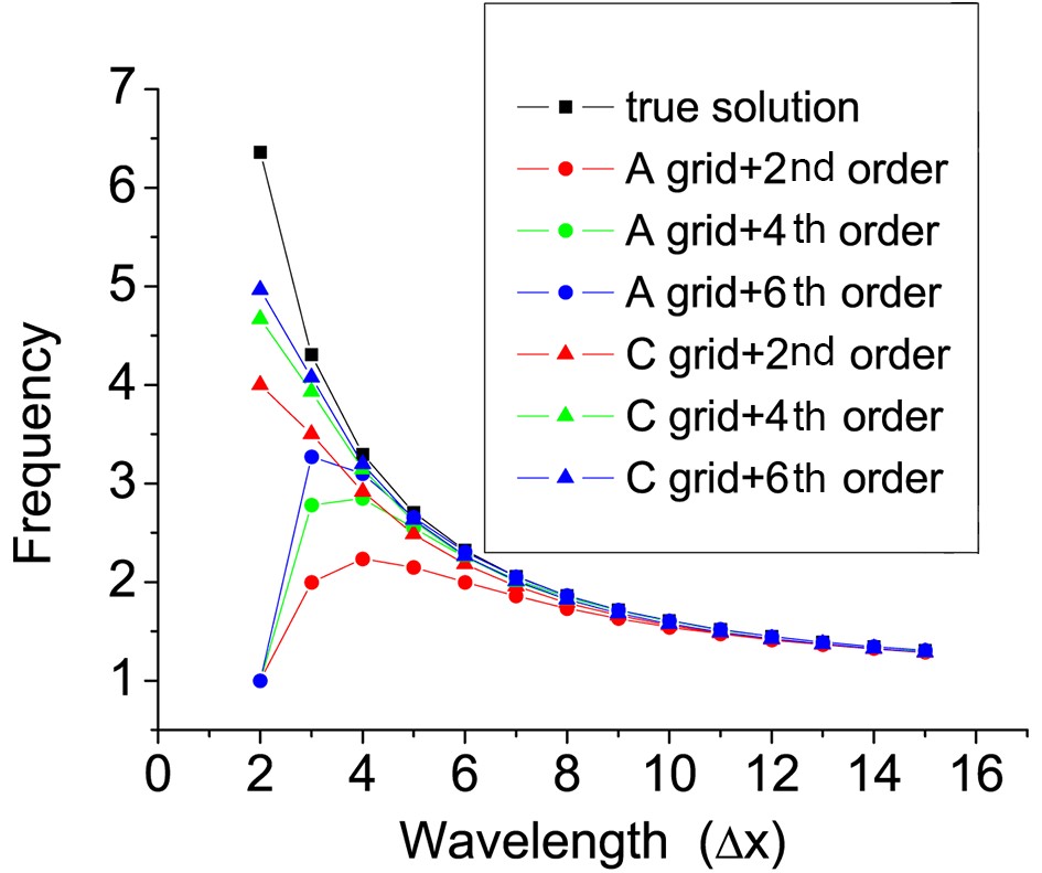Figure2. The dependency of (nondimensional) frequency $ \upsilon /f $ on the wavelength for the case $ \lambda /d=2 $.

The equations displayed in Table 1 are derived under the hypothesis of a uniform grid, but this hypothesis is not always strictly satisfied in NWP models. For example, the grid interval of the latitude–longitude grid applied in the GRAPES model will get smaller at higher latitude, and the distribution of vertical model levels are also designed to be non-uniform (Xue and Chen, 2008). The accuracy of higher-order difference schemes will be degenerated under a non-uniform grid (Xu and Chen, 2020).
The performance of higher-order schemes under a non-uniform grid is investigated with the following one-dimensional advection equation based on an unstaggered grid:
Here, $ u $ is an arbitrary scalar, and $ \alpha $ is defined as a constant.

2

-->

4.1. Test with a smooth wave solution

When the initial value is set as $ u\left(x,0\right)= A{\rm{sech}}\left(kx\right) $, the true solution of Eq. (11) can be written as $ u\left(x,t\right)= A{\rm{sech}} $$ \left[k(x+\alpha t)\right] $, where A is a parameter defined as a constant, and $ {\rm{sech}} $ means the hyperbolic secant function (Li, 2012). This equation describes the translational motion of a solitary wave being advected to the left, and the choice of the inverse hyperbolic secant function was based on the consideration of testing the high-order scheme with a modal, smooth solution. The parameters are set as follows: A = 1.0, k = 0.5, $ \alpha $ = 2.0, $ x\in \left[-40,20\right] $, and an Euler scheme is adopted for time integration with the timestep $ \Delta t $ =1×10^?3. Three sets of grid configuration are designed as follows to assess the performance of high-order schemes under the non-uniform grid:
Uniform grid:
Nonuniform grid ? 1:
Nonuniform ? grid ? 2:
The grid spacing is gradually reduced in Non-uniform-grid-1 from left to right, while the opposite is the case in Non-uniform-grid-2. As shown in Fig. 3, the dissipation and phase errors of the nonuniform and uniform grid are very close to each other, which implies that the dissipation and dispersion properties of higher-order difference schemes will not be degenerated by the weak uniformity of grids. The improvement from the 2nd-order scheme to the 4th-order scheme is most obvious, while the difference between the 4th-order scheme and the 6th-order scheme is very small. This is consistent with the result of Fourier analysis in section 2. The results of the tests for nonuniform-grid-1 and nonuniform-grid-2 are very similar to each other, which also supports the conclusion that weak non-uniformity will not influence the performance of high-order difference schemes.
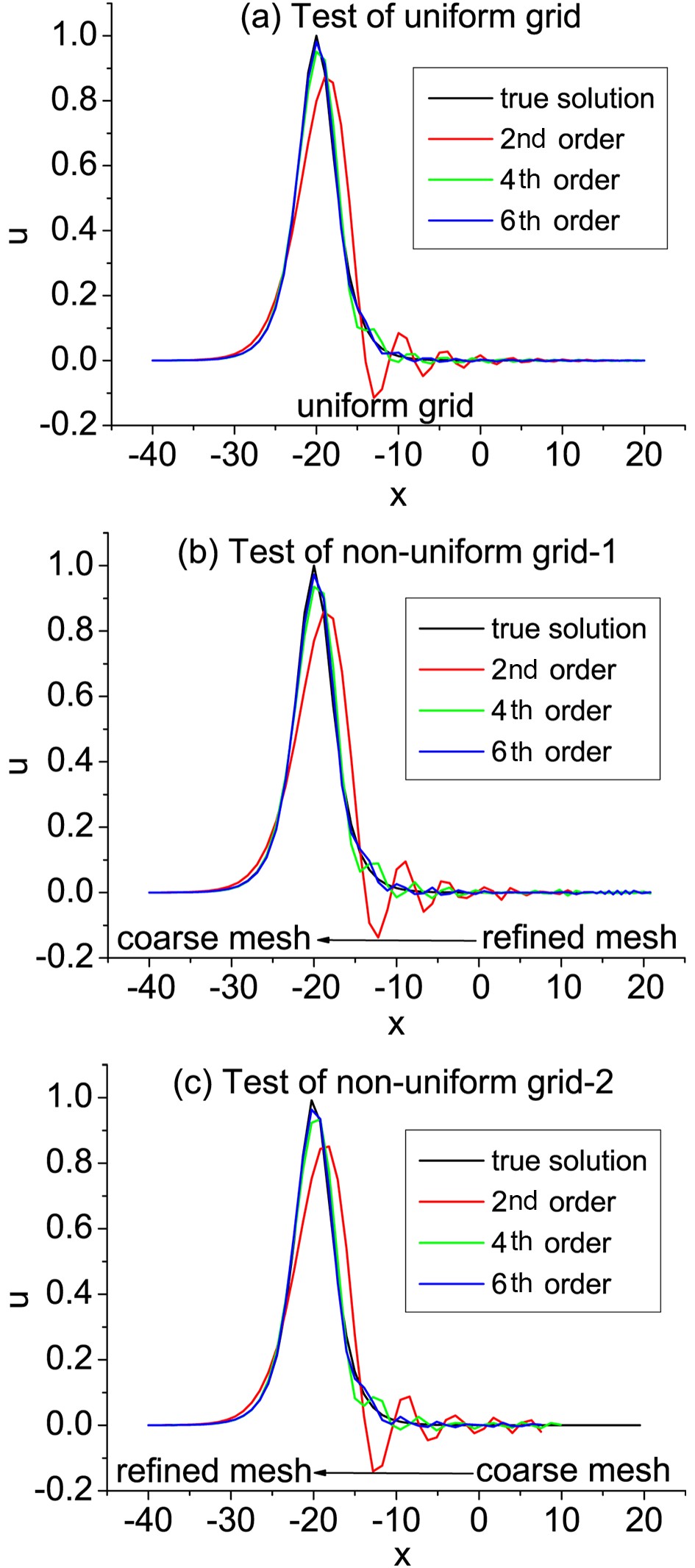Figure3. Numerical test of the one-dimensional advection equation at t = 10 s in (a) a uniform grid, (b) non-uniform grid-1, and (c) non-uniform grid-2.


In general, the higher-order difference scheme are still effective for the non-uniform grid if the variation of grid distance is smooth, so they are applicable for the longitude–latitude grid of the GRAPES model and the non-uniform vertical difference process.

2 -->

4.2. Test with a square wave solution

To study the performance of high-order difference schemes under more discontinuous conditions, a square wave test was further performed. In the square wave test, the initial value of the one-dimensional advection equation [Eq. (11)] was set as
The parameters were set the same as in section 4.1, and the advection test was performed under a uniform grid. Figure 4 shows the simulated square signals at t = 1 s. The overshoot and undershoot noise were alleviated by the higher-order (4th- and 6th-order) schemes. This implies that the advantages of high-order schemes can be extended to the non-modal solutions, although the theoretical analysis is difficult.
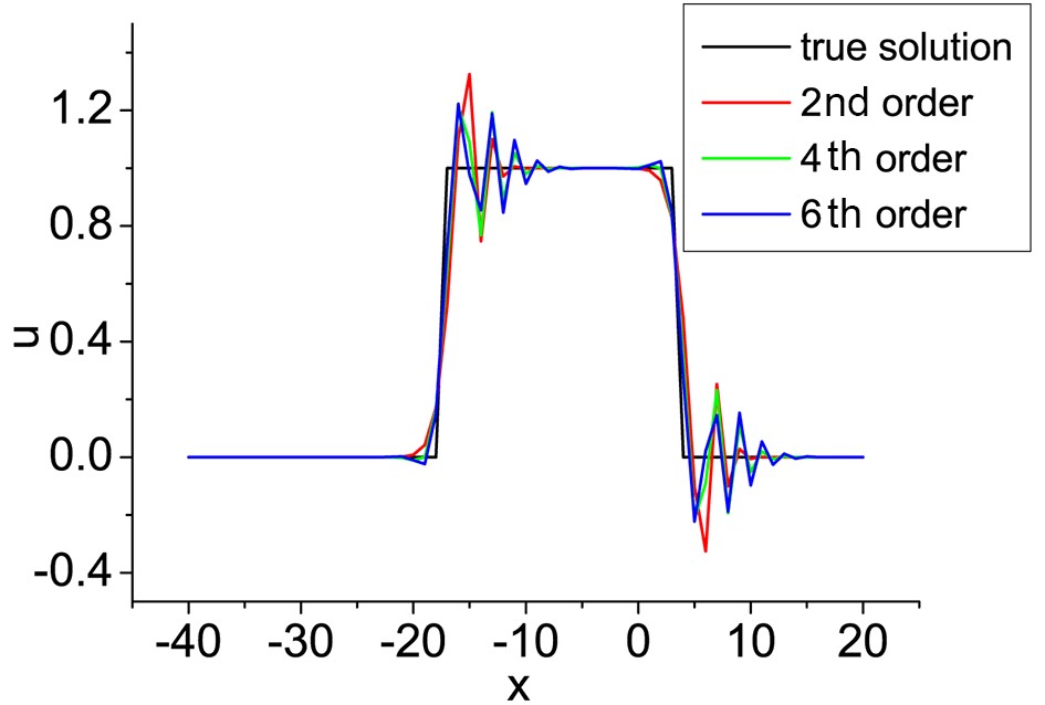Figure4. The result of the square test at t = 1 s.

The performance of high-order difference schemes under a vertical non-orthogonal grid with the terrain is further investigated with an idealized advection test (Sch?r et al., 2002) in this section. It provides a somewhat severe way of testing the effect of non-uniformity on a numerical scheme, as the non-orthogonality and non-uniformity of a terrain-following coordinate is much more severe than it will be on any horizontal grid.
The two-dimensional advection equation under a terrain-following vertical coordinate can be written as (Li et al., 2012)
where $ \rho $ is the density of air, $ z $ is the geometric height, $ \hat{z} $ is the transformed height of $ z $ under the terrain-following coordinate, $ \varphi $ is the stream function defined by $ \varphi \left(z\right)= -{\int }_{0}^{z} $$ u\left(z\right){\rm{d}}z $, $ u $ denotes the wind speed along the x direction, and $ {J}_{b}^{-1}=\partial z/\partial \hat{z} $ is the parameter for transformation. Variables $ \rho $ and $ \varphi $ in Eq. (12) are arranged in a staggered grid, and a leap frog scheme is adopted for time integration. The terrain-following vertical coordinate developed by Gal-Chen and Somerville (1975) is adopted in this paper, defined as $ \hat{z}={Z}_{\rm{T}}\dfrac{z-{Z}_{\rm{s}}\left(x\right)}{{Z}_{\rm{T}}{-Z}_{\rm{s}}\left(x\right)} $, where $ {Z}_{\rm{T}} $ is the model top and $ {Z}_{\rm{s}}\left(x\right) $ is the topographic height. The topography $ {Z}_{\rm{s}}\left(x\right) $ is specified as the product of a large-scale mountain $ {Z}_{\rm{s}}^{*}\left(x\right) $ of half width r₀, and a small-scale wavelike perturbation of wavelength $ {L}_{0} $; that is,
where
and where $ {z}_{0} $ denotes the maximum height of the obstacle. In the following test we use $ {z}_{0} $ = 3 km, $ {r}_{0} $ = 25 km, and $ {L}_{0} $ = 8 km. As shown in Fig. 5, the influence of the terrain on vertical levels is significant in the low level, and gradually disappears near the model top, so the computational mesh is non-orthogonal above the terrain.
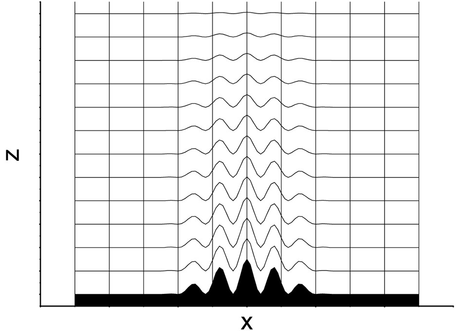Figure5. Schematic diagram of the non-orthogonal grid mesh for the two-dimensional advection test (black shaded area denotes the topographic obstacle).


In the idealized advection test, the topographic obstacle is submerged within a stagnant air mass, but aloft there is a uniform and purely horizontal flow directed from left to right (shown in Fig. 6). The anomaly is assigned the shape
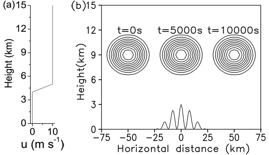Figure6. Vertical cross section for the idealized two-dimension advection test: (a) vertical distribution of velocity u; (b) analytical solution of the density as advected for three instances.


with $r=\sqrt{{\left[(x-{x}_{0})/{R}_{x}\right]}^{2}+{\left[(z-{z}_{0})/{R}_{z}\right]}^{2}}$, and initialized at $ {t}_{1} $ = 0 at location ($ {x}_{0},{z}_{0} $) = (?50 km, 9 km) with amplitude $ {\rho }_{0} $ = 1 and half widths $ {R}_{x} $ = 25 km, $ {R}_{z} $ = 3 km. At time $ {t}_{2} $ = 2500 s, the anomaly is centered right over the mountain and the integrations are terminated at $ {t}_{3} $ = 5000 s. The sheared wind profile is specified as
where $ {u}_{0} $ = 10 m s^?1, $ {z}_{1} $ = 4 km, $ {z}_{2} $ = 5 km. The time step is 25 s, with grid increments of $ \Delta x $ = 1 km and $ \Delta z $ = 500 m. The total number of vertical levels is 51 and the top height is 25 km.
The error fields for the 2nd-, 4th-, and 6th-order difference schemes are displayed in Fig. 7. As the anomaly is located over the obstacle (at t = 5000 s), the reduction of spurious small-scale distortion errors caused by higher-order schemes is obvious at the right-upper side of the obstacle (see Figs. 7a, c and e), although the orthogonality of the grid is partly influenced by the terrain. The improvement is much more apparent when the computational accuracy is increased from 2nd to 4th order. When the non-orthogonality gets much more severe, the forecast error (see the error above the terrain at t = 10000 s in Figs. 7b, d and f) is almost the same for different schemes.
Figure7. Numerical error of difference schemes for the two-dimensional advection equation: (a, b) 2nd-order scheme; (c, d) 4th-order scheme; (e, f) 6th-order scheme; (a, c, e) t = 5000 s; (b, d, f) t = 10000 s.


In general, the performance of high-order difference schemes highly depends upon the orthogonality of the model grid, and the advantage of high-order difference schemes can still be retained when the grid is nearly orthogonal.

The numbers of grids used in the calculation stencil will be increased if higher-order finite difference schemes are applied, so it is an important issue to consider the influence of high-order difference schemes on the computational efficiency for large-scale computation in operational NWP models. In this section, the stencils for the 2nd- and 4th-order difference scheme are compared based on the forecast equations of the GRAPES model, and the influence on the actual computational efficiency is discussed.
The dynamic equation of the GRAPES model under a spherical coordinate system can be written as (Chen and Shen, 2006)
where ${u_{n + 1}}$,${v_{n + 1}}$,${\hat w_{n + 1}}$,$\theta _{n + 1}^{'}$, and $\Pi _{n + 1}^{'}$ denote the forecasted three-dimensional wind components, perturbed potential temperature and perturbed non-dimensional pressure at the n + 1 timestep, respectively. The symbols λ and φ are the longitude and latitude, respectively, and $\hat z$ is the height in the terrain-following vertical coordinate. ${\xi _{x1}}$,${\xi _{x2}}$ and ${\xi _{x3}}$$(x = u,v, $$ \hat w,{\theta ^{'}},{\Pi ^{'}})$ are grid metric coefficients, while ${\xi _{x0}}(x = u,v,\hat w, $$ {\theta ^{'}},{\Pi ^{'}})$ is changed every time-step. ${D_3}$ is the three-dimensional divergence term, and ${A_\Pi }$ is the time discretization term. Equations (14)–(18) can be transformed to a Helmholtz equation of $\Pi $(which is the stencil of the GRAPES model) under the 2nd-order difference scheme:
where ${B_1}$–${B_{19}}$ are the coefficients of 19 grids of the stencil. If the 4th-order scheme is used for horizontal discretization, the Helmholtz equation contains 47 grids (the detail derivation process is omitted):
The generalized conjugate residual (GCR) method is used to solve the Helmholtz equation in the GRAPES model. To accelerate the speed of convergence, a preconditioned algorithm is applied to simplify the coefficient matrix. According to the fact that the coefficients at points ($i,j,k$), ($i,j,k - 1$) and ($i,j,k + 1$) are an order of magnitude larger than other points, the preconditioned matrix only retains these three points’ coefficients and then it becomes a segmented tridiagonal matrix (e.g., Xue and Chen, 2008, pp. 132–136). The magnitude of coefficients at 47 points under the 4th-order scheme are displayed in Table 2, and we also find that the coefficients at points ($i,j,k$), ($i,j,k - 1$) and ($i,j,k + 1$) are an order of magnitude larger than other points. As a result, the preconditioned matrix is the same as the 2nd-order scheme, which implies that the time used to solving the Helmholtz equation will not be increased, and so a higher-order difference scheme is a feasible choice for the GRAPES model.

Coefficient	Magnitude	Coefficient	Magnitude
B1	100	B16–B19	10?4
B2–B4	10?2	B20–B23	10?3
B5–B9	10?8	B24–B35	10?8
B10, B15	10?1	B36–B43	10?5
B11–B14	10?5	B44–B47	10?5

Table2. Magnitude of coefficients in Eq. (27).

To go beyond the well-worn traditional linear shallow-water uniform-grid analyses into somewhat more realistic testing frameworks that consider situations of use in comprehensive weather and climate models, the properties of higher-order difference schemes were investigated for application in the GRAPES model in this paper. The one-dimensional gravity wave equation was used to study the dispersion properties of high-order schemes. Obvious reduction in the dispersion error was found in the higher-order schemes with an Arakawa-A grid for those well-resolved waves, especially from 2nd- to 4th-order accuracy, while the improvement for the Arakawa-C grid was not so apparent. Based on the discovery that the dispersion errors are almost equivalent for the A- and C-grid under 4th- and 6th-order schemes, the possibility of an unstaggered GRAPES dynamical core, which is more convenient to couple with physical processes (Purser and Leslie, 1988), will be further investigated in the future. The preferable properties of high-order difference schemes are still obvious under a non-uniform grid when the variation of grid distance is smooth. The square wave test also indicated the superiority of high-order schemes. For a grid mesh with severe non-orthogonality and non-uniformity, the advantages of high-order schemes are not so obvious, as demonstrated by the results of idealized two-dimensional advection tests. The number of grid points used in the computational stencil will be increased for higher-order schemes, but it will not reduce the computational efficiency of the GRAPES model when the precondition technology being applied to reduce the magnitude of condition number and improving the convergence rate of the GCR.
In general, a high-order finite difference scheme is a feasible choice for a high-resolution, longitude–latitude grid model with a nearly uniform and orthogonal regional domain—for example, the Tropical Regional Area Model System (TRAMS; Xu et al., 2015) developed by the Guangzhou Institute of Tropical and Marine Meteorology, based on the regional version of GRAPES.
Although the result of the two-dimensional advection test under a terrain-following coordinate is in a similar spirit to the analysis of Reinecke and Durran (2009), it can still be misleading since reflections in the one-way advection equation are nearly always into grid-scale wavelengths that are easily diffused for a relatively long-term simulation (Harris and Durran, 2010). Extending a similar test to a more dynamically active case supporting upstream physical wave propagation (Vichnevetsky, 1987) will be more meaningful. A complete study of the performance by implementing high-order schemes in TRAMS will be the next stage in our work. A general finite high-order difference scheme applicable in a non-uniform grid will also be investigated in the future.
Acknowledgements. This work was supported by the National Natural Science Foundation of China (Grant No. U1811464) . We thank the two anonymous reviewers and the editors for their comments, which greatly improved this paper.
APPENDIX ADerivation of High-Order Difference Schemes based on the Taylor Series Expansion Method
The general finite difference equations with arbitrary order accuracy are deduced first, followed by the specific forms of the 2nd-, 4th- and 6th-order schemes.
1.????Equations of traditional finite difference schemes with?????? arbitrary order accuracy
The method to deduce high-order difference schemes at one point can be summarized as follows: the number of grid points needed for the required accuracy is determined first; then the expression of derivatives including indefinite coefficients are deduced; and finally these indefinite coefficients will be obtained by solving the set of simultaneous equations based on Taylor series expansion.
The following 2n + 1 grid will be used to contract 2n-order accuracy schemes for the first derivative:
The expansion of derivations can be written as (with coefficients undetermined):
The function $ f $ is then expanded at point $ i $ with a $ 2n $-order Taylor series:
$ 2n+1 $ equations are obtained by substituting Eq. (A2) into Eq. (A1), and the corresponding $ 2n+1 $ indefinite coefficients can be solved for the detailed expression of the difference scheme. Let $ {\left({{\partial }^{0}f}/{\partial {x}^{0}}\right)}_{i}={f}_{i} $ (zero-order derivations of $ f $ is itself), and (A2) can be expanded as follows (only the first three terms are displayed):
2.????Second-order difference scheme
Let $ n=1 $ in Eqs. (A1)–(A2), and the expressions of the second-order scheme can be obtained. The first derivative equation in Eq. (A1) can be rewritten as follows:
Substituting Eq. (A3) and Eq. (A6) into Eq. (A9), and omitting the remainder terms, we can obtain:
The following coefficients can be derived by equaling the corresponding terms in Eq. (A10):
The 2nd-order finite difference scheme for the first derivative can now be expressed as:
3.????Fourth-order difference scheme
Let n = 2 in Eqs. (A1)–(A2), and the expression of the 4th-order scheme can be obtained. The expansion of Eq. (A1) is
Substituting Eqs. (A3)–(A4) and Eqs. (A6)–(A7) into Eq. (A13),
where
The 4th-order finite difference scheme for the first derivative can now be expressed as:
4.????Sixth-order difference scheme
Let n = 3 in Eqs. (A1)–(A2), and the expression of the 6th-order scheme can be obtained. The expansion of Eq. (A1) is
Substituting Eqs. (A3)–(A5) and Eqs. (A6)–(A8) into Eq. (A17), and omitting the remainder terms, we can obtain:
where
The 6th-order finite difference scheme for the first derivative can now be expressed as:
For the staggered grid, the following 2nd-, 4th- and 6th-order finite difference schemes can be obtained with a similar method:

For an arbitrary periodic function $ f\left(x\right) $ with its wavenumber defined as $ \alpha $, the Fourier transform (represented by F{}) of $ f\left(x\right) $ and $ {\partial f\left(x\right)}/{\partial x} $ is
According to the properties of Fourier transition, we can get
where $ \Delta x $ is the grid distance. The differencing of the 2nd-order approximation for the first derivative under an unstaggered grid can be expressed as:
and its Fourier analysis error can be obtained by performing the Fourier transform on both sides of Eq. (B5):
Hence,
With the wavelength defined as $ L={2\pi }/{\alpha } $, Eq. (B7) can be rewritten as
where $ \tilde L $ is the modified wavelength for the difference scheme with 2nd-order accuracy.
The following Fourier analysis error of the 4th- and 6th-order approximations can be derived with a similar method:
4th-order scheme:
6th-order scheme: