 ,, 刘方东, 邢光南, 王吴彬, 赵团结, 管荣展, 盖钧镒,*南京农业大学大豆研究所 / 农业部大豆生物学与遗传育种重点实验室 / 国家大豆改良中心 / 作物遗传与种质创新国家重点实验室, 江苏南京 210095
Characterization and Analytical Programs of the Restricted Two-stage Multi- locus Genome-wide Association Analysis
HE Jian-Bo,, LIU Fang-Dong, XING Guang-Nan, WANG Wu-Bin, ZHAO Tuan-Jie, GUAN Rong-Zhan, GAI Jun-Yi,*Soybean Research Institute / National Center for Soybean Improvement, Ministry of Agriculture / Key Laboratory of Biology and Genetic Improvement of Soybean (General), Ministry of Agriculture / State Key Laboratory for Crop Genetics and Germplasm Enhancement, Nanjing Agricultural University, Nanjing 210095, Jiangsu, China通讯作者:
第一联系人:
收稿日期:2018-03-19接受日期:2018-06-12网络出版日期:2018-06-29
| 基金资助: |
Received:2018-03-19Accepted:2018-06-12Online:2018-06-29
| Fund supported: |

摘要
关键词:
Abstract
Keywords:
PDF (1557KB)元数据多维度评价相关文章导出EndNote|Ris|Bibtex收藏本文
本文引用格式
贺建波, 刘方东, 邢光南, 王吴彬, 赵团结, 管荣展, 盖钧镒. 限制性两阶段多位点全基因组关联分析方法的特点与计算程序[J]. 作物学报, 2018, 44(9): 1274-1289. doi:10.3724/SP.J.1006.2018.01274
HE Jian-Bo, LIU Fang-Dong, XING Guang-Nan, WANG Wu-Bin, ZHAO Tuan-Jie, GUAN Rong-Zhan, GAI Jun-Yi.
基于全基因组高密度单核苷酸多态性(single- nucleotide polymorphism, SNP)分子标记的全基因组关联分析(genome-wide association study, GWAS)已经成为数量性状遗传基础解析的重要方法。GWAS充分利用了自然群体大量的历史重组事件, 具有较高检测精度, 已广泛应用于动植物复杂性状基因的发掘, 其理论方法与应用也是近十几年来数量性状研究的热点[1]。然而, 自然群体通常具有的群体未知结构会对GWAS产生干扰, 从而导致检测结果较高的假阳性。目前, 考虑群体结构矫正的GWAS统计方法主要包括结构关联法(structured association, SA)[2]、主成分分析法(principal components analysis, PCA)[3]和混合模型方法(linear mixed model, LMM)[4,5,6,7]。结构关联法首先利用基于模型的聚类程序如STRUCTURE[8]、ADMIXTURE[9]等推断获得群体结构, 然后将群体结构作为模型协变量进行关联测验。主成分分析法是将基于分子标记的遗传关系矩阵特征向量作为模型协变量进行关联测验。混合模型方法是在结构关联法和主成分分析法的基础上再将遗传背景效应作为随机效应加入分析模型, 并将基于分子标记的亲属关系矩阵作为该随机效应的协方差结构, 从而同时控制群体结构和家系结构, 该方法也是目前植物GWAS的常用方法[10,11,12,13]。
植物中GWAS通常将种质资源群体作为试验群体, 此类群体存在广泛的遗传变异, 且普遍存在复等位基因。植物育种实质上是一个优异等位基因的聚合过程, 因此复等位基因的检测及其效应估计对植物育种极其重要, 优异等位基因的发掘不仅能为分子标记辅助选择提供依据, 更是设计育种的前提条件[14]。然而以往GWAS方法使用的SNP分子标记在一个标记位点上仅有2个等位变异, 自然无法估计资源群体中大量存在的复等位基因效应, 从而限制了其在植物育种中的应用。尽管GWAS在数量性状遗传研究中发挥了重要作用, 但由于以往GWAS方法注重于个别主要QTL/基因的检测与发掘, 通常使用较为严格的显著水平进行多重测验矫正, 如Bonferroni矫正方法使用0.05/m作为全基因组显著水平, 其中m为标记数目。这种严格的显著水平将可能导致较高的假阴性, 检测的关联位点往往仅能解释表型变异的微小部分, 不能全面解析全基因组遗传位点。例如水稻中41个性状的GWAS结果显示平均每个性状仅能检测到5个位点, 解释大约22%的表型变异[15,16]。因此, 为提供种质资源群体遗传构成信息, 有必要相对全面地检测全基因组QTL。另外, 上述常用GWAS方法均基于单位点模型, 当控制数量性状的位点有多个时, 每个位点的效应估计可能会受到相邻位点的影响[17], 最明显的表现就是导致位点表型变异解释率估计的膨胀, 同时对小效应位点的检测功效也可能会偏低。然而由于全基因组关联分析通常涉及海量的分子标记, 直接将单位点遗传模型扩展至多位点遗传模型的最大难题是模型中变量个数远远超过观测值数目, 无法直接求解, 从而限制了多位点模型在GWAS中的应用。针对上述GWAS在植物应用中的局限性, He等[18]通过合并多个相邻且紧密连锁的SNP标记组成具有复等位变异的SNPLDB标记, 并基于多位点复等位基因模型进行全基因组QTL检测, 提出了限制性两阶段多位点全基因组关联分析方法(RTM-GWAS)。该方法解决了GWAS中单个SNP仅有两个等位变异的限制, 更适用于存在广泛复等位基因的种质资源群体, 多位点模型通过拟合多个QTL, 提高了检测功效, 降低了假阳性。
RTM-GWAS方法通过全面解析资源群体QTL及其复等基因, 建立资源群体的遗传构成, 以进一步应用于数量性状基因发掘、群体遗传分化研究以及最优亲本组合的全基因组选择。目前, RTM-GWAS已被应用于大豆数量性状的全基因组遗传解析。Zhang等[19]使用RTM-GWAS方法分析了中国大豆地方品种群体的百粒重性状, 检测到55个显著关联的SNPLDB标记位点, 解释了98.5%的表型变异, 并进一步基于55个位点上的263个等位变异效应估计, 预测了生态区内及生态区间育成大粒品种的优化亲本组合。Meng等[20]使用RTM-GWAS方法分析了中国大豆地方品种异黄酮性状, 检测到44个显著关联的SNPLDB标记位点, 解释了72.2%的表型变异, 同样预测到培育高异黄酮含量的超亲组合。此外, Li等[21]研究发现RTM-GWAS方法也适用于巢式关联定位(nested association mapping, NAM)群体, 对包含4个重组自交家系群体的大豆NAM群体分析显示, RTM-GWAS方法的应用效果优于以往方法。以上研究报告发表后, 许多读者来信表示想深入了解RTM-GWAS方法程序及其使用方法, 因此本文说明RTM-GWAS方法的特点和计算程序功能, 并通过大豆试验数据说明RTM-GWAS计算程序的使用方法。
1 RTM-GWAS方法特点
RTM-GWAS方法可概括为5个关键点: (1)基于全基因组高密度SNP分子标记构建具有复等位变异的SNPLDB标记; (2)利用SNPLDB标记计算用于群体结构矫正的遗传相似系数矩阵; (3)基于两阶段多位点复等位基因模型检测全基因组QTL; (4)使用普通显著水平, 不需要进行多重测验矫正; (5)性状遗传率作为模型位点表型解释率上限。1.1 SNPLDB标记构建
首先依据基于连锁不平衡置信区间的区段划分方法定义基因组区段[21]。然后将区段内的所有SNP合并称为SNPLDB标记, 区段内各SNP组成的单倍型作为SNPLDB标记的复等位变异, 群体内个体的基因型由各SNP组成的单倍型确定。为了控制稀有等位基因频率以便后续的统计分析, 将稀有单倍型(频率小于0.01)替换为与其最为相似的单倍型。此处单倍型间的相似性定义为处于状态同样(identity- by-state) SNP个数占区段内总SNP个数的比例。此外, 在设定的连锁不平衡条件下, 有的区段仅含单个SNP, 这种区段也被视为一个独立的SNPLDB标记。因此, SNPLDB标记有2种类型, 即包含多个SNP的SNPLDB标记和仅包含一个SNP的SNPLDB标记; 随着SNP密度的增加, 这类单个SNP的区段数将相应减少。1.2 基于SNPLDB标记的遗传相似系数矩阵
以往用于GWAS群体结构矫正的基于标记的亲缘关系矩阵计算方法仅适用于SNP标记[22,23,24], 不适用于具有多个等位变异的SNPLDB标记。因此, RTM-GWAS方法将基于SNPLDB的遗传相似系数矩阵作为群体结构的全面估计。群体内个体间的遗传相似系数可定义为处于状态同样位点所占的比例, 即\[{{s}_{ij}}=\sum\nolimits_{k=1}
{m}{{{c}_{ijk}}}/(2m)\]
其中, cijk定义为在第k个SNPLDB上个体i与个体j的共有等位基因数目(取值为0, 1, 2), m是SNPLDB总个数。该遗传相似系数矩阵的特征向量可作为线性模型中的协变量以降低群体结构对关联分析的影响。
1.3 两阶段多位点关联分析
GWAS通常涉及数万或数百万的分子标记, 直接进行多位点模型拟合将导致模型空间过大进而计算困难。而事实上, 大部分标记都与目标性状不相关, 为了有效缩减多位点拟合的模型空间, RTM-GWAS方法采用两阶段分析策略。简单起见, 假定群体内个体为纯合个体。第一阶段, 利用基于单位点模型的关联分析筛选所有SNPLDB标记, 考虑复等位基因的线性模型可表示如下。\[{{y}_{i}}=\mu +\sum\limits_{j=1}
{J}{{{w}_{ij}}{{\alpha }_{j}}}+\sum\limits_{l=1}
{L}{{{x}_{il}}{{\beta }_{l}}}+{{\varepsilon }_{i}}\ \ \ (1)\]
其中, yi表示个体i的表型观测值; μ表示总体平均数; wij表示遗传相似系数矩阵第j个特征向量在个体i上的系数, αj为第j个特征向量的效应, J为用于群体结构矫正的特征向量的个数; xil为测验标记位点第l个等位基因对于个体i的基因型指示变量, 取值0或1; βl为第l个等位基因的效应; L为测验标记位点的等位基因数目; εi为假定服从正态分布的残差效应。
第二阶段, 基于第一阶段筛选得到的SNPLDB标记, 将模型(1)拓展为多位点模型进行QTL检测, 多位点复等位基因模型如下。
\[{{y}_{i}}=\mu +\sum\limits_{j=1}
{J}{{{w}_{ij}}{{\alpha }_{j}}}+\sum\limits_{k=1}
{K}{\sum\limits_{l=1}
{{{L}_{k}}}{{{x}_{ijk}}{{\beta }_{kl}}}}+{{\varepsilon }_{i}} \ \ \ (2) \]
其中, xikl为第k个位点的第l个等位基因在个体i上的基因型指示变量, 取值0或1; βkl为第k个位点的第l个等位基因的效应; Lk为第k个位点的等位基因数目; K为总QTL数目。其他符号含义与模型(1)相同。
模型(1)可以使用回归分析方法求解, 我们建议第一阶段用相对宽松的显著水平, 例如不小于0.05, 对标记初步筛选, 以保证真实的位点不被误判。模型(2)可以使用逐步回归分析方法求解, 由于多位点模型内建全试验水平误差控制的特性, 我们建议使用常规的显著水平, 例如0.01或0.05, 作为检测QTL的显著水平。由于QTL检测基于多位点模型, 因此检测的QTL所解释的总遗传变异应小于群体总遗传变异或表型变异解释率不应超过性状遗传率。
2 RTM-GWAS计算程序
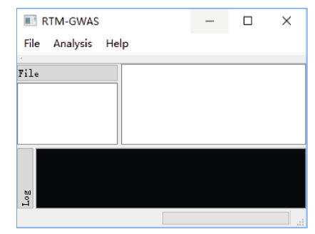
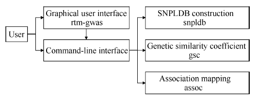
我们编制了实现RTM-GWAS方法的计算程序, 可从项目网站https://github.com/njau-sri/rtm-gwas/下载使用。RTM-GWAS计算程序使用C++编程语言实现, 可运行于Microsoft Windows、Linux和Mac OS X等主流操作系统平台。借助针对不同处理器优化的高性能线性代数运算库, RTM-GWAS计算程序具有较高的计算效率。RTM-GWAS计算程序拥有交互友好的图形用户界面和用于批量任务的命令行界面(图1)。RTM-GWAS计算程序构架如图2所示, 由SNPLDB标记构建、遗传相似系数矩阵计算和关联分析三个核心模块组成, 用户可分别通过图形界面或命令行界面进行相应的计算分析, 详细操作说明见https://github.com/njau-sri/rtm-gwas/wiki。RTM- GWAS计算程序输出结果以文本文件存储, 可使用任意本文编辑软件查看输出结果。图1
 新窗口打开|下载原图ZIP|生成PPT
图1RTM-GWAS方法计算程序图形用户界面
Fig. 1Graphical user interface of the RTM-GWAS analytical program
图2
 新窗口打开|下载原图ZIP|生成PPT
图2RTM-GWAS方法计算程序构架
斜体文字为相应功能的二进制程序名称。
Fig. 2Framework of the RTM-GWAS analytical program
The characters in italic type are names of binary program.
2.1 数据文件格式
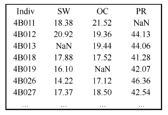
分子标记数据采用国际通用的VCF文件格式 (https://github.com/samtools/hts-specs), 该文件格式适用于各种标记类型, 也是软件支持较为广泛的标记数据格式之一, 因此便于不同软件间协同分析。表型数据是空格或制表符作为分隔符的文本文件, 图3所示为3个性状的表型数据文件(仅显示前7个材料), 文件第1行为列名, 从第2行开始每行表示一条观测值。其中, 第1列为个体编号, 其余列为不同性状观测值, 第1列的列名可以任意, 其余列名表示不同性状的名称。观测值必须使用数值格式记录, 缺失值可使用“NaN”、“?”、“NA”或“.”表示。对于多环境随机区组设计试验数据, 文件必须包含指示环境和区组因子的数据列, 列名必须是“_ENV_”和“_BLK_”, 分别表示环境和区组指示变量。图3
 新窗口打开|下载原图ZIP|生成PPT
图3表型数据文件格式
Indiv表示个体/材料名称列名; SW、OC、PR为性状名称; NaN表示缺失值。
Fig. 3File format of phenotype data
Indiv represents the name of column containing individual/ accession labels; SW, OC, PR are trait names; NaN represents missing value.
2.2 SNPLDB标记构建
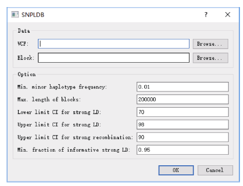
指定VCF格式的全基因组SNP基因型数据文件后即可开始计算, 计算程序将输出VCF格式的SNPLDB标记基因型数据文件、标记位点等位变异编码信息以及基因组组块统计信息。计算程序默认单倍型频率(Min. minor haplotype frequency)≥0.01, 区段最大长度(Max. length of blocks)为200 kb, 建议设置为群体连锁不平衡半衰距离。构建SNPLDB的3组核心参数是, LD置信区间阈值(Lower/Upper limit CI for strong LD), 在定义强LD时对LD置信上下限均作最小范围要求, 即要求下限 >70、上限 >98; 强重组置信区间阈值(Upper limit CI for strong recombination)上限<90; 区段内有效强LD占比(Min. fraction of informative strong LD) > 0.95 (图4)。图4
 新窗口打开|下载原图ZIP|生成PPT
图4SNPLDB标记构建对话框
VCF指以VCF格式存储的基因型数据文件路径; Min.: 最小值; Max.: 最大值; CI: 置信区间。
Fig. 4Program dialog for SNPLDB construction
VCF represents the VCF genotype file path; Min.: minimum;Max.: maximum; CI: confidence interval.
2.3 遗传相似系数计算
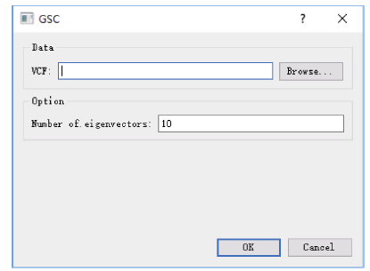
指定构建的SNPLDB标记文件(VCF格式)后即可计算, 计算程序将输出遗传相似系数矩阵及其特征向量, 默认输出前10个特征向量。其中输出的特征向量文件将作为关联分析的协变量用于群体结构矫正(图5)。图5
 新窗口打开|下载原图ZIP|生成PPT
图5遗传相似系数计算对话框
VCF指以VCF格式存储的基因型数据文件路径。
Fig. 5Program dialog for genetic similarity coefficient calculation
VCF represents the VCF genotype file path.
2.4 两阶段多位点关联分析
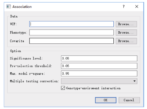
关联分析功能对话框需要指定SNPLDB标记基因型数据文件(VCF格式)、数量性状表型观测数据以及用于群体结构矫正的协变量(SNPLDB遗传相似系数矩阵特征向量)数据文件, 计算程序将输出与性状关联的SNPLDB标记位点、多位点模型方差分析、位点等位基因效应估计等结果文件。计算程序默认用于检测QTL的显著水平(significance level)为0.05, 建议设为0.01或0.05。用于标记初步筛选(第一阶段)的阈值默认为0.05, 一般不建议修改。为防止模型过度拟合, 计算默认设置了模型表型变异解释率上限(Max. model r-square)为0.95, 建议设为性状遗传率估计值(图6)。关联分析程序也支持多重测验矫正(multiple testing correction), 包括Bonferroni (BON)和FDR两种方法, 通常矫正后检测的位点也包含于未矫正的结果。另外, 关联分析程序还支持多环境试验原始表型数据的计算, 计算程序默认能够检测QTL与环境互作效应, 但是当基因型与环境互作方差相对较小时, 可以排除QTL与环境互作效应(genotype-environment interaction), 以降低统计模型的复杂度。图6
 新窗口打开|下载原图ZIP|生成PPT
图6关联分析功能对话框
VCF指以VCF格式存储的基因型数据文件路径; Max.: 最大值; r-square: 模型决定系数。
Fig. 6Program dialog for association analysis
VCF represents the VCF genotype file path; Max.: maximum; r-square: coefficient of determination.
3 RTM-GWAS在大豆资源群体中的应用
以下以中国栽培大豆资源群体株高试验结果的全基因组关联分析为例说明RTM-GWAS方法的应用, 详细应用可参考已发表的文献[18,19,20,21]。3.1 试验数据
参试的723份栽培大豆来自中国大豆种质资源群体, 分别于2013年和2014年进行田间试验, 采用随机区组试验设计, 设3次重复, 品种成熟后测量株高。试验群体株高变异范围15~165 cm, 平均62.78 cm, 变异系数41.57%。2年试验株高误差变异系数14.33%, 遗传率0.921, 基因与环境互作遗传率0.049。基因型数据来自用RAD-seq (restriction site-associated DNA sequencing)技术对该群体进行的基因型分型[18]。通过序列比对将测序片段比对到大豆Williams 82参考基因组并进行SNP鉴别, SNP质量控制采用的过滤标准为缺失和杂合率小于或等于20%, 最小等位基因频率大于或等于1%。最后使用fastPHASE软件[26]对SNP缺失基因型进行填补, 获得了145 558个覆盖全基因组的高质量SNP标记。3.2 利用RTM-GWAS检测株高全基因组QTL
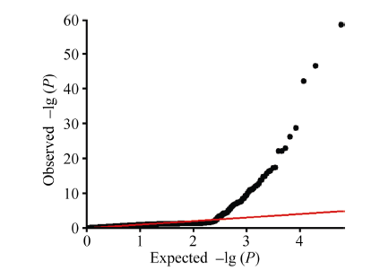
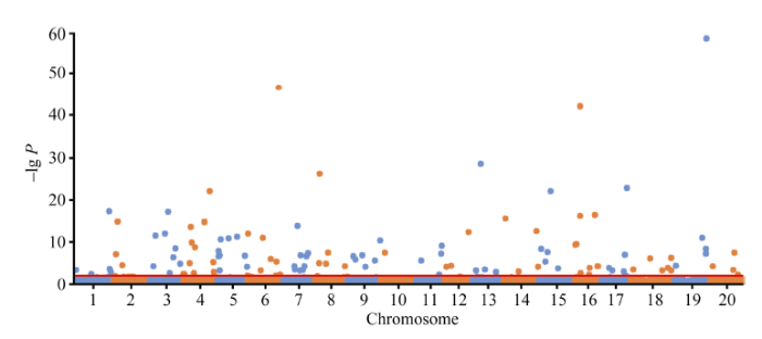
首先, 基于全基因组145 558个SNP标记, 利用RTM-GWAS计算程序进行SNPLDB标记构建, 采用程序默认参数。程序输出了36 952个SNPLDB标记的VCF格式基因型数据文件, 用于后续所有分析。其次, 基于构建好的SNPLDB标记, 利用RTM- GWAS计算程序计算群体内个体间的遗传相似系数矩阵, 并提取特征值最大的前10个特征向量作为控制群体结构的协变量。最后, 基于大豆株高表型原始观测值、SNPLDB标记数据以及遗传相似系数矩阵特征向量, 利用RTM-GWAS计算程序关联分析功能对大豆株高进行全基因组QTL检测并估计QTL等位基因的效应。QTL检测的显著水平设为0.01, 模型解释率上限设置为0.921, 其他参数保持默认。关联分析程序输出5个结果文件, 关联标记位点名称文件assoc.out.loc、I型模型方差分析文件assoc.out.aov1、III型模型方差分析文件assoc.out. aov3、等位基因效应估计文件assoc.out.est、标记位点统计检验概率值(P-value)文件assoc.out.ps。基于所有标记位点关联测验P值结果数据文件, 可使用绘图软件, 如R软件(http://www.r-project. org/), 绘制Q-Q图(图7)和Manhattan图(图8)。用RTM-GWAS方法共检测到114个SNPLDB位点与株高性状关联, 根据方差分析结果数据文件, 其中10个位点主效不显著, 63个位点与环境互作效应不显著。104个主效显著的位点总表型变异解释率为78.103%, 51个显著的位点与环境互作效应总表型变异解释率为10.312%, 其中有21个位点主效表型变异解释率高于1%, 将结果进一步整理为表1, 所有位点关联结果详见附件表1。RTM-GWAS分析程序不会输出位点贡献率, 但可以根据输出的平方和分解计算位点贡献率, 即位点平方和占总平方和的比例。
图7
 新窗口打开|下载原图ZIP|生成PPT
图7大豆株高全基因组关联分析Q-Q图
Fig. 7Quantile-Quantile plot of genome-wide association study of soybean plant height
Table 1
表1
表1大豆株高显著关联的大效应SNPLDB标记位点
Table 1
| SNPLDB | 染色体 Chromosome | 位置 Position | Model a | QTL | QTL×Env. b | ||
|---|---|---|---|---|---|---|---|
| -lg P | -lg P | R2 (%) | -lg P | R2 (%) | |||
| LDB_19_44964630 | 19 | 44964630-45029584 | 58.26 | 206.01 | 7.361 | 52.86 | 1.693 |
| LDB_6_44183574 | 6 | 44183574-44281248 | 46.46 | 199.50 | 7.359 | 11.64 | 0.495 |
| LDB_16_8004288 | 16 | 8004288-8203845 | 42.01 | 171.86 | 6.140 | 6.15 | 0.280 |
| LDB_13_11539212 | 13 | 11539212-11625990 | 28.64 | 120.36 | 4.091 | 0.66 | 0.053 |
| LDB_17_36474880 | 17 | 36474880-36494652 | 22.81 | 96.33 | 3.229 | 0.80 | 0.059 |
| LDB_4_37782684 | 4 | 37782684-37923093 | 22.06 | 83.36 | 2.809 | 3.39 | 0.170 |
| LDB_8_7075139 | 8 | 7075139-7077091 | 26.19 | 81.67 | 2.616 | 16.09 | 0.505 |
| LDB_3_26698545 | 3 | 26698545-26898267 | 17.24 | 68.85 | 2.423 | 4.56 | 0.261 |
| LDB_15_16773982 | 15 | 16773982-16774010 | 22.09 | 72.65 | 2.273 | 5.22 | 0.154 |
| LDB_16_28838874 | 16 | 28838874-28868118 | 16.44 | 56.11 | 1.887 | 1.01 | 0.077 |
| LDB_4_11093449 | 4 | 11093449-11192120 | 13.61 | 51.18 | 1.800 | 3.13 | 0.195 |
| LDB_2_5863888 | 2 | 5863888-5979031 | 14.88 | 47.63 | 1.493 | 1.06 | 0.042 |
| LDB_16_7494681 | 16 | 7494681 | 16.21 | 48.32 | 1.440 | 1.04 | 0.018 |
| LDB_1_50277902 | 1 | 50277902 | 17.34 | 47.47 | 1.413 | 8.98 | 0.239 |
| LDB_14_2467475 | 14 | 2467475 | 15.57 | 45.66 | 1.356 | 0.88 | 0.014 |
| LDB_4_29936477 | 4 | 29936477-29950803 | 14.74 | 38.98 | 1.217 | 5.63 | 0.186 |
| LDB_3_22147965 | 3 | 22147965-22342699 | 11.98 | 32.08 | 1.209 | 11.34 | 0.516 |
| LDB_7_20253563 | 7 | 20253563-20451607 | 13.83 | 36.68 | 1.174 | 2.68 | 0.108 |
| LDB_14_46095634 | 14 | 46095634-46106570 | 12.67 | 35.50 | 1.076 | 0.28 | 0.008 |
| LDB_3_8197776 | 3 | 8197776-8202466 | 11.51 | 32.01 | 1.026 | 1.05 | 0.052 |
| LDB_6_22108685 | 6 | 22108685-22191360 | 10.97 | 28.35 | 1.004 | 5.03 | 0.241 |
新窗口打开|下载CSV
全国从东北到西南大豆资源的株高在南京表现出有114个位点的差异, 年份间有波动。关联的114个SNPLDB位点共有442个等位变异, 其中主效显著的104个位点共有417个等位变异。由于本研究大豆株高遗传基础以主效位点为主, 简便起见, 本文则以主效位点为例进行后续分析, 如要考虑特定环境的分析, 可将位点主效应与相应环境互作效应相加后再进行分析。根据主效显著的104个位点效应估计结果, 等位变异效应范围为-43.55~ +38.26, 结合群体SNPLDB基因型, 可进一步将等位变异效应整理为位点×材料(104×417)的QTL-allele矩阵作为群体株高性状的遗传构成(图9), 可以进一步使用绘图软件将该矩阵可视化(图10)。
图8
 新窗口打开|下载原图ZIP|生成PPT
图8大豆株高全基因组关联分析Manhattan图
Fig. 8Manhattan plot of genome-wide association study of soybean plant height
图9
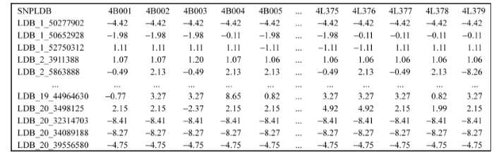 新窗口打开|下载原图ZIP|生成PPT
图9大豆株高主效QTL-allele矩阵数据文件
行表示104个主效显著的株高关联位点, 列表示723份栽培大豆材料, 数据为104×723的主效位点等位基因效应矩阵。
Fig. 9QTL-allele matrix data file of main effect
Rows represent the 104 loci and columns represent the 723 accessions, the data are allele effects and presented in 104×723 matrix.
图10
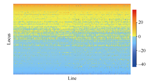 新窗口打开|下载原图ZIP|生成PPT
图10大豆株高QTL-allele可视化矩阵
Fig. 10Graphical representation of the QTL-allele matrix of soybean plant height
3.3 基于QTL-allele矩阵的优化组合设计
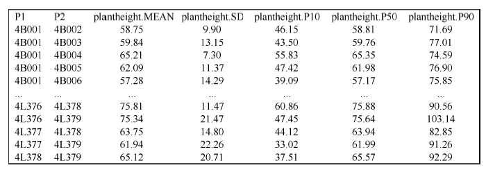
对于723个材料所有可能261 003个单交组合, 通过F1连续自交分别模拟产生2000个纯系后代基因型, 依据包括104个位点效应的株高QTL-allele矩阵计算所有QTL基因型值总和, 作为后代基因型值预测值。亲本i和亲本j组合的表型预测值为 yij = gij + (yi - gi + yj - gj)/2, 其中gij为组合后代基因型预测值, yi和yj分别为双亲表型观测值, gi和gj分别为双亲基因型值预测值。所有模拟计算通过编制的计算程序Cross (https://github.com/njau-sri/cross)完成, 计算程序将输出所有单交组合后代纯合群体的株高性状描述统计数据(图11), 可根据实际需求在计算程序中设置用于筛选优化组合的百分位数统计量, 计算程序默认输出第1 (最小值)、25 (Q1)、50 (中位数)、75 (Q3)、100 (最大值)百分位数, 本文设置第10、第50、第90百分位数作为选择依据。后代纯合群体第10、第50、第90百分位数使用其他绘图软件绘制的散点图, 可以看出第10、第90百分位数均有超亲组合出现(图12)。以高杆大豆育种为例, 按照第90百分位数筛选优化组合, 可筛选出101个亲本组合预测株高大于165 cm的组合, 详见附件表2, 其中预测株高大于180 cm的亲本组合有8个(表2), 预测株高最高可达183 cm, 相比亲本株高165 cm提高了10.9% (18 cm)。图11
 新窗口打开|下载原图ZIP|生成PPT
图11株高性状所有亲本组合后代预测结果文件
P1、P2分别表示单交组合的2个亲本; MEAN、SD分别表示组合纯合后代群体株高平均数和标准差; P10、P50、P90分别表示组合纯合后代群体株高第10、第50、第90百分位数。
Fig. 11Prediction result file of plant height for all possible single crosses
P1 and P2 are labels of parental accessions; MEAN and SD indicate the mean and standard deviation of homozygous progeny population; P10, P50, and P90 are 10-th, 50-th, and 90-th percentiles of homozygous progeny population.
图12
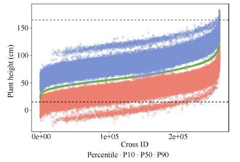 新窗口打开|下载原图ZIP|生成PPT
图12株高性状所有亲本组合后代预测结果可视化
虚线表示亲本群体株高变异范围(15~165 cm)。
Fig. 12Graphical representation of the prediction result of plant height for all possible single crosses
Dotted lines indicate the range (15-165 cm) of plant height in parental population.
4 讨论
4.1 RTM-GWAS方法功效
和以往GWAS方法专注于个别主效QTL的检测不同, RTM-GWAS方法能够相对全面地解析植物种质/育种群体数量性状的QTL体系。首先, 以往GWAS均基于仅有的2个等位变异的SNP标记, 而无法检测一个遗传位点上多个复等位基因。对于一个遗传位点上存在多个复等位基因的情况, 单个SNP标记测验仅能解释遗传位点的部分遗传变异, 理论上统计功效自然会偏低, 从而会降低GWAS检测功效。RTM-GWAS方法通过构建具有复等位变异的SNPLDB标记来匹配具有复等位基因的位点, 理论上使得GWAS更适用于存在广泛复等位基因的种质资源群体。其次, 以往基于单位点模型的GWAS方法由于忽略了其他位点的影响, 可能导致较高假阳性的检测结果。然而由于GWAS通常基于全基因高密度分子标记, 直接拟合多位点模型将导致计算量过大, 影响计算效率。RTM-GWAS方法结合两阶段分析策略和多位点模型, 不仅能够同时拟合多个具有不等数目等位基因的遗传位点, 提高了检测功效, 还大幅降低了计算量, 提高了计算效率, 使得RTM-GWAS方法可以应用于大规模GWAS数据的分析。植物中表型鉴定试验通常是多个环境的重复试验, 以往主流GWAS方法通常不支持多环境表型数据联合分析, 而是将基因型多环境调整平均数作为GWAS分析的表型, 不仅无法分析主效QTL与环境互作效应, 更无法检测仅有互作效应而没有主效的QTL。RTM-GWAS方法计算程序支持多环境随机区组试验设计的原始表型数据分析, 能够同时拟合主效和非主效QTL与环境互作效应, 检测结果更加全面。另外, 模拟分析显示应用RTM-GWAS方法的样本容量需要足够大(例如, >400)且性状遗传率也应较高(例如, >0.8), 因此表型鉴定需要进行合理的试验设计以及精确的试验操作[18]。
4.2 RTM-GWAS方法应用前景
RTM-GWAS方法不仅适用于种质资源群体, 也适用于多亲本的NAM群体[21]。RTM-GWAS方法通过构建具有亲本单倍型的SNPLDB标记, 将NAM群体内不同RIL群体视为一个自然的整体, 每个标记位点具有不同的等位变异类型, 而不是像以往分析将RIL群体视为彼此独立的群体[27]。由于NAM群体的遗传设计特点, 其群体结构已知, 因此RTM-GWAS方法可以较好地控制群体结构, 从而获得较高的检测功效和较低的假发现率。潘丽媛等(未发表)也将RTM-GWAS方法用于大豆RIL群体的QTL定位, 比较结果显示, RTM-GWAS方法不仅覆盖了复合区间作图法的定位结果, 还检测到更多的已报道微效QTL。由于RTM-GWAS方法是对标记位点进行检验, 无法对标记区间内的任意位置进行检验, 因此NAM和RIL群体必须进行全基因组SNP标记鉴定才可能进行全基因组QTL的检测。RTM-GWAS方法较高的检测功效使得其检测结果可以全面反映群体数量性状遗传构成, 从而能够进一步从全基因组QTL水平对育种亲本组合进行潜力预测及优化组合设计, 在实际育种前直接对QTL进行育种选择。基于RTM-GWAS方法获得的QTL-allele矩阵, 可通过设计分子标记进一步应用于双亲后代选择, 从而提高选择效率、缩短育种周期。基于全基因组QTL的组合预测和后代选择是对QTL直接选择, 不同于传统全基因组选择(genomic selection, GS)方法对全基因组分子标记进行选择[28]。传统GS需要对选择世代进行全基因组分子标记测定, 目前对于植物育种花费十分高昂。GS训练群体与选择群体的遗传关系以及预测模型构建方法会直接影响选择效率, 主要应用于组合后代的选择, 把GS直接应用于优化组合设计会由于需要对组合后代进行全基因组标记模拟, 进而导致难以接受的计算量。
此外, 基于全基因组QTL及其等位基因构成信息, 还可以从QTL水平上刻画群体遗传特征, 进行群体分化以及群体间进化关系的研究。例如Meng等[20]对RTM-GWAS检测的44个异黄酮含量QTL进行生态区基因频率的分析结果显示, 84.1% (37个)的位点基因频率在生态区间存在显著差异, 而在全基因组29 119个SNPLDB标记水平上, 则只有50.6% (14 735个)的位点基因频率在生态区间存在显著差异, 进一步说明了异黄酮含量遗传构成在生态区上发生了分化。
5 结论
本研究提出的RTM-GWAS方法通过将多个相邻且紧密连锁的SNP分组, 构建具有复等位变异的SNPLDB标记, 然后采用两阶段分析策略, 基于多位点模型检测全基因组QTL及其复等位变异。和以往GWAS方法相比, RTM-GWAS方法能较充分地检测出QTL及其相应的复等位变异, 并能有效地控制假阳性。由其结果建立的QTL-allele矩阵代表了试验群体中所研究性状的全部遗传构成, 不仅可用于设计最优基因型的遗传组成, 预测最优杂交组合, 还能用于群体遗传和特有与新生等位变异的研究。Supplementary table 1
附表1
附表1大豆株高显著关联的SNPLDB标记位点
Supplementary table 1
| SNPLDB | 染色体 Chromosome | 位置 Position | Model a | QTL | QTL×Env. b | ||
|---|---|---|---|---|---|---|---|
| -lg P | -lg P | R2 (%) | -lg P | R2 (%) | |||
| LDB_19_44964630 | 19 | 44964630-45029584 | 58.26 | 206.01 | 7.361 | 52.86 | 1.693 |
| LDB_6_44183574 | 6 | 44183574-44281248 | 46.46 | 199.50 | 7.359 | 11.64 | 0.495 |
| LDB_16_8004288 | 16 | 8004288-8203845 | 42.01 | 171.86 | 6.140 | 6.15 | 0.280 |
| LDB_13_11539212 | 13 | 11539212-11625990 | 28.64 | 120.36 | 4.091 | 0.66 | 0.053 |
| LDB_17_36474880 | 17 | 36474880-36494652 | 22.81 | 96.33 | 3.229 | 0.80 | 0.059 |
| LDB_4_37782684 | 4 | 37782684-37923093 | 22.06 | 83.36 | 2.809 | 3.39 | 0.170 |
| LDB_8_7075139 | 8 | 7075139-7077091 | 26.19 | 81.67 | 2.616 | 16.09 | 0.505 |
| LDB_3_26698545 | 3 | 26698545-26898267 | 17.24 | 68.85 | 2.423 | 4.56 | 0.261 |
| LDB_15_16773982 | 15 | 16773982-16774010 | 22.09 | 72.65 | 2.273 | 5.22 | 0.154 |
| LDB_16_28838874 | 16 | 28838874-28868118 | 16.44 | 56.11 | 1.887 | 1.01 | 0.077 |
| LDB_4_11093449 | 4 | 11093449-11192120 | 13.61 | 51.18 | 1.800 | 3.13 | 0.195 |
| LDB_2_5863888 | 2 | 5863888-5979031 | 14.88 | 47.63 | 1.493 | 1.06 | 0.042 |
| LDB_16_7494681 | 16 | 7494681 | 16.21 | 48.32 | 1.440 | 1.04 | 0.018 |
| LDB_1_50277902 | 1 | 50277902 | 17.34 | 47.47 | 1.413 | 8.98 | 0.239 |
| LDB_14_2467475 | 14 | 2467475 | 15.57 | 45.66 | 1.356 | 0.88 | 0.014 |
| LDB_4_29936477 | 4 | 29936477-29950803 | 14.74 | 38.98 | 1.217 | 5.63 | 0.186 |
| LDB_3_22147965 | 3 | 22147965-22342699 | 11.98 | 32.08 | 1.209 | 11.34 | 0.516 |
| LDB_7_20253563 | 7 | 20253563-20451607 | 13.83 | 36.68 | 1.174 | 2.68 | 0.108 |
| LDB_14_46095634 | 14 | 46095634-46106570 | 12.67 | 35.50 | 1.076 | 0.28 | 0.008 |
| LDB_3_8197776 | 3 | 8197776-8202466 | 11.51 | 32.01 | 1.026 | 1.05 | 0.052 |
| LDB_6_22108685 | 6 | 22108685-22191360 | 10.97 | 28.35 | 1.004 | 5.03 | 0.241 |
| LDB_6_1271502 | 6 | 1271502-1275159 | 12.04 | 32.96 | 0.997 | 0.61 | 0.018 |
| LDB_12_34374105 | 12 | 34374105 | 12.35 | 32.82 | 0.956 | 0.40 | 0.005 |
| LDB_5_27543725 | 5 | 27543725-27547377 | 11.25 | 27.31 | 0.851 | 1.50 | 0.056 |
| LDB_5_4082209 | 5 | 4082209-4121721 | 10.60 | 26.74 | 0.834 | 2.20 | 0.079 |
| LDB_4_16641482 | 4 | 16641482-16839772 | 8.72 | 22.21 | 0.786 | 2.84 | 0.150 |
| LDB_19_39240844 | 19 | 39240844-39276967 | 11.01 | 23.49 | 0.759 | 5.16 | 0.188 |
| LDB_5_15648588 | 5 | 15648588 | 10.85 | 25.48 | 0.731 | 0.14 | 0.001 |
| LDB_4_12429588 | 4 | 12429588-12605113 | 9.93 | 20.00 | 0.715 | 6.46 | 0.276 |
| LDB_9_45791340 | 9 | 45791340 | 10.33 | 22.42 | 0.638 | 0.56 | 0.008 |
| LDB_3_36428638 | 3 | 36428638-36469336 | 8.56 | 19.15 | 0.624 | 1.44 | 0.066 |
| LDB_16_2807415 | 16 | 2807415-2827492 | 9.48 | 17.29 | 0.588 | 6.02 | 0.231 |
| SNPLDB | 染色体 Chromosome | 位置 Position | Model a | QTL | QTL×Env. b | ||
| -lg P | -lg P | R2 (%) | -lg P | R2 (%) | |||
| LDB_11_35694247 | 11 | 35694247-35698584 | 9.13 | 18.50 | 0.553 | 0.30 | 0.009 |
| LDB_7_35303124 | 7 | 35303124-35327231 | 7.34 | 15.83 | 0.542 | 1.43 | 0.076 |
| LDB_15_12007768 | 15 | 12007768-12011501 | 7.68 | 16.51 | 0.492 | 0.18 | 0.005 |
| LDB_7_32985427 | 7 | 32985427-33184712 | 6.68 | 13.54 | 0.489 | 0.74 | 0.057 |
| LDB_2_3911388 | 2 | 3911388-3928107 | 7.14 | 14.07 | 0.466 | 1.34 | 0.062 |
| LDB_9_20673268 | 9 | 20673268-20692609 | 6.87 | 13.82 | 0.436 | 0.33 | 0.016 |
| LDB_16_1151749 | 16 | 1151749 | 9.34 | 15.53 | 0.432 | 4.63 | 0.115 |
| LDB_19_44669655 | 19 | 44669655-44754287 | 8.40 | 13.62 | 0.430 | 7.17 | 0.233 |
| LDB_5_907001 | 5 | 907001-907042 | 7.84 | 15.21 | 0.423 | 0.13 | 0.001 |
| LDB_9_8062600 | 9 | 8062600-8116659 | 6.60 | 11.79 | 0.374 | 1.12 | 0.044 |
| LDB_8_19152075 | 8 | 19152075-19152100 | 7.48 | 13.34 | 0.367 | 0.92 | 0.015 |
| LDB_10_5777915 | 10 | 5777915-5798626 | 7.46 | 10.73 | 0.362 | 5.67 | 0.204 |
| LDB_19_44550587 | 19 | 44550587-44558289 | 7.30 | 11.07 | 0.352 | 3.42 | 0.117 |
| LDB_20_34089188 | 20 | 34089188 | 7.57 | 12.42 | 0.340 | 1.11 | 0.020 |
| LDB_5_2803587 | 5 | 2803587 | 6.90 | 12.30 | 0.336 | 0.35 | 0.004 |
| LDB_8_16373446 | 8 | 16373446-16420876 | 4.96 | 10.50 | 0.334 | 0.32 | 0.016 |
| LDB_18_57452705 | 18 | 57452705-57457239 | 6.26 | 10.95 | 0.325 | 0.33 | 0.010 |
| LDB_7_25096830 | 7 | 25096830 | 6.89 | 11.75 | 0.320 | 0.36 | 0.004 |
| LDB_9_38183930 | 9 | 38183930-38268800 | 5.66 | 7.74 | 0.319 | 4.07 | 0.194 |
| LDB_12_9936416 | 12 | 9936416-9994538 | 4.45 | 8.40 | 0.307 | 0.79 | 0.050 |
| LDB_3_33432777 | 3 | 33432777-33462071 | 6.40 | 9.52 | 0.305 | 1.19 | 0.046 |
| LDB_5_1382138 | 5 | 1382138 | 6.66 | 10.46 | 0.283 | 0.70 | 0.010 |
| LDB_6_33023321 | 6 | 33023321 | 6.03 | 10.09 | 0.272 | 0.39 | 0.004 |
| LDB_11_35162270 | 11 | 35162270 | 7.31 | 10.07 | 0.271 | 5.10 | 0.128 |
| LDB_18_27478142 | 18 | 27478142 | 6.16 | 10.06 | 0.271 | 0.46 | 0.006 |
| LDB_17_33708118 | 17 | 33708118-33815088 | 7.03 | 7.77 | 0.251 | 6.96 | 0.226 |
| LDB_5_38350041 | 5 | 38350041-38432356 | 6.76 | 7.19 | 0.233 | 5.51 | 0.182 |
| LDB_11_6370581 | 11 | 6370581-6486015 | 5.64 | 6.03 | 0.231 | 3.87 | 0.161 |
| LDB_16_31959033 | 16 | 31959033-31999963 | 4.27 | 7.11 | 0.231 | 0.46 | 0.021 |
| LDB_18_44942878 | 18 | 44942878-45064511 | 3.28 | 5.38 | 0.225 | 0.48 | 0.044 |
| LDB_2_12669763 | 2 | 12669763-12684207 | 4.48 | 5.69 | 0.204 | 1.20 | 0.057 |
| LDB_6_41523578 | 6 | 41523578 | 5.41 | 7.71 | 0.203 | 0.81 | 0.013 |
| LDB_17_15782164 | 17 | 15782164-15845977 | 3.22 | 3.92 | 0.189 | 0.78 | 0.066 |
| LDB_4_42809656 | 4 | 42809656-42809670 | 5.27 | 5.79 | 0.171 | 2.76 | 0.081 |
| LDB_9_25244209 | 9 | 25244209 | 4.20 | 6.56 | 0.170 | 0.20 | 0.002 |
| LDB_3_43245339 | 3 | 43245339 | 4.91 | 6.56 | 0.170 | 0.25 | 0.002 |
| LDB_15_9202681 | 15 | 9202681 | 5.40 | 6.24 | 0.160 | 3.37 | 0.079 |
| LDB_20_3498125 | 20 | 3498125-3691528 | 4.33 | 3.82 | 0.159 | 2.93 | 0.129 |
| LDB_17_11367127 | 17 | 11367127-11382009 | 3.93 | 4.76 | 0.159 | 1.85 | 0.068 |
| LDB_17_32520275 | 17 | 32520275-32552871 | 3.03 | 2.75 | 0.147 | 1.72 | 0.107 |
| LDB_16_32918946 | 16 | 32918946 | 4.25 | 5.59 | 0.142 | 1.19 | 0.022 |
| LDB_12_3456148 | 12 | 3456148 | 4.19 | 5.44 | 0.137 | 1.63 | 0.033 |
| LDB_8_6056566 | 8 | 6056566 | 5.03 | 5.37 | 0.136 | 1.85 | 0.038 |
| LDB_4_9550687 | 4 | 9550687-9550998 | 5.03 | 4.57 | 0.135 | 3.77 | 0.111 |
| SNPLDB | 染色体 Chromosome | 位置 Position | Model a | QTL | QTL×Env. b | ||
| -lg P | -lg P | R2 (%) | -lg P | R2 (%) | |||
| LDB_5_2285265 | 5 | 2285265-2285296 | 3.31 | 4.50 | 0.133 | 1.00 | 0.030 |
| LDB_15_27523398 | 15 | 27523398-27723343 | 3.84 | 3.02 | 0.132 | 3.47 | 0.147 |
| LDB_13_4599736 | 13 | 4599736 | 3.30 | 4.78 | 0.119 | 0.10 | 0.000 |
| LDB_9_10672160 | 9 | 10672160-10831207 | 5.87 | 4.01 | 0.118 | 6.77 | 0.200 |
| LDB_1_50652928 | 1 | 50652928-50669137 | 3.70 | 2.97 | 0.117 | 2.84 | 0.113 |
| LDB_18_52669179 | 18 | 52669179 | 3.92 | 4.71 | 0.117 | 1.55 | 0.031 |
| LDB_6_18845190 | 6 | 18845190 | 3.30 | 4.49 | 0.111 | 1.13 | 0.020 |
| LDB_13_17681170 | 13 | 17681170 | 3.51 | 4.26 | 0.104 | 0.25 | 0.002 |
| LDB_4_15008106 | 4 | 15008106-15030261 | 2.72 | 2.85 | 0.099 | 1.58 | 0.059 |
| LDB_20_39556580 | 20 | 39556580 | 2.34 | 3.88 | 0.094 | 0.61 | 0.009 |
| LDB_16_20099141 | 16 | 20099141 | 2.27 | 3.87 | 0.093 | 0.18 | 0.001 |
| LDB_14_20541667 | 14 | 20541667 | 3.05 | 3.80 | 0.091 | 0.56 | 0.008 |
| LDB_15_3242880 | 15 | 3242880 | 8.41 | 3.74 | 0.090 | 13.78 | 0.380 |
| LDB_1_52750312 | 1 | 52750312 | 2.93 | 3.72 | 0.089 | 0.25 | 0.002 |
| LDB_16_21247996 | 16 | 21247996 | 3.85 | 3.59 | 0.085 | 1.90 | 0.040 |
| LDB_3_28458666 | 3 | 28458666 | 2.67 | 3.26 | 0.076 | 0.89 | 0.015 |
| LDB_18_3933946 | 18 | 3933946 | 3.53 | 3.14 | 0.073 | 1.65 | 0.033 |
| LDB_7_15901391 | 7 | 15901391-15903281 | 4.33 | 2.93 | 0.067 | 4.15 | 0.101 |
| LDB_19_2090261 | 19 | 2090261-2090611 | 4.43 | 2.92 | 0.067 | 4.40 | 0.108 |
| LDB_7_27922333 | 7 | 27922333-28121779 | 3.45 | 1.47 | 0.067 | 3.33 | 0.129 |
| LDB_5_41679020 | 5 | 41679020 | 4.15 | 2.90 | 0.067 | 3.78 | 0.091 |
| LDB_18_57497434 | 18 | 57497434-57500329 | 3.29 | 2.79 | 0.064 | 1.07 | 0.019 |
| LDB_4_571693 | 4 | 571693 | 2.40 | 2.63 | 0.059 | 1.66 | 0.034 |
| LDB_6_46436793 | 6 | 46436793-46436833 | 2.30 | 2.56 | 0.057 | 1.05 | 0.018 |
| LDB_20_32314703 | 20 | 32314703 | 3.45 | 2.40 | 0.053 | 2.98 | 0.069 |
| LDB_8_42752500 | 8 | 42752500 | 4.23 | 2.40 | 0.053 | 3.74 | 0.090 |
| LDB_4_43757706 | 4 | 43757706 | 2.86 | 2.40 | 0.053 | 2.38 | 0.052 |
| LDB_11_31994374 | 11 | 31994374-31994436 | 2.28 | 2.31 | 0.051 | 0.76 | 0.012 |
| LDB_4_1643625 | 4 | 1643625-1744093 | 2.39 | 1.65 | 0.049 | 3.06 | 0.090 |
| LDB_16_8204099 | 16 | 8204099 | 2.68 | 2.08 | 0.044 | 1.63 | 0.033 |
| LDB_13_33478164 | 13 | 33478164 | 2.85 | 1.79 | 0.037 | 3.21 | 0.075 |
| LDB_14_48799491 | 14 | 48799491-48799496 | 4.12 | 1.20 | 0.035 | 4.55 | 0.134 |
| LDB_7_16630442 | 7 | 16630442 | 3.58 | 1.55 | 0.031 | 3.76 | 0.090 |
| LDB_3_5207322 | 3 | 5207322 | 4.23 | 1.45 | 0.028 | 4.94 | 0.123 |
| LDB_7_23869970 | 7 | 23869970 | 3.28 | 1.26 | 0.024 | 3.41 | 0.081 |
| LDB_1_3351751 | 1 | 3351751 | 3.42 | 0.89 | 0.015 | 3.41 | 0.081 |
| LDB_7_30278846 | 7 | 30278846 | 4.23 | 0.60 | 0.008 | 6.12 | 0.157 |
| LDB_1_24895878 | 1 | 24895878 | 2.40 | 0.36 | 0.004 | 3.14 | 0.073 |
| Total | 114 | 104 c | 78.103 | 51 d | 10.312 | ||
新窗口打开|下载CSV
Supplementary table 2
附表2
附表2高杆大豆育种化组合设计
Supplementary table 2
| 亲本 Parent | 组合 Cross | |||||||
|---|---|---|---|---|---|---|---|---|
| P1 | P2 | Y1 | Y2 | 平均数 Mean | 标准差 SD | P10 | P50 | P90 |
| 4L060 | 4L311 | 136.3 | 132.3 | 135.4 | 36.1 | 87.5 | 135.5 | 183.3 |
| 4L119 | 4L361 | 125.0 | 138.6 | 132.3 | 37.2 | 81.6 | 131.8 | 182.2 |
| 4L213 | 4L361 | 127.6 | 138.6 | 133.5 | 35.9 | 84.4 | 134.4 | 181.3 |
| 4L060 | 4L119 | 136.3 | 125.0 | 130.6 | 37.4 | 80.5 | 130.3 | 180.8 |
| 4L054 | 4L060 | 133.5 | 136.3 | 134.6 | 33.4 | 91.3 | 133.7 | 180.8 |
| 4L311 | 4L361 | 132.3 | 138.6 | 134.3 | 35.2 | 87.7 | 134.4 | 180.7 |
| 4L054 | 4L361 | 133.5 | 138.6 | 136.3 | 33.6 | 92.8 | 135.3 | 180.7 |
| 4L060 | 4L371 | 136.3 | 137.2 | 138.0 | 32.5 | 93.9 | 138.8 | 180.5 |
| 4L361 | 4L371 | 138.6 | 137.2 | 136.9 | 32.4 | 93.6 | 137.8 | 179.4 |
| 4L060 | 4L213 | 136.3 | 127.6 | 131.7 | 36.0 | 83.4 | 132.1 | 179.3 |
| 4L159 | 4L361 | 143.6 | 138.6 | 141.2 | 28.9 | 103.5 | 141.6 | 179.1 |
| 4L060 | 4L297 | 136.3 | 131.0 | 133.9 | 33.4 | 90.5 | 132.6 | 178.9 |
| 4L060 | 4L159 | 136.3 | 143.6 | 140.3 | 29.5 | 101.2 | 140.2 | 178.9 |
| 4L361 | 4L367 | 138.6 | 136.5 | 138.2 | 29.8 | 99.7 | 137.6 | 178.6 |
| 4L234 | 4L361 | 132.0 | 138.6 | 134.8 | 31.6 | 93.8 | 134.1 | 177.8 |
| 4L297 | 4L361 | 131.0 | 138.6 | 134.3 | 33.0 | 91.6 | 134.1 | 177.5 |
| 4L054 | 4L114 | 133.5 | 128.3 | 131.9 | 33.7 | 85.5 | 131.6 | 177.0 |
| 4L274 | 4L361 | 131.5 | 138.6 | 135.4 | 31.5 | 92.5 | 135.8 | 176.4 |
| 4L114 | 4L371 | 128.3 | 137.2 | 133.7 | 32.3 | 90.0 | 133.8 | 176.3 |
| 4L114 | 4L311 | 128.3 | 132.3 | 129.4 | 35.7 | 81.8 | 128.1 | 176.0 |
| 4L114 | 4L213 | 128.3 | 127.6 | 128.2 | 35.9 | 79.9 | 127.9 | 175.5 |
| 4L060 | 4L367 | 136.3 | 136.5 | 136.2 | 30.8 | 94.1 | 136.8 | 175.4 |
| 4L114 | 4L159 | 128.3 | 143.6 | 136.1 | 29.8 | 97.8 | 135.9 | 175.4 |
| 4L060 | 4L274 | 136.3 | 131.5 | 133.6 | 31.4 | 91.7 | 134.1 | 175.3 |
| 4L060 | 4L148 | 136.3 | 124.2 | 130.7 | 33.6 | 87.2 | 130.2 | 175.1 |
| 4L114 | 4L119 | 128.3 | 125.0 | 125.6 | 37.7 | 74.1 | 125.6 | 175.0 |
| 4L248 | 4L361 | 123.4 | 138.6 | 131.0 | 33.4 | 86.9 | 131.0 | 174.6 |
| 4L114 | 4L297 | 128.3 | 131.0 | 129.0 | 35.0 | 83.7 | 128.9 | 174.6 |
| 4L193 | 4L361 | 122.8 | 138.6 | 131.5 | 33.1 | 88.3 | 130.9 | 173.7 |
| 4L060 | 4L234 | 136.3 | 132.0 | 132.7 | 31.7 | 90.2 | 133.4 | 173.6 |
| 4L114 | 4L234 | 128.3 | 132.0 | 131.0 | 32.2 | 89.0 | 131.0 | 173.3 |
| 4L114 | 4L367 | 128.3 | 136.5 | 133.1 | 30.6 | 92.8 | 133.0 | 173.3 |
| 4L027 | 4L361 | 118.0 | 138.6 | 128.0 | 33.2 | 84.9 | 127.6 | 173.2 |
| 4L060 | 4L193 | 136.3 | 122.8 | 129.3 | 32.7 | 85.5 | 129.4 | 172.8 |
| 4L060 | 4L248 | 136.3 | 123.4 | 128.6 | 33.2 | 84.6 | 128.8 | 172.5 |
| 4L260 | 4L361 | 107.0 | 138.6 | 124.3 | 36.2 | 77.5 | 123.5 | 172.3 |
| 4L060 | 4L302 | 136.3 | 115.0 | 125.1 | 33.3 | 80.6 | 124.1 | 172.1 |
| 4L302 | 4L361 | 115.0 | 138.6 | 126.3 | 34.4 | 82.0 | 125.7 | 172.0 |
| 4L060 | 4L111 | 136.3 | 115.0 | 126.7 | 33.8 | 81.9 | 126.2 | 171.9 |
| 4L315 | 4L361 | 120.4 | 138.6 | 130.4 | 31.9 | 88.3 | 130.9 | 171.8 |
| 4L148 | 4L361 | 124.2 | 138.6 | 130.8 | 31.6 | 89.7 | 130.6 | 171.6 |
| 4L111 | 4L361 | 115.0 | 138.6 | 126.5 | 33.8 | 81.7 | 126.8 | 171.5 |
| 4L146 | 4L361 | 112.8 | 138.6 | 126.5 | 33.2 | 83.2 | 125.4 | 171.5 |
| 亲本 Parent | 组合 Cross | |||||||
| P1 | P2 | Y1 | Y2 | 平均数 Mean | 标准差 SD | P10 | P50 | P90 |
| 4L049 | 4L361 | 110.6 | 138.6 | 124.6 | 35.7 | 79.0 | 125.1 | 171.3 |
| 4B181 | 4L361 | 118.2 | 138.6 | 128.5 | 32.0 | 86.4 | 128.9 | 171.3 |
| 4L283 | 4L361 | 106.2 | 138.6 | 120.8 | 37.4 | 72.2 | 120.4 | 171.2 |
| 4L060 | 4L315 | 136.3 | 120.4 | 128.8 | 31.8 | 85.9 | 129.0 | 171.2 |
| 4L114 | 4L274 | 128.3 | 131.5 | 130.6 | 31.1 | 89.6 | 131.5 | 171.2 |
| 4L284 | 4L361 | 114.2 | 138.6 | 126.8 | 33.7 | 82.1 | 127.0 | 170.9 |
| 4L114 | 4L193 | 128.3 | 122.8 | 125.6 | 33.7 | 81.4 | 124.3 | 170.6 |
| 4L027 | 4L060 | 118.0 | 136.3 | 126.1 | 33.7 | 82.1 | 125.4 | 170.6 |
| 4B181 | 4L060 | 118.2 | 136.3 | 128.0 | 32.2 | 84.9 | 128.2 | 170.6 |
| 4L060 | 4L284 | 136.3 | 114.2 | 126.0 | 34.5 | 80.1 | 126.7 | 170.5 |
| 4L060 | 4L112 | 136.3 | 119.2 | 127.2 | 32.0 | 85.0 | 126.9 | 170.5 |
| 4L112 | 4L361 | 119.2 | 138.6 | 128.5 | 31.2 | 87.3 | 128.0 | 170.4 |
| 4L242 | 4L361 | 117.6 | 138.6 | 128.4 | 31.5 | 85.9 | 128.3 | 170.0 |
| 4L191 | 4L361 | 92.4 | 138.6 | 114.9 | 40.7 | 60.0 | 114.9 | 169.8 |
| 4L124 | 4L361 | 106.0 | 138.6 | 122.9 | 35.0 | 77.1 | 122.5 | 169.7 |
| 4L114 | 4L248 | 128.3 | 123.4 | 126.4 | 33.4 | 82.9 | 125.3 | 169.6 |
| 4L145 | 4L361 | 119.6 | 138.6 | 127.9 | 30.9 | 86.3 | 127.6 | 169.5 |
| 4L049 | 4L060 | 110.6 | 136.3 | 123.3 | 35.8 | 76.8 | 123.6 | 169.5 |
| 4L060 | 4L145 | 136.3 | 119.6 | 128.5 | 31.2 | 86.5 | 128.2 | 169.4 |
| 4L001 | 4L361 | 120.8 | 138.6 | 129.7 | 30.1 | 90.4 | 128.9 | 169.4 |
| 4L201 | 4L361 | 106.2 | 138.6 | 122.8 | 35.1 | 76.0 | 121.8 | 169.2 |
| 4L060 | 4L260 | 136.3 | 107.0 | 121.8 | 36.2 | 74.3 | 121.4 | 169.1 |
| 4L154 | 4L361 | 118.3 | 138.6 | 128.4 | 31.6 | 86.4 | 128.3 | 168.9 |
| 4L352 | 4L361 | 112.0 | 138.6 | 125.9 | 31.7 | 85.1 | 125.4 | 168.8 |
| 4L022 | 4L159 | 71.5 | 143.6 | 108.7 | 45.7 | 48.7 | 109.2 | 168.8 |
| 4L224 | 4L361 | 109.6 | 138.6 | 123.7 | 33.5 | 79.6 | 124.1 | 168.8 |
| 4L186 | 4L361 | 113.6 | 138.6 | 126.7 | 31.2 | 85.4 | 125.7 | 168.7 |
| 4L254 | 4L361 | 110.2 | 138.6 | 124.4 | 33.6 | 78.5 | 124.2 | 168.6 |
| 4L060 | 4L154 | 136.3 | 118.3 | 127.4 | 31.1 | 87.1 | 127.2 | 168.5 |
| 4L276 | 4L361 | 102.3 | 138.6 | 120.1 | 35.8 | 72.4 | 119.9 | 168.5 |
| 4L001 | 4L060 | 120.8 | 136.3 | 129.2 | 30.0 | 90.0 | 128.9 | 168.4 |
| 4L060 | 4L242 | 136.3 | 117.6 | 125.6 | 31.9 | 83.3 | 124.4 | 168.3 |
| 4B181 | 4L114 | 118.2 | 128.3 | 124.3 | 32.8 | 81.6 | 124.5 | 168.3 |
| 4L022 | 4L060 | 71.5 | 136.3 | 104.6 | 46.7 | 43.0 | 103.2 | 168.1 |
| 4L060 | 4L254 | 136.3 | 110.2 | 122.3 | 34.1 | 76.5 | 122.7 | 168.0 |
| 4L114 | 4L148 | 128.3 | 124.2 | 125.6 | 32.6 | 83.0 | 125.6 | 168.0 |
| 4L060 | 4L146 | 136.3 | 112.8 | 124.0 | 32.6 | 80.4 | 123.9 | 167.8 |
| 4L296 | 4L361 | 121.5 | 138.6 | 129.3 | 29.2 | 91.3 | 129.3 | 167.8 |
| 4L060 | 4L191 | 136.3 | 92.4 | 114.7 | 40.0 | 61.9 | 115.2 | 167.8 |
| 4L060 | 4L283 | 136.3 | 106.2 | 120.1 | 35.7 | 73.3 | 120.7 | 167.7 |
| 4L114 | 4L284 | 128.3 | 114.2 | 122.2 | 33.7 | 77.5 | 121.6 | 167.5 |
| 4L060 | 4L352 | 136.3 | 112.0 | 124.3 | 32.7 | 80.7 | 123.9 | 167.5 |
| 4L060 | 4L201 | 136.3 | 106.2 | 120.4 | 34.6 | 75.5 | 120.1 | 167.2 |
| 4L042 | 4L361 | 115.5 | 138.6 | 127.1 | 30.5 | 85.9 | 127.3 | 167.1 |
| 亲本 Parent | 组合 Cross | |||||||
| P1 | P2 | Y1 | Y2 | 平均数 Mean | 标准差 SD | P10 | P50 | P90 |
| 4L060 | 4L276 | 136.3 | 102.3 | 119.8 | 35.8 | 72.2 | 120.2 | 167.0 |
| 4L114 | 4L315 | 128.3 | 120.4 | 125.2 | 31.7 | 82.0 | 125.9 | 167.0 |
| 4L027 | 4L114 | 118.0 | 128.3 | 123.4 | 33.0 | 80.7 | 123.9 | 166.8 |
| 4L114 | 4L260 | 128.3 | 107.0 | 117.4 | 37.3 | 69.0 | 116.9 | 166.7 |
| 4L060 | 4L186 | 136.3 | 113.6 | 124.2 | 31.4 | 83.9 | 123.2 | 166.6 |
| 4L049 | 4L114 | 110.6 | 128.3 | 120.2 | 35.2 | 74.5 | 120.4 | 166.6 |
| 4L361 | 4L369 | 138.6 | 112.4 | 125.4 | 30.9 | 84.6 | 125.0 | 166.4 |
| 4L022 | 4L054 | 71.5 | 133.5 | 103.9 | 47.9 | 40.6 | 104.9 | 166.4 |
| 4L042 | 4L060 | 115.5 | 136.3 | 126.3 | 30.1 | 85.9 | 126.1 | 166.2 |
| 4L117 | 4L361 | 117.0 | 138.6 | 128.3 | 28.5 | 91.6 | 127.2 | 166.2 |
| 4L111 | 4L114 | 115.0 | 128.3 | 122.1 | 34.2 | 76.7 | 122.1 | 166.2 |
| 4L060 | 4L124 | 136.3 | 106.0 | 120.4 | 34.5 | 75.6 | 120.6 | 166.2 |
| 4L360 | 4L361 | 111.0 | 138.6 | 124.3 | 31.3 | 82.8 | 125.6 | 166.1 |
| 4L107 | 4L361 | 119.4 | 138.6 | 128.8 | 28.6 | 90.0 | 129.7 | 166.0 |
新窗口打开|下载CSV
参考文献 原文顺序
文献年度倒序
文中引用次数倒序
被引期刊影响因子
URL [本文引用: 1]
DOI:10.1086/302959URLPMID:10827107 [本文引用: 1]

The use, in association studies, of the forthcoming dense genomewide collection of single-nucleotide polymorphisms (SNPs) has been heralded as a potential breakthrough in the study of the genetic basis of common complex disorders. A serious problem with association mapping is that population structure can lead to spurious associations between a candidate marker and a phenotype. One common solution has been to abandon case-control studies in favor of family-based tests of association, such as the transmission/disequilibrium test (TDT), but this comes at a considerable cost in the need to collect DNA from close relatives of affected individuals. In this article we describe a novel, statistically valid, method for case-control association studies in structured populations. Our method uses a set of unlinked genetic markers to infer details of population structure, and to estimate the ancestry of sampled individuals, before using this information to test for associations within subpopulations. It provides power comparable with the TDT in many settings and may substantially outperform it if there are conflicting associations in different subpopulations.
URL [本文引用: 1]
[本文引用: 1]
DOI:10.1534/genetics.107.080101URLPMID:18385116 [本文引用: 1]
Genomewide association mapping in model organisms such as inbred mouse strains is a promising approach for the identification of risk factors related to human diseases. However, genetic association studies in inbred model organisms are confronted by the problem of complex population structure among strains. This induces inflated false positive rates, which cannot be corrected using standard approaches applied in human association studies such as genomic control or structured association. Recent studies demonstrated that mixed models successfully correct for the genetic relatedness in association mapping in maize and Arabidopsis panel data sets. However, the currently available mixed-model methods suffer froth computational inefficiency. In this article, we propose a new method, efficient mixed-model association (EMMA), which corrects for population structure and genetic relatedness in model organism association mapping. Our method takes advantage of the specific nature of the optimization problem in applying mixed models for association snapping, which allows us to substantially increase the computational speed and reliability of the results. We applied EMMA to in silico whole-genome association mapping of inbred mouse strains involving hundreds of thousands of SNPs, in addition to Arabidopsis and maize data sets. We also performed extensive simulation studies to estimate the statistical power of EMMA under various SNP effects, varying degrees of population structure, and differing numbers of multiple measurements per strain. Despite the fruited power of inbred mouse association mapping due to the limited number of available inbred strains, we are able to identify significantly associated SNPs, which fall into known QTL or genes identified through previous studies while avoiding an inflation of false positives. An R package implementation and webserver of our EMMA method are publicly available.
DOI:10.1038/ng.548URLPMID:20208533 [本文引用: 1]
Abstract Although genome-wide association studies (GWASs) have identified numerous loci associated with complex traits, imprecise modeling of the genetic relatedness within study samples may cause substantial inflation of test statistics and possibly spurious associations. Variance component approaches, such as efficient mixed-model association (EMMA), can correct for a wide range of sample structures by explicitly accounting for pairwise relatedness between individuals, using high-density markers to model the phenotype distribution; but such approaches are computationally impractical. We report here a variance component approach implemented in publicly available software, EMMA eXpedited (EMMAX), that reduces the computational time for analyzing large GWAS data sets from years to hours. We apply this method to two human GWAS data sets, performing association analysis for ten quantitative traits from the Northern Finland Birth Cohort and seven common diseases from the Wellcome Trust Case Control Consortium. We find that EMMAX outperforms both principal component analysis and genomic control in correcting for sample structure.
DOI:10.1038/ng.546URLPMID:20208535 [本文引用: 1]
Abstract Mixed linear model (MLM) methods have proven useful in controlling for population structure and relatedness within genome-wide association studies. However, MLM-based methods can be computationally challenging for large datasets. We report a compression approach, called 'compressed MLM', that decreases the effective sample size of such datasets by clustering individuals into groups. We also present a complementary approach, 'population parameters previously determined' (P3D), that eliminates the need to re-compute variance components. We applied these two methods both independently and combined in selected genetic association datasets from human, dog and maize. The joint implementation of these two methods markedly reduced computing time and either maintained or improved statistical power. We used simulations to demonstrate the usefulness in controlling for substructure in genetic association datasets for a range of species and genetic architectures. We have made these methods available within an implementation of the software program TASSEL.
URLPMID:10835412 [本文引用: 1]
Dominant markers such as amplified fragment length polymorphisms (AFLPs) provide an economical way of surveying variation at many loci. However, the uncertainty about the underlying genotypes presents a problem for statistical analysis. Similarly, the presence of null alleles and the limitations of genotype calling in polyploids mean that many conventional analysis methods are invalid for many organisms. Here we present a simple approach for accounting for genotypic ambiguity in studies of population structure and apply it to AFLP data from whitefish. The approach is implemented in the program STRUCTURE version 2.2, which is available from http://pritch.bsd.uchicago.edu/structure.html.
URL [本文引用: 1]
[本文引用: 1]
DOI:10.1038/ng.695URLPMID:20972439 [本文引用: 1]
Uncovering the genetic basis of agronomic traits in crop landraces that have adapted to various agro-climatic conditions is important to world food security. Here we have identified 65 3.6 million SNPs by sequencing 517 rice landraces and constructed a high-density haplotype map of the rice genome using a novel data-imputation method. We performed genome-wide association studies (GWAS) for 14 agronomic traits in the population of Oryza sativa indica subspecies. The loci identified through GWAS explained 65 36% of the phenotypic variance, on average. The peak signals at six loci were tied closely to previously identified genes. This study provides a fundamental resource for rice genetics research and breeding, and demonstrates that an approach integrating second-generation genome sequencing and GWAS can be used as a powerful complementary strategy to classical biparental cross-mapping for dissecting complex traits in rice.
[本文引用: 1]
[本文引用: 1]
[本文引用: 1]
DOI:10.1038/ng.695URLPMID:20972439 [本文引用: 1]
Uncovering the genetic basis of agronomic traits in crop landraces that have adapted to various agro-climatic conditions is important to world food security. Here we have identified 65 3.6 million SNPs by sequencing 517 rice landraces and constructed a high-density haplotype map of the rice genome using a novel data-imputation method. We performed genome-wide association studies (GWAS) for 14 agronomic traits in the population of Oryza sativa indica subspecies. The loci identified through GWAS explained 65 36% of the phenotypic variance, on average. The peak signals at six loci were tied closely to previously identified genes. This study provides a fundamental resource for rice genetics research and breeding, and demonstrates that an approach integrating second-generation genome sequencing and GWAS can be used as a powerful complementary strategy to classical biparental cross-mapping for dissecting complex traits in rice.
[本文引用: 1]
DOI:10.1007/s00122-012-2032-2.URLPMID:8013918 [本文引用: 1]
Adequate separation of effects of possible multiple linked quantitative trait loci (QTLs) on mapping QTLs is the key to increasing the precision of QTL mapping. A new method of QTL mapping is proposed and analyzed in this paper by combining interval mapping with multiple regression. The basis of the proposed method is an interval test in which the test statistic on a marker interval is made to be unaffected by QTLs located outside a defined interval. This is achieved by fitting other genetic markers in the statistical model as a control when performing interval mapping. Compared with the current QTL mapping method (i.e., the interval mapping method which uses a pair or two pairs of markers for mapping QTLs), this method has several advantages. (1) By confining the test to one region at a time, it reduces a multiple dimensional search problem (for multiple QTLs) to a one dimensional search problem. (2) By conditioning linked markers in the test, the sensitivity of the test statistic to the position of individual QTLs is increased, and the precision of QTL mapping can be improved. (3) By selectively and simultaneously using other markers in the analysis, the efficiency of QTL mapping can be also improved. The behavior of the test statistic under the null hypothesis and appropriate critical value of the test statistic for an overall test in a genome are discussed and analyzed. A simulation study of QTL mapping is also presented which illustrates the utility, properties, advantages and disadvantages of the method.
[本文引用: 4]
[本文引用: 2]
[本文引用: 3]
[本文引用: 4]
URL [本文引用: 1]
URL [本文引用: 1]
Current methods for inferring population structure from genetic data do not provide formal significance tests for population differentiation. We discuss an approach to studying population structure (principal components analysis) that was first applied to genetic data by Cavalli-Sforza and colleagues. We place the method on a solid statistical footing, using results from modern statistics to develop formal significance tests. We also uncover a general ‘‘phase change’ ’ phenomenon about the ability to detect structure in genetic data, which emerges from the statistical theory we use, and has an important implication for the ability to discover structure in genetic data: for a fixed but large dataset size, divergence between two populations (as measured, for example, by a statistic like F ST) below a threshold is essentially undetectable, but a little above threshold, detection will be easy. This means that we can predict the dataset size needed to detect structure.
[本文引用: 1]
DOI:10.3168/jds.2007-0980URLPMID:18946147
Efficient methods for processing genomic data were developed to increase reliability of estimated breeding values and to estimate thousands of marker effects simultaneously. Algorithms were derived and computer programs tested with simulated data for 2,967 bulls and 50,000 markers distributed randomly across 30 chromosomes. Estimation of genomic inbreeding coefficients required accurate estimates of allele frequencies in the base population. Linear model predictions of breeding values were computed by 3 equivalent methods: 1) iteration for individual allele effects followed by summation across loci to obtain estimated breeding values, 2) selection index including a genomic relationship matrix, and 3) mixed model equations including the inverse of genomic relationships. A blend of first- and second-order Jacobi iteration using 2 separate relaxation factors converged well for allele frequencies and effects. Reliability of predicted net merit for young bulls was 63% compared with 32% using the traditional relationship matrix. Nonlinear predictions were also computed using iteration on data and nonlinear regression on marker deviations; an additional (about 3%) gain in reliability for young bulls increased average reliability to 66%. Computing times increased linearly with number of genotypes. Estimation of allele frequencies required 2 processor days, and genomic predictions required <1 d per trait, and traits were processed in parallel. Information from genotyping was equivalent to about 20 daughters with phenotypic records. Actual gains may differ because the simulation did not account for linkage disequilibrium in the base population or selection in subsequent generations.
[本文引用: 1]
DOI:10.1126/science.1174276URLPMID:19661422 [本文引用: 1]
Flowering time is a complex trait that controls adaptation of plants to their local environment in the outcrossing species Zea mays (maize). We dissected variation for flowering time with a set of 5000 recombinant inbred lines (maize Nested Association Mapping population, NAM). Nearly a million plants were assayed in eight environments but showed no evidence for any single large-effect quantita...
DOI:10.1017/S0016672301004931URLPMID:11290733 [本文引用: 1]
Recent advances in molecular genetic techniques will make dense marker maps available and genotyping many individuals for these markers feasible. Here we attempted to estimate the effects of approximately 50,000 marker haplotypes simultaneously from a limited number of phenotypic records. A genome of 1000 cM was simulated with a marker spacing of 1 cM. The markers surrounding every 1-cM region were combined into marker haplotypes. Due to finite population size N(e) = 100, the marker haplotypes were in linkage disequilibrium with the QTL located between the markers. Using least squares, all haplotype effects could not be estimated simultaneously. When only the biggest effects were included, they were overestimated and the accuracy of predicting genetic values of the offspring of the recorded animals was only 0.32. Best linear unbiased prediction of haplotype effects assumed equal variances associated to each 1-cM chromosomal segment, which yielded an accuracy of 0.73, although this assumption was far from true. Bayesian methods that assumed a prior distribution of the variance associated with each chromosome segment increased this accuracy to 0.85, even when the prior was not correct. It was concluded that selection on genetic values predicted from markers could substantially increase the rate of genetic gain in animals and plants, especially if combined with reproductive techniques to shorten the generation interval.
