Maha S. M. Shehata^,1,*, Hadi Rezazadeh^,2,?, Emad H. M. Zahran^,3,?, Eric Tala-Tebue^,4,§, Ahmet Bekir^,5,?1 Departments of Mathematics, Zagazig University, Faculty of Science, Zagazig, Egypt
2 Faculty of Engineering Technology, Amol University of Special Modern Technologies, Amol, Iran
3 Departments of Mathematical and Physical Engineering, Benha University, Faculty of Engineering, Shubra, Egypt
4 Laboratoire D'Automatique et D'Informatique Appliquee (LAIA), IUT-FV of Bandjoun, The University of Dschang, BP 134, Bandjoun, Cameroon
5 Neighbourhood of Akcaglan, Imarli Street, Number: 28/4, 26030, Eskisehir, Turkey

Corresponding authors: * E-mail:dr.maha_32@hotmail.com;? E-mail:rezazadehadi1363@gmail.com;? E-mail:e_h_zahran@hotmail.com;§ E-mail:tebue2007@gmail.com;? E-mail:bekirahmet@gmail.com

Received:2019-05-10Online:2019-11-1


Abstract
In this article, we employ the perturbed Fokas-Lenells equation (FLE), which represents recent electronic communications. The Riccati-Bernoulli Sub-ODE method which does not depend on the balance rule is used for the first time to obtain the new exact and solitary wave solutions of this equation. This technique is direct, effective and reduces the large volume of calculations.
Keywords： perturbed Fokas-Lenells equation (FLE);Riccati-Bernoulli Sub-ODE method;optical soliton solutions


PDF (1624KB)MetadataMetricsRelated articlesExportEndNote|Ris|BibtexFavorite
Cite this article
Maha S. M. Shehata, Hadi Rezazadeh, Emad H. M. Zahran, Eric Tala-Tebue, Ahmet Bekir. New Optical Soliton Solutions of the Perturbed Fokas-Lenells Equation. [J], 2019, 71(11): 1275-1280 doi:10.1088/0253-6102/71/11/1275

1 Introduction

The recent electronic communications "Internet blogs, Facebook communication, twitter comments" are all sub-branch of the soliton technology. The perturbed Fokas-Lenells equation (FLE)^[1-2] that represents this phenomena with the aid of soliton science can be written as

(1)$${\rm i}\, q_{t} +a_{1} \, q_{xx} +\, a_{2} q_{xt} +\left|q^{2} \right|\, (\beta q+{\rm i}\sigma q_{x} )\nonumber\\ ={\rm i}\, [\alpha q_{x} +\lambda (\left|q\right|^{2m} q)+\mu (\left|q\right|^{2m} )_{x} q]. $$
The first term of (1) represents temporal evolution of the pulses, where the two independent variables $x$ and $t$ in the complex-valued function $q(x,t)$ represent the spatial and temporal components respectively. The parameter in the left hand side are classified as $\beta $ is self-phase modulation, while $\mu $ is due to nonlinear dispersion, while $a_{1}, a_{2}$ are the group velocity dispersion and the spatio-temporal dispersions respectively. On the right hand side $\gamma $ is the effect of inter-modal dispersion that is in addition to chromatic dispersion and $\rho$ is the self-deepening effect while the coefficient $n$ gives the effect of nonlinear dispersion with full nonlinearity. Finally the parameter $n$ is the full nonlinearity parameter.

There are a variety of mathematical procedures that make the study of soliton dynamics possible.^[1-5] These methods are very powerful and can help to find optical soliton solutions of the FLE. They can also help to present conservation laws to the model.

There are three principal axes to get the exact solutions to nonlinear partial differential equations (NLPDEs) namely the reduction methods, Lie symmetry group, and the ansatze approaches. The famous ansatze approaches are (G'/G)-expansion method,^[6] extended Jacobian elliptic function expansion method,^[7-8] the modified decomposition method,^[9] the Riccati-Bernoulli Sub-ODE method,^[10-11] the modified extended tanh-function method,^[12-13] the modified simple equation method,^[14-15] the exp$\left( { - \varphi \left( \zeta \right)} \right)$-method,^[16-17] the modified exp$\left( { - \varphi \left( \zeta \right)} \right)$-expansion method,^[18] new extended direct algebraic method^[19-20] and so on. One of these methods which is a powerful mathematical tool to obtaining the exact solutions for the nonlinear physical problems is the the Riccati-Bernoulli Sub-ODE method.

In Ref. ^[21], such an expansion idea was also presented. However, it is important to mention that there are recent studies showing the remarkable richness of solutions of partial differential equations.^[22] To illustrate that, the authors found abundant exact interaction solutions, including lump-soliton, lump-kink, and lump-periodic solutions.^[23-25]

2 Optical Soliton Solutions for Perturbed Fokas-Lenells Equation (FLE)

This section is composed on the Riccati-Bernoulli Sub-ODE method^[10-11] which is new technique (does not depend on the balance rule) arising to get the exact solution in terms of some parameters. If these parameters take definite values the solitary wave solution is obtained (Using good values of these parameters, we can obtain several solitary wave solutions).

2.1 Description of the Method

Consider the following nonlinear evolution equation

(2) $$ p(F,F_{t}, F_{x}, F_{tt}, F_{xx}, \ldots)=0\,, $$
we use the wave transformation,

(3) $$ F(x,t)=F\left(\zeta \right)\,,\quad \zeta =x-kt\,, $$
and $k$ is constant. In order to reduce Eq. (2) to the following ODE

(4) $$ f(F, F^{\prime}, F^{\prime\prime}, F^{\prime\prime\prime}, \ldots)=0\,, $$
where $f$ is in general a polynomial function of its arguments, the subscripts denote the partial derivatives, where $F^{\prime}={{\rm d}F}/{{\rm d}\zeta }$.

The Riccati-Bernoulli Sub-OD method consists of these steps

Step 1 Suppose the solution of Eq. (4) according to the Riccati-Bernoulli Sub-ODE method as

(5) $$ F^{\prime}=aF^{2-n} +bF+cF^{n}\,, $$
where $a,b,c$, and $n$ are constants to be determined later. The equation (5) is basis in the approach, is to use the Riccati-Bernoulli equation (5). However with dependent variables $F^{n-1} $, this equation could be transformed into a Riccati equation, whose general solutions are pretend by Eqs. (40)--(41) in Ref. ^[26].

Step 2 From Eq. (5) and by directly calculating, we get

(6) $$ F^{\prime\prime}= ab(3-n)F^{2-n} +a^{2} (2-n)F^{3-2n}\nonumber \\ +nc^{2} F^{2n-1} +bc(n+1)F^{m} +(2ac+b^{2} )F\,, $$
Remark When $ac\ne 0$ and $n=0$, Eq. (5) is a Riccati equation. This equation has be the subject of many investigations. For example, the authors of Ref. ^[26], analyze the possibilities of solutions which correspond to two Riccati equations. When $a\ne 0$, $c=0$ and $n\ne 1$, Eq. (5) is a Bernoulli equation. Obviously, the Riccati equation and Bernoulli equation are special cases of Eq. (5).

Equation (5) has the following solutions:

Case 1 When $n=1$, the solution of Eq. (5) is

(7) $$ F(\zeta )=C\, {\rm e}^{(a+b+c)\zeta }\,. $$
Case 2 When $n\ne 1,\,b=0$ and $b^{2} -4ac>0,$ and $c=0$, the solution of Eq. (5) is

(8) $$ F(\zeta )=\left(a(n-1)(\zeta +C)\right)^{{1}/{(1-n)} }. $$
Case 3 When $n\ne 1,\, b\ne 0$ and $c=0$, the solution of Eq. (5) is

(9) $$ F(\zeta )=\left(-\frac{a}{b} +C e^{b(n-1)\zeta } \right)^{{1}/{(n-1)} }\,. $$
Case 4 When $n\ne 1,\, a\ne 0$ and $b^{2} -4ac<0,$ the solution of Eq. (5) is

(10) $$ F(\zeta )=\left(\frac{-b}{2a} +\frac{\sqrt{4ac-b^{2} } \, \tan (1/2(1-n)\sqrt{4ac-b^{2} } (\zeta +C)}{2a} \right)^{{}^{{1}/{(1-n)} } } , $$
(11) $$ F(\zeta )=\left(\frac{-b}{2a} +\frac{\sqrt{4ac-b^{2} } \, \cot (1/2(1-n)\sqrt{4ac-b^{2} } (\zeta +C)}{2a} \right)^{{1}/{(1-n)} }. $$
Case 5 When $n\ne 1,\, a\ne 0$, and $b^{2} -4ac>0,$ the solution of Eq. (5) is

(12) $$ F(\zeta )=\left(\frac{-b}{2a} +\frac{\sqrt{b^{2} -4ac\, } \, \coth (1/2(1-n)\sqrt{b^{2} -4ac\, } (\zeta +C)}{2a} \right)^{{}^{{1}/{(1-n)} } }, $$
(13) $$ F(\zeta )=\left(\frac{-b}{2a} +\frac{\sqrt{b^{2} -4ac\, } \, \tanh (1/2(1-n)\sqrt{b^{2} -4ac\, } (\zeta +C)}{2a} \right)^{{1}/{(1-n)} }. $$
Case 6 When $n\ne 1,\, a\ne 0$, and $b^{2} -4ac=0$, the solution of Eq. (5) is

(14) $$ F(\zeta )=\left(\frac{1}{a(n-1)(\zeta +C)} -\frac{b}{2a} \right)^{1/(1-n)}, $$
where $C$ is an arbitrary constant.

Step 3 Substituting the derivatives of $u$ into Eq. (5) yields an algebraic equation of $u.$ Noticing the symmetry of the right-hand item of Eq. (5) and setting the highest power exponents of $u$ to be equivalence in Eq. (5), $m$ can be determined. Comparing the coefficients of $u^{i} $ yields a set of algebraic equations for $a,b,c$ and $C.$ Solving the set of algebraic equations and substituting $m,\, a,b,c,C$, $\zeta =\mu (x+y-2kt)$ to Eqs. (7)--(14), we can get the traveling wave solutions of Eq. (2).

3 Application

First of all, we introduce the following wave transformation

(15) $$ \begin{array}{l} {q(x,t)=F(\zeta )\, \exp ({\rm i}\, H(x,t),\, \, \zeta =x-wt,} \\ {H(x,t)=B(x-wt),} \end{array} $$
where these restrictions $\sigma =3\lambda -2\mu ,\, \alpha =\, -w+2a_{1} B-2wa_{2} B,$ will represent the shape features of the wave pulse, and $H(x,t)$ is the phase element of the soliton.

Moreover for $m=1$, and by putting Eq. (15) into Eq. (1), we get the following ordinary differential equation

(16) $$ (a_{1} -a_{2} w)F^{\prime\prime}+(a_{1} -a_{2} w)B^{2} \, F+(\beta -2\lambda B+2\mu B)F^{3}\nonumber\\ =0. $$
According to Riccati-Bernolli Sub-ODE method, we substitute about $F^{\prime\prime}$, at Eq. (16) and by a suitable choose for the value of $n$, then equating the coefficients of different power of $F$ to zero we get this system of algebraic equations,

(17) $$ {2(a_{1} -a_{2} w)a^{2} +(\beta -2\lambda B+2\mu B)=0,} \nonumber \\ {3(a_{1} -a_{2} w)ab=0,} \nonumber \\ {(a_{1} -a_{2} w)[2ac+b^{2} +B^{2} ]=0,} \nonumber \\ {(a_{1} -a_{2} w)bc=0.} $$
By solving this system of algebraic equations, we get

$$a=\frac{\sqrt{2} (\alpha +w)^{2} }{4(a_{2} w-a_{1} )^{{3}/{2}}} ,\quad c=\sqrt{\frac{(a_{2} w-a_{1} )}{2} } ,\quad b=0,$$

(18) $$ a=-\frac{\sqrt{2} (\alpha +w)^{2} }{4(a_{2} w-a_{1} )^{{3}/{2}}} ,\quad c=-\sqrt{\frac{(a_{2} w-a_{1} )}{2} } ,\quad b=0, $$
$$a=\frac{\sqrt{2} (\alpha +w)^{2} }{4(a_{2} w-a_{1} )^{{3}/{2}}}, \quad c=-\sqrt{\frac{(a_{2} w-a_{1} )}{2} },\quad b=0,$$

(19) $$ a=-\frac{\sqrt{2} (\alpha +w)^{2} }{4(a_{2} w-a_{1} )^{{3}/{2}}}, \quad c=\sqrt{\frac{(a_{2} w-a_{1} )}{2} },\quad b=0. $$
According to these obtained solutions and the constructed method we have the following cases

Case 1 (i) When $n\ne 1,\, a\ne 0$, and $b^{2} -4ac<0$,

$$a=\frac{\sqrt{2} (\alpha +w)^{2} }{4(a_{2} w-a_{1} )^{{3}/{2} } }, \quad c=-\sqrt{\frac{(a_{2} w-a_{1} )}{2} }, \quad b=0,\\ a=-\frac{\sqrt{2} (\alpha +w)^{2} }{4(a_{2} w-a_{1} )^{{3}/{2} } }, \quad c=\sqrt{\frac{(a_{2} w-a_{1} )}{2} }, \quad b=0, $$

and the solution is

(20) $$ F(\zeta )=\left(\frac{\sqrt{\frac{-B^{2} }{2} } \, \tan (\frac{1}{2} \sqrt{\frac{-B^{2} }{2} } (\zeta +C))}{2a} \right),\quad q(x,t)=\left(\frac{\sqrt{\frac{-B^{2} }{2} } \, \tan (\frac{1}{2} \sqrt{\frac{-B^{2} }{2} } (x-wt+C))}{2a} \right)\, \exp ({\rm i}\, B(x-wt)), $$
or

(21) $$ F(\zeta )=\left(\frac{\sqrt{\frac{-B^{2} }{2} } \, \cot (\frac{1}{2} \sqrt{\frac{-B^{2} }{2} } (\zeta +C))}{2a} \right),\quad q(x,t)=\left(\frac{\sqrt{\frac{-B^{2} }{2} } \, \cot (\frac{1}{2} \sqrt{\frac{-B^{2} }{2} } (x-wt+C))}{2a} \right)\, \exp ({\rm i}\, B(x-wt)). $$
Case 2 when $n\ne 1,\, a\ne 0$, and $b^{2} -4ac>0,$

$$\begin{eqnarray*} a=\frac{\sqrt{2} (\alpha +w)^{2} }{4(a_{2} w-a_{1} )^{{3}/{2}}} , \quad c=\sqrt{\frac{(a_{2} w-a_{1} )}{2} } ,\quad b=0,\\ a=-\frac{\sqrt{2} (\alpha +w)^{2} }{4(a_{2} w-a_{1} )^{{3}/{2}}} , \quad c=-\sqrt{\frac{(a_{2} w-a_{1} )}{2} },\quad b=0. \end{eqnarray*} $$

the solution is

(22) $$ F(\zeta )=\left(\frac{\, \sqrt{\frac{B^{2} }{2} } \tanh (\frac{1}{2} \sqrt{\frac{B^{2} }{2} } (\zeta +C))}{2a} \right),\quad q(x,t)=\left(\frac{\sqrt{\frac{B^{2} }{2} } \, \tanh (\frac{1}{2} \sqrt{\frac{B^{2} }{2} } (x-wt+C))}{2a} \right)\, \exp ({\rm i}\, B(x-wt)), $$
or

(23) $$ F(\zeta )=\left(\frac{\, \sqrt{\frac{B^{2} }{2} } \coth (\frac{1}{2} \sqrt{\frac{B^{2} }{2} } (\zeta +C))}{2a} \right),\quad q(x,t)=\left(\frac{\sqrt{\frac{B^{2} }{2} } \, \coth (\frac{1}{2} \sqrt{\frac{B^{2} }{2} } (x-wt+C))}{2a} \right)\, \exp ({\rm i}\, B(x-wt)). $$

4 Results and Discussion

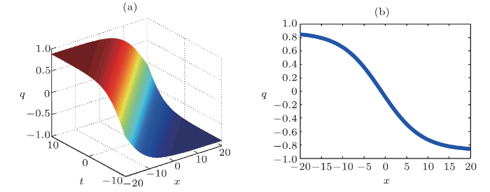
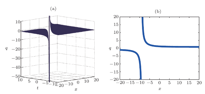
The main objective of this part is to give some graphical representations of the solutions found concerning the FLE. For that, the following values are used: $w=2.0,a_{1} =0.1,a_{2} =0.5$, and $B=0.3$. In the case of Figs. 1--4, the constant $C$ is equal to $0.9$ while in the case of Fig. 5, this constant has the value $9.0$. These figures are plotted in 2D and 3D.

Fig. 1

New window|Download| PPT slide
Fig. 1(Color online) Graphical representation of solution (20).

Fig. 2

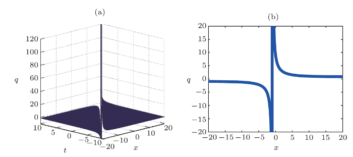New window|Download| PPT slide
Fig. 2(Color online) Graphical representation of solution (21).

Fig. 3

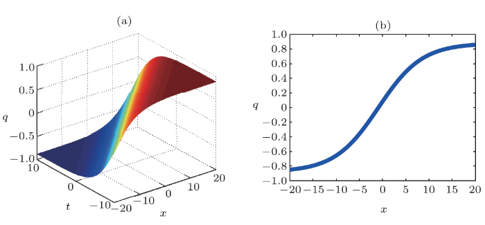New window|Download| PPT slide
Fig. 3(Color online) Graphical representation of solution (22).

Fig. 4

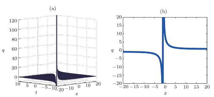New window|Download| PPT slide
Fig. 4(Color online) Graphical representation of solution (23) for $C = 0.9.$.

Fig. 5

New window|Download| PPT slide
Fig. 5(Color online) Graphical representation of solution (23) for $C = 9.0$.



The curves obtained are the amplitudes of the solutions and are solitary waves, particularly kink and anti-kink soliton solutions. These figures help to have a good idea on the dynamics of the perturbed Fokas-Lenells equation used in several domains such as the electronic communications Internet blogs, facebook communication as well as twitter comments. Thus, we notice that the FLE has a great importance in the nonlinear research. One of these interests also comes from the fact that the FLE contains rich physical features in solitary wave's theory and optical fibers phenomena. It is also important to mention that the outcomes of this work are new results not reported in the literature.

5 Conclusions

In this work, using the solution of the auxiliary equation (5) in the Riccati-Bernoulli Sub-ODE method, we have found some new exact solutions which are positives forward future studies for the perturbed Fokas-Lenells equation (FLE). Also the perturbation terms will be included to demonstrate the phenomena of soliton cooling, obtain quasi-monochromatic solitons, and establish quasi-particle theory to suppress intra-channel collision of optical solitons and several other features. In addition, stochastic perturbation terms will be included to analyze the corresponding Langevin equations in order to obtain mean free velocity of the soliton. We also conclude that this technique is a concise, effective, powerful, direct, and convenient method and can be applied to other nonlinear PDEs.

Reference View Option By original order
By published year
By cited within times
By Impact factor

[1] A. J. A. M. Jawad, A. Biswas, Q. Zhou , et al., Optik 165 ( 2018) 111.
[Cited within: 2]

[2] A. Bansal, A. H. Kara, A. Biswas , et al., Chaos, Solitons & Fractals 114 ( 2018) 275.
[Cited within: 1]

[3] A. Biswas, M. Ekici, A. Sonmezoglu, R. T. Alqahtani , Optik 165 ( 2018) 29.


[4] A. Biswas, Y. Yildirim, E. Yasar , et al., Optik 165 ( 2018) 74.


[5] A. Biswas, H. Rezazadeh, M. Mirzazadeh , et al., Optik 165 ( 2018) 288.
[Cited within: 1]

[6] A. Bekir , Phys. Lett. A 372 ( 2008) 3400.
[Cited within: 1]

[7] E. H. Zahran and M. M. Khater , American Journal of Computational Mathematics 4 ( 2014) 455.
[Cited within: 1]

[8] M. S. Shehata , International Journal of Computer Applications 109 ( 2015) 1.
[Cited within: 1]

[9] A. M. Wazwaz, Chaos, Solitons & Fractals 12 ( 2001) 1549.
[Cited within: 1]

[10] M. S. Shehata , International Journal of Physical Sciences 11 ( 2016) 80.
[Cited within: 2]

[11] X. F. Yang, Z. C. Deng, Y. Wei , Advances in Difference Equations 2015 ( 2015) 117.
[Cited within: 2]

[12] M. M. Khater, D. Lu, E. H. Zahran , Appl. Math. Inf. Sci. 11 ( 2017) 1.
[Cited within: 1]

[13] E. Tala-Tebue, Z. I. Djoufack, P. H. Kamdoum-Tamo, A. Kenfack-Jiotsa , Optik 174 ( 2018) 508.
[Cited within: 1]

[14] E. M. Zayed and H. Sayedahmed , International Journal of Computer Applications 67 ( 2013) 39.
[Cited within: 1]

[15] A. Biswas, M. O. Al-Amr, H. Rezazadeh , et al., Optik 165 ( 2018) 233.
[Cited within: 1]

[16] H. Rezazadeh, M. S. Osman, M. Eslami , et al., Optik 164 ( 2018) 84.
[Cited within: 1]

[17] M. S. Shehata , American Journal of Computational Mathematics 5 ( 2015) 468.
[Cited within: 1]

[18] E. H. Zahran , Journal of Computational and Theoretical Nanoscience 12 ( 2015) 5716.
[Cited within: 1]

[19] H. Rezazadeh , Optik 167 ( 2018) 218.
[Cited within: 1]

[20] H. Rezazadeh, H. Tariq, M. Eslami , et al., Chinese Journal of Physics 56 ( 2018) 2805.
[Cited within: 1]

[21] W. X. Ma and J. H. Lee, Chaos, Solitons and Fractals 42 ( 2009) 1356.
[Cited within: 1]

[22] W. X. Ma, J. Li, C.M. Khalique , Complexity 2018 ( 2018) 9059858.
[Cited within: 1]

[23] W. X. Ma , Front. Math. China 14 ( 2019) 619.
[Cited within: 1]

[24] W. X. Ma , East Asian Journal on Applied Mathematics 9 ( 2019) 185.


[25] W. X. Ma , J. Appl. Anal. Comput. 9 ( 2019) 1319.
[Cited within: 1]

[26] W. X. Ma and B. Fuchssteiner , Int. J. Non-Linear Mech. 31 ( 1996) 329.
[Cited within: 2]