Interaction Solutions for Kadomtsev-Petviashvili Equation with Variable Coefficients

删除或更新信息，请邮件至freekaoyan#163.com(#换成@)

本站小编 Free考研考试/2022-01-02

Jian-Guo Liu^,¹^,^?, Wen-Hui Zhu², Li Zhou¹1

College of Computer, Jiangxi University of Traditional Chinese Medicine, Jiangxi 330004, China;

Institute of Artificial Intelligence, Nanchang Institute of Science and Technology, Jiangxi 330108, China

Corresponding authors: ?E-mail:395625298@qq.com

Received:2019-03-18Online:2019-07-1

Fund supported:

^*Supported by National Natural Science Foundation of China under Grant.No. 81860771

Abstract
Based on the Hirota's bilinear form and symbolic computation, the Kadomtsev-Petviashvili equation with variable coefficients is investigated. The lump solutions and interaction solutions between lump solution and a pair of resonance stripe solitons are presented. Their dynamical behaviors are described by some three-dimensional plots and corresponding contour plots.
Keywords： Hirota's bilinear form;dynamical behaviors;stripe solitons

PDF (1159KB)Metadata Metrics Related articlesExportEndNote|Ris|Bibtex Favorite
Cite this article
Jian-Guo Liu, Wen-Hui Zhu, Li Zhou. Interaction Solutions for Kadomtsev-Petviashvili Equation with Variable Coefficients ^*. [J], 2019, 71(7): 793-797 doi:10.1088/0253-6102/71/7/793

1 Introduction

Nonlinear partial differential equations (NPDEs) are mathematical models to describe nonlinear phenomena in many fields of modern science and engineering, such as physical chemistry and biology, atmospheric space science, etc.^[1-6] In recent years, the solutions of NPDEs have become a hot topic, and various methods have been proposed.^[6-12]

In these NPDEs, Kadomtsev-Petviashvili (KP) equation can be used to model waves in ferromagnetic media, water waves of long wavelength with weakly non-linear restoring forces and frequency dispersion.^[13] However, when modeling various nonlinear phenomena under different physical backgrounds, variable coefficient NPDEs can describe the actual situation more accurately than constant coefficient NPDEs. As an illustration, a KP equation with variable coefficients is considered as follows^[14]

(1)$$ \alpha (t) u_x^2+\alpha (t) u u_{xx}+\beta (t) u_{xxxx}-\gamma (t) u_{yy}+u_{xt}=0\,, $$

where $u=u(x,y,t)$ is the amplitude of the long wave of two-dimensional fluid domain on varying topography or in turbulent flow over a sloping bottom. The B?cklund transformation, soliton solutions, Wronskian and Gramian solutions of Eq. (1) have been obtained.^[14-16] Lump and interactions solutions have been discussed in Ref. ^[17]. However, interactions among the lump soliton, one stripe soliton, and a pair of stripe solitons have not been investigated, which will become our main task.

The organization of this paper is as follows. Section 2 obtains the lump solutions based on Hirota's bilinear form and symbolic computation.^[18-34] Their dynamical behaviors are described in some plots. Section 3 derives the interaction solutions between lump solution and a pair of resonance stripe solitons. Their dynamical behaviors are also shown in some three-dimensional plots and corresponding contour plots. Section 4 makes a summary.

2 Lump Solutions

Substituting

$$\alpha(t)={6 \beta (t)}/{\Theta _0}\,, \ \ u=2\Theta _0[\ln\xi(x,y,t)]_{xx}$$

into Eq. (1), the bilinear form can be obtained as follows

(2)$$ [\beta(t) D_x^4-\gamma(t) D_y^2+ D_t D_x] \xi\cdot \xi=0\,. $$

This is equivalent to:

(3)$$ \xi [\beta (t) \xi_{xxxx}-\gamma (t) \xi_{yy}+\xi_{xt}]+3 \beta (t) \xi_{xx}^2 \\ \quad -4 \beta (t) \xi_x \xi_{xxx}+\gamma (t) \xi_y^2-\xi_t \xi_x=0\,. $$

To research the lump solutions, suppose that

(4)$$ \xi=\; [\Theta _3(t)+\Theta _1 x+\Theta _2 y]{}^2+[\Theta _6(t) \\ +\Theta _4 x+\Theta _5 y]{}^2+\Theta _7(t)\,, $$

where $\Theta _i\;(i=1,2,4,5)$ are unknown constants. $\Theta _3(t)$ and $\Theta _6(t)$ are unkown functions. Substituting Eq. (4) into Eq. (3), we have

(5)$$ \beta(t)=\zeta _1 \gamma (t)\,, \quad \Theta_7(t)=\frac{3 \zeta _1 (\Theta _1^2+\Theta _4^2)^3}{(\Theta _2 \Theta _4-\Theta _1 \Theta _5)^2}\,, \Theta_3(t)=\int_1^t \frac{(2 \Theta _2 \Theta _4 \Theta _5+\Theta _1 (\Theta _2^2-\Theta _5^2)) \gamma (t)}{\Theta _1^2+\Theta _4^2} d t+\tau _1\,, \Theta_6(t)=\int_1^t \frac{(-\Theta _4 \Theta _2^2+2 \Theta _1 \Theta _5 \Theta _2+\Theta _4 \Theta _5^2) \gamma (t)}{\Theta _1^2+\Theta _4^2} d t+\tau _2\,, $$

with $\Theta _1^2+\Theta _4^2 \neq 0$, $\Theta _2 \Theta _4-\Theta _1 \Theta _5 \neq 0$. $\tau _i\;(i=1,2)$ are integral constants. Substituting Eq. (5) into Eq. (4) and the transformation $u=2\Theta _0[\ln\xi]_{xx}$, the lump solutions for Eq. (1) can be presented as follows

(6)$$ u= \frac{2 \Theta _0 (\xi \xi_{xx}-\xi_x^2)}{\xi ^2}\,, $$

where $\xi$ satisfies constraint condition (5).

To discuss the dynamical behaviors for solution (6), we suppose that

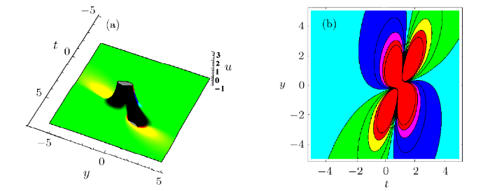
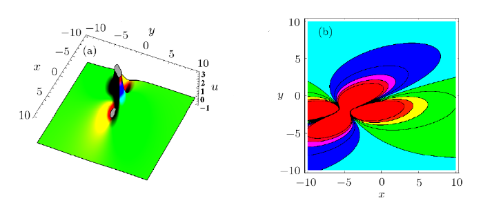
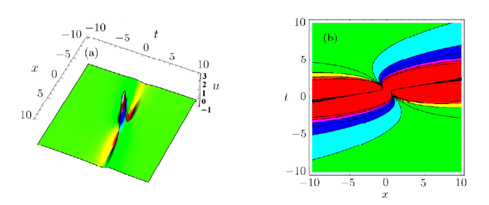
(7)$$ \Theta _1=\Theta_4=\Theta_5=-1\,, \quad \Theta_2=\Theta_0=3\,, \\ \zeta_1=\gamma(t)=1\,,\quad \tau_1=\tau_2=0\,. $$

Substituting Eq. (7) into Eq. (6), three-dimensional plots and corresponding contour plots are presented in Figs. 1--3, Figure 1 shows the spatial structure of the bright lump solution on the $(y,t)$ plane, which includes one peak and two valleys. Figure 2 shows the spatial structure of the bright lump solution on the $(y,x)$ plane. Figure 3 shows the spatial structure of the bright lump solution on the $(t,x)$ plane.

Fig. 1

New window|Download| PPT slide
Fig. 1(Color online) Lump solution (6) via Eq. (7) when $x= 0$ (a) three-dimensional graph (b) contour graph.

Fig. 2

New window|Download| PPT slide
Fig. 2(Color online) Lump solution (6) via Eq. (7) when $t= 0$ (a) three-dimensional graph (b) contour graph.

Fig. 3

New window|Download| PPT slide
Fig. 3(Color online) Lump solution (6) via Eq. (7) when $y= 0$ (a) three-dimensional graph (b) contour graph.

3 Interaction Solutions Between Lump Solution and a Pair of Resonance Stripe Solitons

To find the interaction solutions between the lump solution and a pair of resonance stripe solitons, assume that

(8)$$ \xi= [\Theta _3(t)+\Theta_1 x+\Theta _2 y]^2 +[\Theta _6(t)+\Theta _4 x+\Theta _5 y]^2+\Theta _7(t) +\sigma _1(t) e^{\zeta _3(t)+\zeta _1 x+\zeta _2 y}+\sigma _2(t) e^{-\zeta _3(t)-\zeta _1 x-\zeta _2 y}\,, $$

where $\vartheta _i\;(i=1,2,4,5)$ and $\zeta _i\;(i=1,2)$ are unknown constants. $\Theta _3(t)$, $\Theta _6(t)$, $\zeta _3(t)$, and $\sigma _i(t)\;(i=1,2)$ are unkown functions. Substituting Eq. (4) into Eq. (3), we have

(9)$$ \sigma _2(t)= \frac{\eta _1}{\sigma _1(t)}\,, \quad \Theta_7(t)=\frac{\zeta _1^4 \eta _1+(\Theta _1^2+\Theta _4^2)^2}{\zeta _1^2 (\Theta _1^2+\Theta _4^2)}\,, \quad \Theta_5=\frac{\zeta _2 (\Theta _1^2+\Theta _4^2)-\zeta _1 \Theta _1 \Theta _2}{\zeta _1 \Theta _4}\,, \\ \Theta_3(t)=\kappa _1-\int_1^t \frac{[\Theta _1 (\zeta _2 \Theta _1-\zeta _1 \Theta _2)^2+\zeta _2 \Theta _4^2 (\zeta _2 \Theta _1-2 \zeta _1 \Theta _2)] \gamma (t)}{\zeta _1^2 \Theta _4^2} d t\,, \\ \Theta_6(t)=\kappa _2+\int_1^t \frac{[\zeta _2^2 (\Theta _1^2+\Theta _4^2)-\zeta _1^2 \Theta _2^2] \gamma (t)}{\zeta _1^2 \Theta _4} d t\,, \quad \frac{\beta(t)}{ \gamma (t)}=\frac{(\zeta _2 \Theta _1-\zeta _1 \Theta _2)^2}{3 \zeta _1^4 \Theta _4^2}\,, \\ \zeta _3(t)=\kappa _3-\int_1^t \frac{[(\zeta _2 \Theta _1-\zeta _1 \Theta _2)^2-3 \zeta _2^2 \Theta _4^2] \gamma (t) \sigma _1(t)+3 \zeta _1 \Theta _4^2 \sigma _1'(t)}{3 \zeta _1 \Theta _4^2 \sigma _1(t)} d t\,, $$

with $\zeta _1^2 (\Theta _1^2+\Theta _4^2) \neq 0$, $\Theta _4 \neq 0$. $\eta _1$ and $\kappa _i\;(i=1,2,3)$ are integral constants. Substituting Eq. (9) into Eq. (8) and the transformation $u=2\Theta _0\,[\ln\xi]_{xx}$, the interaction solutions between lump solution and two stripe solitons can be presented as follows

(10)$$ u= \frac{2 \Theta _0 (\xi \xi_{xx}-\xi_x^2)}{\xi ^2}\,, $$

where $\xi$ satisfies constraint condition (9).

To discuss the dynamical behaviors for solution (10), we suppose that

(11)$$ \Theta _1=\Theta_4=-1\,, \ \ \Theta_2=\Theta_0=3\,, \ \ \zeta_1=\sigma _1(t)=1\,, \quad \zeta_2=2\,, \quad \kappa_1=\kappa_2=\kappa_3=0\,. $$

Substituting Eq. (11) into Eq. (10), three-dimensional plots and corresponding contour plots are presented in Figs. 4--8.

Fig. 4

New window|Download| PPT slide
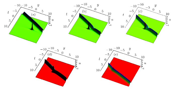
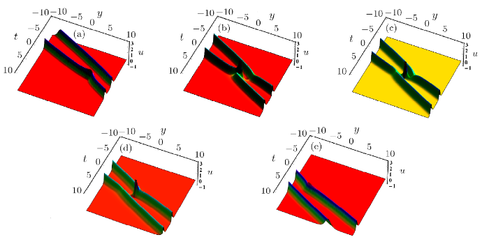
Fig. 4(Color online) Solution (10) via Eq. (11) with $\gamma(t)=1$,$\eta_1=0$ when (a) $x= -20$, (b) $x= -5$, (c) $x= 0$, (d) $x= 5$,(e) $x= 20$.

Fig. 5

New window|Download| PPT slide
Fig. 5(Color online) The corresponding contour plots of Fig. 4.

Fig. 6

New window|Download| PPT slide
Fig. 6(Color online) Solution (10) via Eq. (11) with $\gamma(t)=1$,$\eta_1=1$ when (a) $x= -20$, (b) $x= -5$, (c) $x= 0$, (d) $x= 5$,(e) $x= 20$.

Fig. 7

New window|Download| PPT slide
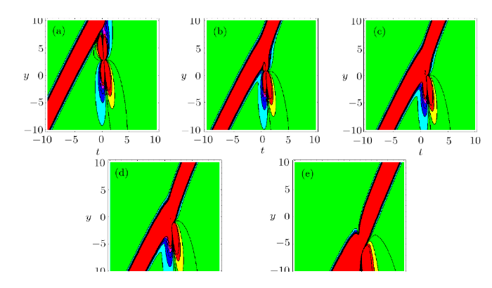
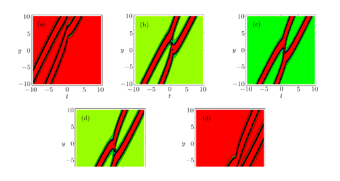
Fig. 7(Color online) The corresponding contour plots of Fig. 6.

Fig. 8

New window|Download| PPT slide
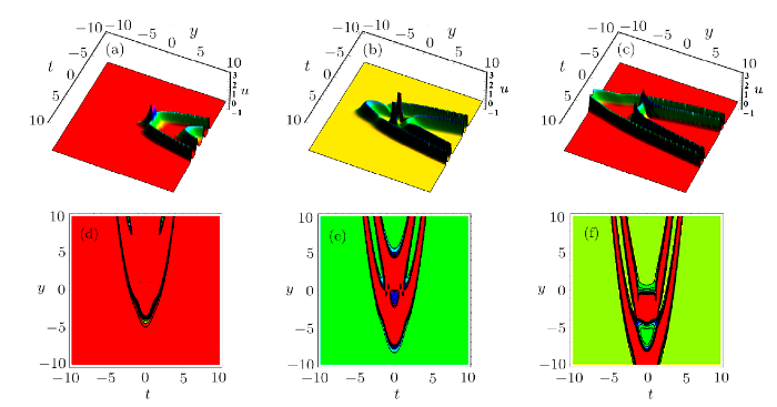
Fig. 8(Color online) Solution (10) via Eq. (11) with $\gamma(t)=t$,$\eta_1=1$ when $x= -10$ in (a) (d), $x= 0$ in (b) (e), and $x =10$ in (c) (f).

When $\eta_1=0$, Figs. 4 and 5 describe the interaction solution between lump solution and one stripe soliton in the $(t,y)$-plane, the fusion between the lump soliton and one stripe soliton is shown in Fig. 4. When $x=-20$, one lump and one stripe soliton can be found in Fig. 4(a). In Fig. 4(b), the lump soliton meets with one stripe soliton. In Figs. 4(c) and 4(d), we can see the interaction between the lump and one stripe soliton. In Fig. 4(e), lump starts to be swallowed until lump blend into one stripe soliton and go on spreading. Figure 5 shows the corresponding contour plots of Fig. 4.

When $\eta_1=1$, Figs. 6, 7, and 8 demonstrate the interaction solution between lump solution and a pair of resonance stripe soliton in the $(t,y)$-plane, the fusion between the lump soliton and two stripe solitons is shown in Fig. 6. When $x=-20$, two stripe solitons and one lump can be found in Fig. 6(a). In Fig. 6(b), the lump soliton meets with two stripe soliton. In Figs. 6(c) and 6(d), we can see the interaction between the lump and two stripe solitons. In Fig. 6(e), lump starts to be swallowed until lump blend into two stripe solitons and go on spreading. Figure 7 shows the corresponding contour plots of Fig. 6 to help us better understand the interaction for solution (10). Figure 8 lists the interaction between the lump and two stripe solitons when $\gamma(t)=t$ is a function.

4 Conclusion

In this work, the (2+1)-dimensional KP equation with variable coefficients are studied based on Hirota's bilinear form and symbolic computation. Lump solutions and interaction solutions are presented. The spatial structure of the bright lump solution are shown in Figs. 1--3. The dynamical behaviors for the interaction solutions between lump solution and one stripe soliton are described in Figs. 4 and 5. The dynamical behaviors for the interaction solutions between lump solution and a pair of resonance stripe solitons are shown in Figs. 6--8.

The authors have declared that no competing interests exist.

Reference By original order
By published year
By cited within times
By Impact factor

[1]

J. J.

and Y. T.

Gao

, Superlattice. Microst. 104 ( 2017)498.

[Cited within: 1]

[2]

M. D.

Chen

, X.

, Y.

Wang

, B.

, Commun. Theor. Phys. 67 ( 2017)595.

[3]

W. X.

, Z. Y.

Qin

, X.

Lü

, Nonlinear Dyn. 84 ( 2016)923.

[4]

Z. Z.

Lan

and B.

Gao

, Appl. Math. Lett. 79 ( 2018)6.

[5]

Zhang

and Y.

Chen

, Nonlinear Dyn. 93 ( 2018)2169.

[6]

Z. Z.

Lan

and B.

Gao

, Eur. Phys. J. Plus. 132 ( 2017)512.

[Cited within: 2]

[7]

Zhang

, Z.

Han

, Y.

Chen

, Commun. Theor. Phys. 69 ( 2018)14.

[8]

M. S.

Osman

, J. A. T.

Machado

, D.

Baleanu

, Opt. Quant. Electron. 50 ( 2018)1.

[9]

L. L.

Huang

and Y.

Chen

, Nonlinear Dyn. 92 ( 2018)221.

[10]

X. Y.

Xie

and G. Q.

Meng

, Nonlinear Dyn. 93 ( 2018)779.

[11]

Qawasmeh

and M.

Alquran

, Appl. Math. Sci. 8 ( 2014)5985.

[12]

Eslami

and H.

Rezazadeh

, Calcolo. 53 ( 2016)1.

[Cited within: 1]

[13]

A. M.

Wazwaz

, Wave. Random. Complex. 29 ( 2019)195.

[Cited within: 1]

[14]

J. P.

, Chin. Phys. Lett. 28 ( 2011)060207.

[Cited within: 2]

[15]

Y. Y.

Wang

and J. F.

Zhang

, Phys. Lett. A 352 ( 2006)155.

[16]

Z. Z.

Yao

, C. Y.

Zhang

, et al., Commun. Theor. Phys. 49 ( 2008)1125.

[Cited within: 1]

[17]

X. Y.

Jia

, B.

Tian

, Z.

, et al., Mod. Phys. Lett. B 32 ( 2018)1850086.

[Cited within: 1]

[18]

W. X.

, J. Geom. Phys. 132 ( 2018)45.

[Cited within: 1]

[19]

A. M.

Wazwaz

and S. A.

El-Tantawy

, Nonlinear Dyn. 87 ( 2017)2457.

[20]

X. Y.

Xie

and G. Q.

Meng

, Appl. Math. Lett. 92 ( 2019)201.

[21]

A. M.

Wazwaz

, Nonlinear Dyn. 91 ( 2018)877.

[22]

W. X.

, X. L.

Yong

, H. Q.

Zhang

, Comput. Math. Appl. 75 ( 2018)289.

[23]

Eslami

, B. F.

Vajargah

, M.

Mirzazadeh

, A.

Biswas

, Indian J. Phys. 88 ( 2014)177.

[24]

A. M.

Wazwaz

and S. A.

El-Tantawy

, Nonlinear Dyn. 84 ( 2016)1107.

[25]

W. X.

and Y.

Zhou

, J. Differ. Equations 264 ( 2018)2633.

[26]

$\dot{\rm I}$smail

, Math. Meth. Appl. Sci. 34 ( 2011)990.

[27]

Alquran

, H. M.

Jaradat

, M. I.

Syam

, Nonlinear Dyn. 90 ( 2017)2525.

[28]

L. L.

Huan

and Y.

Chen

, Commun. Nonlinear Sci. Numer. Simulat. 67 ( 2019)237.

[29]

A. M.

Wazwaz

, Nonlinear Dyn. 93 ( 2018)1371.

[30]

S. T.

Chen

and W. X.

, Comput. Math. Appl. 76 ( 2018)1680.

[31]

S. T.

Chen

and W. X.

, Front. Math. China 13 ( 2018)525.

[32]

W. X.

, J. Geom. Phys. 133 ( 2018)10.

[33]

Y. F.

Yue

, L. L.

Huang

, Y.

Chen

, Appl. Math. Lett. 89 ( 2019)70.

[34]

L. L.

Huang

, Y. F.

Yue

, Y.

Chen

, Comput. Math. Appl. 76 ( 2018)831.

[Cited within: 1]

闂傚倷绀佺紞濠傖缚瑜旈、鏍幢濡炵粯鏁犻梺閫炲苯澧撮柣鎿冨亰瀹曞墎鎹勬潪鏉挎瀳闂備線鈧偛鑻晶浼存煕閻樻煡鍙勭€规洏鍨芥俊鍫曞炊閵娿儺浼曢梺鑽ゅ枑閻熴儳鈧凹鍙冨鎶藉醇閵夛妇鍘遍梺褰掑亰閸撴瑩銆冨▎鎴犵＜闁告瑦锚瀹撳棛鈧娲忛崝鎴﹀极閹剧粯鏅搁柨鐕傛嫹闂傚倷鐒︾€笛呯矙閹达附鍎斿┑鍌氭啞閸嬬喐绻涢幋娆忕仼缁绢厸鍋撻梺璇查濠€杈ㄦ叏鐎靛摜涓嶆い鏍仦閻撴洘绻涢崱妯哄濠⒀屽墯缁绘繈鍩€椤掑嫬绠ユい鏃€鍎冲畷銉モ攽閻愬弶顥為悽顖滃仱婵″爼顢曢敂鐣屽幐闂佺ǹ鏈粙鎾诲箠閸℃瑦鍋栨繛鍡樻尰閻撴洘淇婇娆掝劅闁稿孩鍨圭槐鎾诲磼濮樺吋楔闂侀€炲苯澧存繛浣冲吘娑樷槈閵忊€充函濠电姴锕ら悧濠囧疾椤掑嫭鐓ラ柣鏇炲€圭€氾拷