Tao Fang¹, Hui Wang^,1,2,??, Yun-Hu Wang^1,3, Wen-Xiu Ma^{2,4,5,6 1} College of Art and Sciences, Shanghai Maritime University, Shanghai 201306, China
² Department of Mathematics and Statistics, University of South Florida, Tampa, FL 33620, USA
³ Department of Mathematics and Information Technology, The Education University of Hong Kong, Hong Kong, China
⁴ Department of Mathematics, King Abdulaziz University, Jeddah, Saudi Arabia
⁵ College of Mathematics and System Science, Shandong University of Science and Technology, Qingdao 266590, China
⁶ Department of Mathematical Sciences, North-West University, Mafikeng Campus, Mmabatho 2735, South Africa

Corresponding authors: ? E-mailhwang@shmtu. edu. cn

Received:2018-12-31Online:2019-08-1

Fund supported:

* Supported by the National Natural Science Foundation of China under Grant .Nos. 11571008 the National Natural Science Foundation of China under Grant.Nos. 51679132 National Science Foundation under Grant.No. DMS-1664561 and the Shanghai Science and Technology Committee under Grant .No. 17040501600

Abstract
By means of the Hirota bilinear method and symbolic computation, high-order lump-type solutions and a kind of interaction solutions are presented for a (3+1)-dimensional nonlinear evolution equation. The high-order lump-type solutions of the associated Hirota bilinear equation are presented, which is a kind of positive quartic-quadratic-function solution. At the same time, the interaction solutions can also be obtained, which are linear combination solutions of quartic-quadratic-functions and hyperbolic cosine functions. Physical properties and dynamical structures of two classes of the presented solutions are demonstrated in detail by their graphs.
Keywords： high-order lump-type solutions;interaction solutions;Hirota bilinear method


PDF (19427KB)MetadataMetricsRelated articlesExportEndNote|Ris|BibtexFavorite
Cite this article
Tao Fang, Hui Wang, Yun-Hu Wang, Wen-Xiu Ma. High-Order Lump-Type Solutions and Their Interaction Solutions to a (3+1)-Dimensional Nonlinear Evolution Equation ^*. [J], 2019, 71(8): 927-934 doi:10.1088/0253-6102/71/8/927

1 Introduction

The investigation of rational solutions on nonlinear evolution equations (NLEEs) has attracted much attention from mathematicians, physicists, and many scientists in other fields. Among these rational solutions,^[1] lump solutions and rogue wave solutions have been found in many integrable systems. ^[2-7] Recently, the study of lump solutions, which rationally localized in all directions in the space, becomes a hot topic in soliton theory. ^[8-22] Over the past decades, many powerful methods have been developed to find the lump solutions of NLEEs, such as the Hirota bilinear method,^[23] the long wave limit approach,^[3] and the nonlinear superposition formulae. ^[24] Among these methods, the Hirota bilinear method is a direct method, which can be used to obtain the exact solutions for NLEEs once its corresponding bilinear form is given. By taking the function $f$ in the bilinear equation as a positive quadratic function, Ref. [8] obtained the lump solutions of the KPI equation, which can be reduced to the ones in Refs. [3,25]. Then, this method is widely used to find lump solutions or lump-type solutions for generalized fifth-order KdV equation, Boussinesq equation, (4+1)-dimensional Fokas equation and so on. ^[11-21] References [26-44] further extended this method to find interaction solutions for integrable and non-integrable system.

In this paper, we focus on the following (3+1)-dimensional NLEE

(1) $$3u_{xz}-(2u_t+u_{xxx}-2uu_x)_y+2(u_x\partial_x^{-1}u_y)_x=0\,, $$
where the inverse operator $\partial_x^{-1}$ is defined as $(\partial_x^{-1} f )(x) = \int_{-\infty}^{x} f(x'){\rm d}x'$ under the decaying condition at infinity and $\partial_x = \partial / \partial_x$ with the condition

$\partial_x\partial_x^{-1} = \partial_x^{-1}\partial_x = 1$. This equation was first introduced in Ref. [45] studied the algebraic-geometrical solutions. Based on the constructed Wronskian determinant of solutions for a system of four linear differential equations, $N$-soliton solution and its Wronskian form are given in Ref. [46]. The linear superposition principle of Eq. (1) has also discussed in Ref. [47]. The Darboux transformation and the solutions of multiple soliton interactions were studied in Ref. [48]. Positon, negaton, soliton and their interaction solutions, multiple soliton solutions and multiple singular soliton solutions are explicitly obtained by using the Hirota's direct method in Refs. [49-50]. Reference [7] constructed its rouge waves and rational solutions by a simple symbolic computation approach. Recently, $M$-lump solutions of Eq. (1) and the interaction solutions between stripe solitons and lumps are discussed in Ref. [19]. To the best of our knowledge, the high-order lump-type solutions by taking the function $f$ in the bilinear equation as a kind of positive quartic-quadratic-functions, and the interaction solutions by taking the function $f$ as a combination of the positive quartic-quadratic-functions and hyperbolic cosine functions have not been studied so far. The aim of this paper is to discuss the high-order lump-type solutions and the interaction solutions to the (3+1)-dimensional NLEE (1). Through the dependent variable transformation

(2) $$u = -3[\,\ln f(x,y,z,t)]_{xx}\,, $$
Eq. (1) is transformed into the Hirota bilinear form

(3) $$(D_yD_x^3-3D_xD_z+2D_yD_t)f\cdot f=0\,, $$
where the derivatives $D_yD_x^3$, $D_xD_z$, and $D_yD_t$ are the bilinear operators defined by^[23]

(4) $$D^{n_1}_{x_1}\cdots D^{n_l}_{x_l}F \cdot G\!=\!(\partial_{x_1}\!-\partial_{x'_1})^{n_1}\!\cdots(\partial_{x_l} -\partial_{x'_l})^{n_l}F(x_1,\ldots,x_l) \\ \quad \times \,G(x'_1,\ldots,x'_l)|_{x'_1=x_1,\ldots,x'_l=x_l}\,, $$
and the corresponding bilinear form of Eq. (3) equals to

(5) $$6(f_{xz}f\!-\!f_xf_z)-2(f_{xxxy}f\!-\!f_{xxx}f_y)+6(f_{xxy}f_x-6f_{xx}f_{xy}) \\ \quad -\,4(f_{yt}f-4f_{y}f_t)=0\,. $$
The structure of this paper is as follows. In Sec. 2, high-order lump-type solutions are constructed by using the Hirota bilinear method, which are obtained by taking function $f$ in Eq. (3) as a kind of positive quartic-quadratic-functions. In Sec. 3, a kind of interaction solutions are derived by assuming function $f$ in Eq. (3) as a combination of positive quartic-quadratic-functions and hyperbolic cosine functions. Finally, some conclusions will be given in Sec. 4.

2 High-Order Lump-Type Solutions for

Eq. (1)

In this section, we will construct high-order lump-type solutions of Eq. (1) by taking $f$ in Eq. (3) as a combination of positive quartic-quadratic-functions

(6) $$f=s^4+g^2+h^2+a_{16}\,, $$
with

(7) $$s=a_1x+a_2y+a_3z+a_4t+a_5\,,\\ g=a_6x+a_7y+a_8z+a_9t+a_{10}\,,\\ h=a_{11}x+a_{12}y+a_{13}z+a_{14}t+a_{15}\,, $$
where the real parameters $a_i (1\leq i \leq 16) $ will be determined later. Substituting ansatz (6) with (7) into Eq. (3) with a direct symbolic computation, it generates the following results

(8) $$a_1=a_4=0\,,\quad a_7=-\frac{a_{11}a_{12}}{a_6}\,,\quad a_8=-\frac{a_3a_{11}a_{12}}{a_2a_6}\,,\\ a_9=\frac{3a_3a_6}{2a_2}\,,\quad a_{13}=\frac{a_3a_{12}}{a_2}\,,\quad a_{14}=\frac{3a_3a_{11}}{2a_2}\,,\\ a_{15}=\frac{a_2a_6a_{10}a_{11}+a_5a_{11}^2a_{12}+a_5a_6^2a_{12}}{a_2a_6^2}\,, $$
which need to satisfy constraint conditions as follows

(9) $$a_2a_6\neq 0\,, \quad a_{16} > 0\,, $$
to ensure the corresponding solution $f$ is well defined. With the constraint conditions (9) and transformation (2), the solution (6) can be obtained as follows

(10) $$u=\frac{12(a_6g+a_{11}h)^2}{f^2}-\frac{6(a_6^2+a_{11}^2)}{f}\,, $$
where

(11) $$f=(a_2y+a_3z+a_5)^4+g^2+h^2+a_{16}\,,\\ g=a_6x-\frac{a_{11}a_{12}}{a_6}y-\frac{a_3a_{11}a_{12}}{a_2a_6}z+\frac{3a_3a_6}{2a_2}t+a_{10}\,,\\ h=a_{11}x+a_{12}y+\frac{a_3a_{12}}{a_2}z+\frac{3a_3a_{11}}{2a_2}t\\ \quad \;\, +\frac{a_2a_6a_{10}a_{11} +a_5a_{11}^2a_{12}+a_5a_6^2a_{12}}{a_2a_6^2}\,. $$
Case 1 By taking $y=0$, the solution (10) can be reduced to the following form

(12) $$u=\frac{12(a_6g+a_{11}h)^2}{f^2}-\frac{6(a_6^2+a_{11}^2)}{f}\,, $$
with

(13) $$2 f=(a_3z+a_5)^4+g^2+h^2+a_{16}\,,\\ g=a_6x-\frac{a_3a_{11}a_{12}}{a_2a_6}z+\frac{3a_3a_6}{2a_2}t+a_{10}\,,\\ h=a_{11}x+\frac{a_3a_{12}}{a_2}z+\frac{3a_3a_{11}}{2a_2}t\\ \quad\;\; +\frac{a_2a_6a_{10}a_{11} +a_5a_{11}^2a_{12}+a_5a_6^2a_{12}}{a_2a_6^2}\,. $$
It is easy to calculate that there are three critical points to solution (12), which reads

(14) $$(x_{u_1},z_{u_1})=\Bigl(-\frac{3a_{3}a_{6}^{2}t+2a_{10}a_{2}a_{6}+2a_{11}a_{12}a_{5}}{2a_{6}^{2}a_{2}}, -\frac{a_{5}}{a_{3}}\Bigr),\\ (x_{u_2},z_{u_2})=\Bigl(\frac{-3a_{11}^{2}a_{3}a_{6}^{2}t-3a_{3}a_{6}^{4}t-2a_{10}a_{11}^{2}a_{2}a_{6} -2a_{10}a_{2}a_{6}^{3}-2a_{11}^{3}a_{12}a_{5}-2a_{12}a_{11}a_{5}a_{6}^{2}}{2a_{6}^{2}a_{2}(a_{11}^{2} +a_{6}^{2})}\\ \quad\quad\quad\quad\quad+\frac{2\sqrt{3a_{11}^{2}a_{16}a_{2}^{2}a_{6}^{4}+3a_{16}a_{2}^{2}a_{6}^{6}}}{2a_{6}^{2}a_{2}(a_{11}^{2}+a_{6}^{2})}, -\frac{a_{5}}{a_{3}}\Bigr),\\ (x_{u_3},z_{u_3})=\Bigl(\frac{-3a_{11}^{2}a_{3}a_{6}^{2}t-3a_{3}a_{6}^{4}t-2a_{10}a_{11}^{2}a_{2}a_{6} -2a_{10}a_{2}a_{6}^{3}-2a_{11}^{3}a_{12}a_{5}-2a_{12}a_{11}a_{5}a_{6}^{2}}{2a_{6}^{2}a_{2}(a_{11}^{2} +a_{6}^{2})}\\ \quad\quad\quad\quad\quad-\frac{2\sqrt{3a_{11}^{2}a_{16}a_{2}^{2}a_{6}^{4}+3a_{16}a_{2}^{2}a_{6}^{6}}}{2a_{6}^{2}a_{2} (a_{11}^{2}+a_{6}^{2})},-\frac{a_{5}}{a_{3}}\Bigr). $$
In order to show the physical properties and structures of solutions (12) more clearly, we select the parameters as

$a_2=1,a_3=0. 2,a_5=0,a_6=1,a_{10}=1,a_{11}=1,a_{12}=5,a_{16}=1$, which yields

(15) $$u=\frac{24(-16z^2\!+\!9. 6xt\!+\!1. 44t^2\!-\!0. 0128z^4\!+\!16x^2\!-\!8)}{(0. 72t^2\!+\!8x^2\!+\!8z^2\! +\!4. 8xt\!+\!0. 0064z^4\!+\!4)^2}, $$
and the corresponding three critical points can be further calculated as follows

(16a)$$(x_{u_1},z_{u_1})=(-0. 3t,0)\,,$$
(16b)$$(x_{u_2},z_{u_2})=\Bigl(-0. 3t+\frac{\sqrt{6}}{2},0\Bigr),$$
(16c)$$(x_{u_3},z_{u_3})=\Bigl(-0. 3t-\frac{\sqrt{6}}{2},0\Bigr). $$
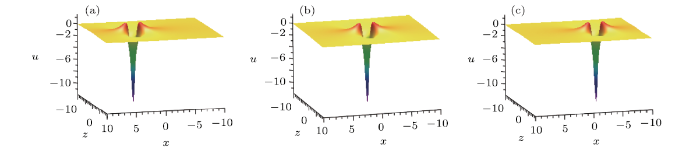
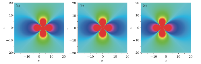
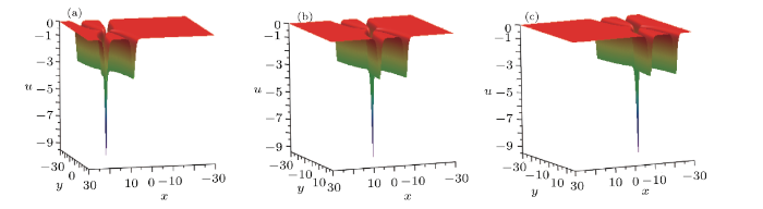
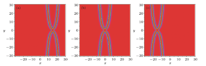
It is easy to found that solution (15) has a local minimum value $u_{\rm min} = -12$ at $(-0. 3t, 0)$ and a local maximum value $u_{\rm max} = 1. 5$ at $(-0. 3t+({\sqrt{6}}/{2}),0)$ and $(-0. 3t-({\sqrt{6}}/{2}),0)$, which can be clearly observed from Fig. 1. Figure 2 is the corresponding density-plots in the $(x, z)$-plane when $t =-10, 0, 10$, respectively.

Fig. 1

New window|Download| PPT slide
Fig. 1(Color online) Evolution plots of the solution (15). (a) $t=-10$, (b) $t=0$, (c) $t=10$.

Fig. 2

New window|Download| PPT slide
Fig. 2(Color online) Corresponding density plots for Fig. 1. (a) $t=-10$, (b) $t=0$, (c) $t=10$.



it Case 2 By taking $z=0$, the solution (10) can be reduced to the following form

(17) $$u=\frac{12(a_6g+a_{11}h)^2}{f^2}-\frac{6(a_6^2+a_{11}^2)}{f}\,,$$
where

(18) $$f=(a_2y+a_5)^4+g^2+h^2+a_{16}\,,\quad g=a_6x-\frac{a_{11}a_{12}}{a_6}y+\frac{3a_3a_6}{2a_2}t+a_{10}\,,\\ h=a_{11}x+a_{12}y+\frac{3a_3a_{11}}{2a_2}t+\frac{a_2a_6a_{10}a_{11}+a_5a_{11}^2a_{12} +a_5a_6^2a_{12}}{a_2a_6^2}\,. $$
It is easy to find that solution (17) also has three critical points

(19) $$(x_{u_1},y_{u_1})=\Bigl(-\frac{3a_{3}a_{6}^{2}t+2a_{10}a_{2}a_{6}+2a_{11}a_{12}a_{5}}{2a_{6}^{2}a_{2}}, -\frac{a_{5}}{a_{2}}\Bigr),\\ (x_{u_2},y_{u_2})=\Bigl(\frac{-3a_{11}^{2}a_{3}a_{6}^{2}t-3a_{3}a_{6}^{4}t-2a_{10}a_{11}^{2}a_{2} a_{6}-2a_{10}a_{2}a_{6}^{3}-2a_{11}^{3}a_{12} a_{5}-2a_{12}a_{11}a_{5}a_{6}^{2}}{2a_{6}^{2}a_{2}(a_{11}^{2}+a_{6}^{2})}\\ \quad\quad\quad\quad\quad+\frac{2\sqrt{3a_{11}^{2}a_{16}a_{2}^{2}a_{6}^{4}+3a_{16}a_{2}^{2}a_{6}^{6}}}{2a_{6}^{2}a_{2} (a_{11}^{2}+a_{6}^{2})},-\frac{a_{5}}{a_{2}}\Bigr),\\ (x_{u_3},y_{u_3})=\Bigl(\frac{-3a_{11}^{2}a_{3}a_{6}^{2}t-3a_{3}a_{6}^{4}t-2a_{10}a_{11}^{2} a_{2}a_{6}-2a_{10}a_{2}a_{6}^{3}-2a_{11}^{3}a_{12}a_{5}-2a_{12}a_{11}a_{5} a_{6}^{2}}{2a_{6}^{2}a_{2}(a_{11}^{2}+a_{6}^{2})}\\ \quad\quad\quad\quad\quad-\frac{2\sqrt{3a_{11}^{2}a_{16}a_{2}^{2}a_{6}^{4}+3a_{16}a_{2}^{2}a_{6}^{6}}}{2a_{6}^{2}a_{2} (a_{11}^{2}+a_{6}^{2})}, -\frac{a_{5}}{a_{2}}\Bigr). $$
By taking the corresponding parameters as $a_2=1,a_3=0. 2,a_5=0,a_6=1,a_{10}=1,a_{11}=1,a_{12}=5,a_{16}=1$, solution (17) with (18) can be reduced to the following form

(20) $$u=\frac{384(-80y^4+225t^2+600xt+400x^2-100y^2-80)}{(16y^4+45t^2+120xt+80x^2+20y^2+16) (180t^2+320x^2+80y^2+480xt+64y^4+64)}\,,$$
and the corresponding three critical points reads

(21c)$$ (x_{u_1},y_{u_1})=(-0. 75t,0),$$
(21b)$$(x_{u_2},y_{u_2})=\Big(-0. 75t+\frac{\sqrt{15}}{5},0\Big),$$
(21c)$$(x_{u_3},y_{u_3})=\Big(-0. 75t-\frac{\sqrt{15}}{5},0\Big), $$
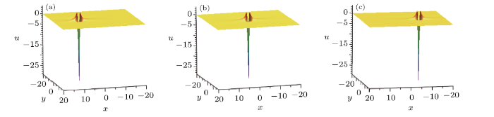
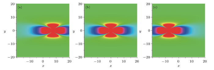
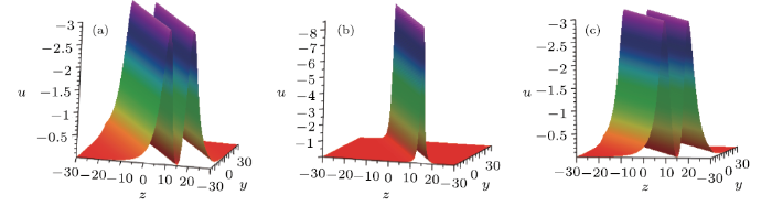
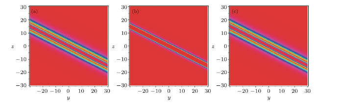
which point $(-0. 75t,0)$ corresponds to a local minimum value $u_{\rm min} = -30$, and points $(-0. 75t\pm ({\sqrt{15}}/{5}),0)$ correspond to a local maximum value $u_{\rm max} = 3. 75$.

For the corresponding $3$D-plots and density-plots, see Figs. 3 and 4.

Fig. 3

New window|Download| PPT slide
Fig. 3(Color online) Evolution plots of the solution (20). (a) $t=-10$, (b) $t=0$, (c) $t=10$.

Fig. 4

New window|Download| PPT slide
Fig. 4(Color online) Corresponding density plots for Fig. 3. (a) $t=-10$, (b) $t=0$, (c) $t=10$.



Case 3 When $x = 0$ and $a_5=0$, one can see that $g$ and $h$ in Eq. (11) satisfy, which means expression (6) can be rewritten as $f=s^4+(1+\alpha^2)h^2+a_{16}$. $g = -({a_{11}}/{a_6})h$ Unfortunately, $f=s^4+(1+\alpha^2)h^2+a_{16}$ will lead to solution $u$ is not localized in all directions in space. ^[13,41]

By choosing appropriate parameters with $a_2=2$, $a_3=1$, $a_5=0$, $a_6=2$, $a_{10}=0$, $a_{11}=1$, $a_{12}=1$, $a_{16}=1$, $x=0$, one can simplify solution (10) to the following form

(22) $$u=\frac{480(-256y^4-512y^3Z-384y^2z^2-128yz^3-16z^4+45t^2-20y^2-20yz-5z^2-16)} {(256y^4+512y^3Z+384y^2z^2+128yz^3+16z^4+45t^2+20y^2+20yz+5z^2+16)^2}\,,$$
which corresponding $3$D-plots and density-plots can be seen in Figs. 5 and 6.

Fig. 5

New window|Download| PPT slide
Fig. 5(Color online) Evolution plots of the solution (22). (a) $t=-10$, (b) $t=0$, (c) $t=10$.

Fig. 6

New window|Download| PPT slide
Fig. 6(Color online) Corresponding density plots for Fig. 5. (a) $t=-10$, (b) $t=0$, (c) $t=10$.

3 A Kind of Interaction Solutions for Eq. (1)

In order to find the interaction solutions to Eq. (1), the function $f$ in Eq. (3) may be taken as the following form

(23) $$f=s^4+g^2+h^2+q+a_{16},$$
with

(24) $$s=a_1x+a_2y+a_3z+a_4t+a_5\,,\\ g=a_6x+a_7y+a_8z+a_9t+a_{10}\,,\\ h=a_{11}x+a_{12}y+a_{13}z+a_{14}t+a_{15}\,,\\ q=k\cosh(k_1x+k_2y+k_3z+k_4t)\,,$$
where the real parameters $a_i (1\leq i \leq 16) $ and $ k, k_j (1\leq j\leq 4) $ are all to be determined later.

Substituting ansatz (23) with (24) into Eq. (3), we obtain

(25) $$a_1=a_4=a_5=a_6=a_9=a_{11}=a_{14}=k_2=k_3=0\,, \\ a_7=\frac{a_2a_8}{a_3}\,,\quad a_{12}=\frac{a_2a_{13}}{a_3}\,,\quad k_4=-\frac{k_1(a_2k_1^2-3a_3)}{2a_2}\,, $$
which need to satisfy the following constraint conditions

(26) $$a_2a_3\neq 0\,,\quad a_{16} > 0\,,\quad k > 0\,,$$
to ensure the corresponding solution $u$ is positive, analytical and localized in all directions in the ($x,y,z$)-plane. With the conditions (25) and (26), the solution of Eq. (1) can be obtained as follows

(27) $$u=-\frac{3kk_1^2(s^4+g^2+h^2)\cosh(\xi)+3k^2k_1^2}{[s^4+g^2+h^2+k\cosh(\xi)]^2}\,, $$
with

(28) $$s = a_2y+a_3z\,,\quad g = \frac{a_2a_8}{a_3}y+a_8z+a_{10}\,,\quad h = \frac{a_2a_{13}}{a_3}y+a_{13}z+a_{15}\,,\quad \xi = k_1x-\frac{k_1(a_2k_1^2-3a_3)}{2a_2}t\,. $$
Case 1 Taking $a_2=0. 5,a_3=2,a_8=1,a_{10}=0,a_{13}=1,a_{15}=0,a_{16}=2,k=5,k_{1}=2,y=0$, solution (27) can be reduced to the following form

(29) $$u=-\frac{960(16\cosh(8t+2x)z^4+2\cosh(8t+2x)z^2+2\cosh(8t+2x)+5)} {(64z^4+8z^2+20\cosh(8t+2x)+8)^2}\,,$$
which corresponding $3$D-plots and density-plots can be seen in Figs. 7 and 8.

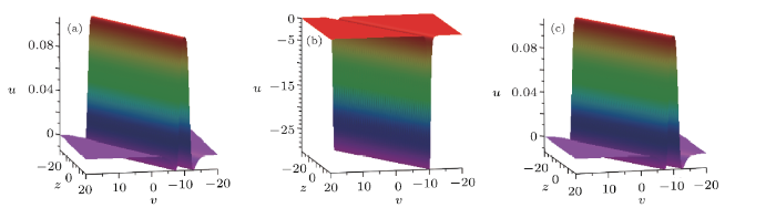
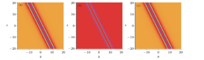
Case 2 By selecting the parameters as $a_2=1,a_3=2,a_8=4,a_{10}=0,a_{13}=2,a_{15}=0,a_{16}=1,k=4,k_{1}=2,z=0$, solution (27) can be rewritten as

(30) $$u=-\frac{48(\cosh(2t+2x)y^4+5\cosh(2t+2x)y^2+\cosh(2t+2x)+4)} {(y^4+5y^2+4\cosh(2t+2x)+1)^2}\,,$$
which corresponding $3$D-plots and density-plots can be seen in Figs. 9 and 10. From Figs. 7, 8, 9, and 10, it can be clearly seen that the above two types of solutions (29) and (30) can be regarded as "soliton" solutions.

Fig. 7

New window|Download| PPT slide
Fig. 7(Color online) Evolution plots of the solution (27). (a) $t=-5$, (b) $t=0$, (c) $t=5$.

Fig. 8

New window|Download| PPT slide
Fig. 8(Color online) Corresponding density plot for Fig. 7. (a) $t=-5$, (b) $t=0$, (c) $t=5$.

Fig. 9

New window|Download| PPT slide
Fig. 9(Color online) Evolution plots of the solution (30). (a) $t=-15$, (b) $t=0$, (c) $t=15$.

Fig. 10

New window|Download| PPT slide
Fig. 10(Color online) Corresponding density plot for Fig. 9. (a) $t=-15$, (b) $t=0$, (c) $t=15$.



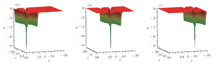
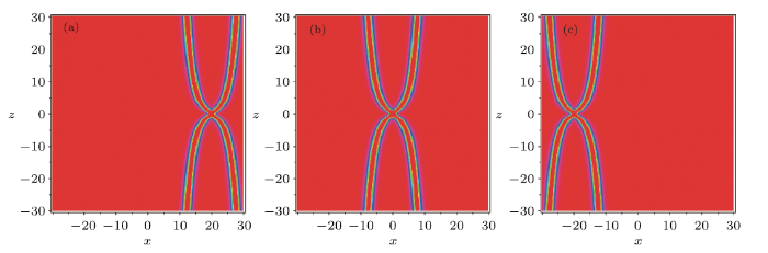
Case 3 By choosing appropriate parameters with $a_2=0. 5,a_3=1,a_8=2,a_{10}=0,a_{13}=2,a_{15}=0,a_{16}=2,k=5,k_{1}=2,x=0$, solution (27) reads

(31) $$u=\frac{-60(0. 0625y^4+0. 5y^3z+1. 5y^2z^2+2yz^3+z^4+2y^2+8yz+8z^2)\cosh(2t)-300} {(0. 0625y^4+0. 5y^3z+1. 5y^2z^2+2yz^3+z^4+2y^2+8yz+8z^2+5\cosh(2t)+2)^2}. $$
Figures 11 and 12 show the interaction phenomenon, which is induced by the twin-strip solitons for solution (31). Figures 11(a) and 12(a) show there are two stripe solitions at the time $t=-3$, and when $t=0$, the two stripes solitons disappear and one stripe soliton appears which has much more energy and higher peak that one can see in Figs. 11(b) and 12(b), as time goes by, the twin-strip solitons start appearing which can be seen in Figs. 11(c) and 12(c). In fact, in expression (28), $h=\beta g$ when $a_{13}=\beta a_8$, $a_{15}=\beta a_{10}$, which means the function $f$ in Eq. (23) could be rewritten as $f=s^4+(1+\beta^2)g^2+\cosh(\gamma t)$ under $x=0$. From Sec. 2, the function $f=s^4+(1+\beta^2)g^2$ yields lump-type solution along the direction of $x=0$. It is obvious that when $t=0$ there is no $\cosh(\gamma t)$ but only lump-type soliton, and when $t\neq 0$, there are twin-stripe solitons.

Fig. 11

New window|Download| PPT slide
Fig. 11(Color online) Evolution plots of the solution (31). (a) $t=-3$, (b) $t=0$, (c) $t=3$.

Fig. 12

New window|Download| PPT slide
Fig. 12(Color online) Corresponding density plot for Fig. 11. (a) $t=-3$, (b) $t=0$, (c) $t=3$.

4 Conclusions

In summary, by using the means of the Hirota direct method and symbolic computation, the high-order lump-type solutions (10) and their interaction solutions (27) to the (3+1)-dimensional nonlinear evolution equation (1) are studied. By taking the function $f$ in Hirota bilinear equation (3) as a kind of positive quartic-quadratic-functions, the high-order lump-type solutions (10) are constructed which the dynamic mechanism can be seen in Figs. 1-6. Furthermore, when we take the $f$ as a combination of positive quartic-quadratic-functions and hyperbolic cosine functions, the interaction solutions (27) are presented, and their corresponding dynamic physical properties are vividly showed in Figs. 7-12.

Conflict of Interest

The authors declare that they have no conflict of interest.

Reference View Option By original order
By published year
By cited within times
By Impact factor

[1] J. Wei, X. Wang, X. G. Geng, Commun. Nonlinear Sci. Numer. Simulat. 59(2018) 1.
[Cited within: 1]

[2] M. J Ablowitz and J. Satsuma., J. Math. Phys. 19(1978) 2180.
[Cited within: 1]

[3] J. Satsuma and M. J. Ablowitz, J. Math. Phys. 20(1979) 1496.
[Cited within: 2]

[4] N. Akhmediev, A. Ankiewicz, M. Taki, Phys. Lett. A 373 (2009) 675.


[5] W. Chang, J. M. Soto-Crespo, A. Ankiewicz, N. Akhmediev, Phys. Rev. A 79 (2009) 1039.


[6] Y. Ohta and J. Yang, Phys. Rev. E 86 (2012) 036604.


[7] Q. L. Zha, Phys. Lett. A 377 (2013) 3021.
[Cited within: 2]

[8] W. X. Ma, Phys. Lett. A 379 (2015) 1975.
[Cited within: 2]

[9] W. X. Ma, Y. Zhou, D. Rachael, Int. J. Mod. Phys. B 30 (2016) 1640018



[10] W. X. Ma, Z. Y. Qin, X. Lü, Nonlinear Dyn. 84(2016) 923.


[11] L. Cheng and Y. Zhang, Mod. Phys. Lett. B 31 (2017) 1750224

[Cited within: 1]

[12] Y. Zhang, H. H. Dong, X. E. Zhang, H. W. Yang, Comput. Math. Appl. 73(2017) 246.


[13] W. X. Ma and Y. Zhou, J. Differ. Equa. 264(2018) 2633.
[Cited within: 1]

[14] L. Kaur and A. M. Wazwaz, Phys. Scr. 93(2018) 075203.


[15] S. Manukure, Y. Zhou, W. X. Ma, Comput. Math. Appl. 75(2018) 2414.


[16] X. L. Yong, W. X. Ma, Y. H. Huang, Y. Liu, Comput. Math. Appl. 75(2018) 3414.


[17] S. T. Chen and W. X. Ma, Comput. Math. Appl. 76(2018) 1680.


[18] S. T. Chen and W. X. Ma, Front. Math. China 13 (2018) 525.


[19] Y. Zhang, Y. P. Liu, X. Y. Tang, Comput. Math. Appl. 76(2018) 592.
[Cited within: 1]

[20] J. Q. Lü, S. Bilige, and T. Chaolu , Nonlinear Dyn. 91(2018) 1669.


[21] X. Lü, J. P. Wang, F. H. Lin, and X. W. Zhou, Nonlinear Dyn. 91(2018) 1249.
[Cited within: 1]

[22] H. Wang, Y. H. Wang, W. X. Ma, T. Chaolu, Mod. Phys. Lett. B 32 (2018) 1850376.
[Cited within: 1]

[23] R. Hirota, The Direct Method in Soliton Theory
Cambridge University Press, New York(2004).
[Cited within: 2]

[24] X. B. Hu and H. W. Tam, Phys. Lett. A 276 (2000) 65.
[Cited within: 1]

[25] S. V. Manakov, V. E. Zakharov, L. A. Bordag, A. R. Its, V. B. Matveev Phys. Lett. A 63 (1977) 205.
[Cited within: 1]

[26] X. E. Zhang and Y. Chen, Commun. Nonlinear Sci. Numer. Simulat. 52(2017) 24.
[Cited within: 1]

[27] X. E. Zhang, Y. Chen, Y. Zhang, Comput. Math. Appl. 74(2017) 2341.


[28] X. E. Zhang, Y. Chen, X. Y. Tang, Comput. Math. Appl. 76(2018) 1938.


[29] Y. Tang, S. Tao, Q. Guan, Comput. Math. Appl. 72(2016) 2334.


[30] Z. L. Zhao, Y. Chen, B. Han, Mod. Phys. Lett. B 31 (2017) 1750157



[31] Y. N. Tang, S. Q. Tao, M. L. Zhou, Q. Guan, Nonlinear Dyn. 89(2017) 429.


[32] J. Y. Yang, W. X. Ma, Z. Y. Qin, Anal. Math. Phys. 8(2018) 427.


[33] T. C. Kofane, M. Fokou, A. Mohamadou, E. Yomba, Eur. Phys. J. Plus. 132(2017) 465.


[34] J. B. Zhang and W. X. Ma, Comput. Math. Appl. 74(2017) 591.


[35] H. Q. Zhao and W. X. Ma, Comput. Math. Appl. 74(2017) 1399.


[36] W. X. Ma, X. L. Yong, H. Q. Zhang, Comput. Math. Appl. 75(2018) 289.


[37] W. X. Ma, J. Geom. Phys. 133(2018) 10.


[38] M. Jia, S. Y. Lou, Lump, arXiv: 1803. 01730.


[39] Y. H. Wang, H. Wang, H. H. Dong, et al., Nonlinear Dyn. 92(2018) 487.


[40] H. Wang, Appl. Math. Lett. 85(2018) 27.


[41] T. Fang and Y. H. Wang, Comput. Math. Appl. 76(2018) 1476.
[Cited within: 1]

[42] T. Fang and Y. H. Wang, Anal. Math. Phys. doi.org/10.1007/s13324-018-0255-3, 2018.


[43] J. G. Liu, Appl. Math. Lett. 86(2018) 36.


[44] Z. Y. Ma, J. C. Chen, J. X. Fei, Comput. Math. Appl. 76(2018) 1130.
[Cited within: 1]

[45] X. G. Geng, J. Phys. A: Math. Gen. 36(2003) 2289.
[Cited within: 1]

[46] X. G. Geng and Y. L. Ma, Phys. Lett. A 369 (2007) 285.
[Cited within: 1]

[47] W. X. Ma and E. G. Fan, Comput. Math. Appl. 61(2011) 950.
[Cited within: 1]

[48] Q. L. Zha and B. Li, Mod. Phys. Lett. B 22 (2018) 2945.
[Cited within: 1]

[49] Q. L. Zha and B. Li, Mod. Phys. Lett. B 23 (2009) 2971.
[Cited within: 1]

[50] A. M. Wazwaz, Appl. Math. Comput. 215(2009) 1548.
[Cited within: 1]