Quan-Sheng Liu^1,2, Zai-Yun Zhang^,3,?, Rui-Gang Zhang¹, Chuang-Xia Huang^4,51 School of Mathematical Sciences, Inner Mongolia University, Hohhot 010021, China
2 School of Aeronautics Science and Engineering, Beihang University, Beijing 100191, China
3 School of Mathematics, Hunan Institute of Science and Technology, Yueyang 414006, China
4 Hunan Provincial Key Laboratory of Mathematical Modeling and Analysis in Engineering Changsha University of Science and Technology, Changsha 410014, China
5 School of Mathematics and Statistics, Changsha University of Science and Technology, Changsha 410014, China

Corresponding authors: ^?E-mail:zhangzaiyun1226@126.com

Received:2019-03-24Accepted:2019-05-27Online:2019-09-1

Fund supported:

*Supported by the National Natural Science Foundation of China under Grant.11562014 Supported by the National Natural Science Foundation of China under Grant.11762011 Supported by the National Natural Science Foundation of China under Grant.11671101 Supported by the National Natural Science Foundation of China under Grant.71471020 Supported by the National Natural Science Foundation of China under Grant.51839002 The Natural Science Foundation of Inner Mongolia under Grant.2017MS0108 Hunan Provincial Natural Science Foundation of China under Grant.2016JJ2061 The Scientific Research Fund of Hunan Provincial Education Department under Grant.18A325 The Construct Program of the Key Discipline in Hunan Province under Grant.201176 The Aid Program for Science and Technology Innovative Research Team in Higher Educational Instituions of Hunan Province under Grant.2014207 Hunan Provincial Key Laboratory of Mathematical Modeling and Analysis in Engineering of Changsha University of Science and Technology under Grant.018MMAEZD191

Abstract
In this paper, we study the higher dimensional nonlinear Rossby waves under the generalized beta effect. Using methods of the multiple scales and weak nonlinear perturbation expansions [Q. S. Liu, et al., Phys. Lett. A 383 (2019) 514], we derive a new $(2+1)$-dimensional generalized Boussinesq equation from the barotropic potential vorticity equation. Based on bifurcation theory of planar dynamical systems and the qualitative theory of ordinary differential equations, the dynamical analysis and exact traveling wave solutions of the new generalized Boussinesq equation are obtained. Moreover, we provide the numerical simulations of these exact solutions under some conditions of all parameters. The numerical results show that these traveling wave solutions are all the Rossby solitary waves.
Keywords： generalized Boussinesq model equation;nonlinear Rossby waves;dynamical analysis;traveling wave solutions;nonlinear perturbation expansions;bifurcation theory of planar dynamical systems


PDF (5786KB)MetadataMetricsRelated articlesExportEndNote|Ris|BibtexFavorite
Cite this article
Quan-Sheng Liu, Zai-Yun Zhang, Rui-Gang Zhang, Chuang-Xia Huang. Dynamical Analysis and Exact Solutions of a New (2+1)-Dimensional Generalized Boussinesq Model Equation for Nonlinear Rossby Waves^*. [J], 2019, 71(9): 1054-1062 doi:10.1088/0253-6102/71/9/1054

1 Introduction

It is well known that the complex physical process of the atmospheric and the oceanic motions is affected by multiple factors, such as the background current, the bottom topography, the external temperature source, and the turbulent dissipation. There are many kinds of wave phenomena with different scales in the real atmosphere and ocean, such as the acoustic waves, the inertial waves, the gravity waves, and the Rossby waves and so on. Specially, the Rossby waves, which describe the main characteristics of long-term weather or climate phenomena, play an important role in the planetary scale oceanic and atmospheric motions, see Refs. [1-7]. One distinctive fact is that they contain stable and large solitary waves. This provides better explanations to the physical mechanisms of some weather activities, such as the Jupiter's Great Red Spot and atmospheric block.^[8] In recent years, based on the quasi-geostrophic theory, many researchers investigated the Rossby waves of the planetary scale oceanic and atmospheric motions and obtained several types of nonlinear partial differential equations (NPDEs). These equations include the Korteweg-de Vries (KdV) equation, the modified Korteweg-de Vries (mKdV) equation, the Benjamin-Davis-Ono (BDO) equation, the Boussinesq equation and so on, see Refs. [9-20].

From what is mentioned in the previous part, we come to know that the mathematical models describing nonlinear Rossby waves are merely $(1+1)$-dimensional cases. More recently, investigations on higher dimensional nonlinear Rossby solitary waves attract more and more attention from the researchers. In plasma and shallow water waves, some researchers generalized the KdV equation and the mKdV equation to the higher dimensional cases, namely, the Kadomtsev-Petviashvili (KP) and Zakharov-Kuznetsov (ZK) equation.^{[21,22,23,24,25]} In shallow water model, based on irrotational assumption, Johnson^[26] studied the $(2+1)$-dimensional Boussinesq equation and showed the evolution of gravitational surface waves. Using surface water wave theory, Mitsotakis^[27] studied the higher dimensional Boussinesq equation with a variable bottom and simulated propagation of the waves. In the field of geophysics, some researchers^{[28,29,30,31,32]} investigated ZK equation from the quasi-geostropic potential vorticity equation and showed the physical mechanisms of the nonlinear Rossby waves. However, to the best of our knowledge, there is no report with respect to the higher dimensional Boussinesq equation in the study of the nonlinear Rossby waves.

It is very important to construct explicit solutions of the NPDEs. Recently, many efficient methods have been developed to find the solutions of the NPDEs, such as the trigonometric function series method,^[33] the improved $\tan({\phi(\xi)}/{2})$-expansion method,^[34] the sine-cosine algorithm,^[35] the Wronskian technique,^[36] the formally variable separation approach,^[37] the Septic B-spline method,^[38] the transformed rational function method,^[39] the symmetry algebra method (consisting of Lie point symmetries),^[40] the mesh-free method,^[41] the homotopy perturbation method,^[42] the modified mapping method and the extended mapping method,^[43] the bifurcation method and qualitative theory of dynamical systems,^[44] the multiple exp-function method,^[45] the modified trigonometric function series method,^[46] the modified (G'/G)-expansion method,^[47] infinite series method and Jacobi elliptic function method,^[48-49] RBF approximation method,^[50] $({G^{'}}/{G}-{1}/{G})$-expansion method,^[51] Hirota bilinear method,^[52,53,54] lattice Boltzmann method,^[55-56] and so on. In this paper, we will derive $(2+1)$-dimensional Boussinesq equation from the quasi-geostropic potential vorticity equation with the generalized beta effect. By using the bifurcation theory of planar dynamical systems and the qualitative theory of ordinary differential equations, we obtain the dynamical analysis and exact traveling wave solutions of the new Boussinesq equation.

Based on the above discussions, we will take into account a new Boussinesq equation for nonlinear Rossby waves. The paper is organized as follows. In Sec. 2, we are interested in the derivation of the new Boussinesq equation for nonlinear Rossby waves from the barotropic quasi-geostropic equation with the generalized beta effect. In Sec. 3, we investigate the dynamical behaviours of the new Boussinesq equation and obtain its exact traveling wave solutions. Finally, some conclusions are presented in Sec. 4.

Remark 1 In Ref. [1], the authors considered the $(2 + 1)$-dimensional nonlinear Rossby waves under non-traditional approximation. Based on the asymptotic methods of multiple scales and weak nonlinear perturbation expansions, they obtained a new modified Zakharov-Kuznetsov equation from the barotropic potential vorticity equation with the complete Coriolis parameter, the topography and the dissipation. Using the new auxiliary equation method, they established new exact solutions without dissipation effect. In the situation of dissipative effect, they investigated the propagation of Rossby waves with different parameters by using the homotopy perturbation method. In Ref. [5], Lu et al. investigated $(2+1)$-dimensional time-fractional Boussinesq equation by using the multi-scale analysis and perturbation method. Also, they obtained the exact solutions by using the improved $({G^{\prime}}/{G})$ expansion method as well as Lie group analysis method without dissipation effect. Furthermore, with dissipation effect, they considered the approximate solutions by adopting the New Iterative Method.

2 Derivation of New Boussinesq Equation

Starting from the quasi-geostrophic vorticity equation with the generalized beta effect and the dissipation effect, the equation can be written as^[57]

(1)$\Bigl(\frac{\partial}{\partial t}+\frac{\partial \psi}{\partial x}\frac{\partial}{\partial y} -\frac{\partial \psi}{\partial y}\frac{\partial}{\partial x}\Bigr) (\nabla^{2} \psi +f)=-\mu\nabla^{2} \psi+Q\,,$
(2)$\frac{\partial \psi}{\partial x}\Big|_{y=y_{1}}=\frac{\partial \psi}{\partial x}\Big|_{y=y_{2}}=0\,,$
where $\psi$ is the total stream function, $f=f_{0}+\beta(y)y$ is the vertical component of Coriolis parameter with $f_{0}=2\Omega\sin\varphi_{0}$ (Coriolis parameter should be small vorticity), $\Omega$ is the angular of the earth rotation and $\varphi_{0}$ is the local latitude. $\beta(y)$ is generalized Rossby parameter,^[58] $\mu$ is the turbulent dissipation parameter, $Q$ denotes the external heating source and $\nabla^{2}$ is the two-dimensional Laplace operator. Equation (2) denotes no penetration boundary conditions.

We introduce some dimensionless parameters as follows:

(3)$(x,y)=L_{0}(x^{*},y^{*})\,,\quad t=\frac{L_{0}}{U_{0}}t^{*}\,,\quad \psi=L_{0}U_{0}\psi^{*},\\ \beta=\frac{U_{0}}{L_{0}^{2}}\beta^{*}\,,\quad\mu=\frac{U_{0}}{L_{0}}\mu^{*}\,,\quad Q=\frac{U_{0}^{2}}{L_{0}^{2}}Q^{*}\,.$
Here, dimensionless variables are marked by an asterisk. $L_{0}$ is the zonal characteristic length, $H$ is a vertical characteristic length, and $U_{0}$ is the characteristic velocity.

Substituting Eq. (3) into Eqs. (1) and (2) yields

(4)$\Bigl(\frac{\partial}{\partial t}+\frac{\partial \psi}{\partial x}\frac{\partial}{\partial y}-\frac{\partial \psi}{\partial y}\frac{\partial}{\partial x}\Bigr)(\nabla^{2} \psi +f)=-\mu\nabla^{2} \psi+Q\,,.$
(5)$\frac{\partial \Psi}{\partial x}\Big|_{y=0}=\frac{\partial \Psi}{\partial x}\Big|_{y=1}=0\,.$
Here, we omit the asterisks of the superscript for the sake of convenience.

In the case of weakly nonlinear disturbances, the form of total stream function is assumed as

(6)$\psi=\bar{\psi}+\psi^{'}(x,y,t)\,,$
where $\bar{\psi}=-\int_{0}^{y}[\bar{u}(s)-c_{0}]d s$ is the basic stream function, $\psi^{\prime}$ is the disturbance stream function, $c_{0}$ is constant and $\bar{u}(y)$ refers to basic flow, which diffusion is balanced by the external heating source. This is the assumption made by Caillol et al.^[59]

It follows from Eqs. (4) and (6) that

(7)$\Bigl(\frac{\partial}{\partial t}+(\bar{u}-c_{0})\frac{\partial}{\partial x}\Bigr)\nabla^{2} \psi^{\prime}+p(y)\frac{\partial \psi^{\prime}}{\partial x}+J[\psi^{\prime}\,,\nabla^{2} \psi^{\prime}]\\=-\mu\nabla^{2} \psi^{\prime}\,,$
where $$p(y)=(\beta(y)y-\bar{u}^{\prime})^{\prime}$$ and

$$J[a,b]=({\partial a}/{\partial x})({\partial b}/{\partial y})-({\partial a}/{\partial y})({\partial b}/{\partial x})$$

is the Jacobi operator. Meanwhile, to strike a balance between dispersion and nonlinearity, we assume that

(8)$\mu=\varepsilon^{2}\mu_{0}\,.$
In order to take into account the effects of nonlinearity and amplitude modulation of the Rossby waves, we introduce the slow time and space variables as follows

(9)$X=\varepsilon^{({1}/{2})}x,\quad Y=\varepsilon(y-c_{1}t)\,,\quad T=\varepsilon t\,,$
where $0<\varepsilon\leq1$, and $\varepsilon$ is small for weak nonlinearity.

The derivative transformations of Eq. (9) are

(10)$\frac{\partial}{\partial x}=\varepsilon^{({1}/{2})}\frac{\partial}{\partial X}\,,\quad \frac{\partial}{\partial y}=\frac{\partial}{\partial y}+\varepsilon\frac{\partial}{\partial Y}\,,\nonumber\\\frac{\partial}{\partial t}=\varepsilon\frac{\partial}{\partial T}-c_{1}\varepsilon\frac{\partial}{\partial Y}\,.$
We expand the perturbation stream function $\psi^{\prime}$ as follows

(11)$\psi^{\prime}=\varepsilon\psi_{1}+\varepsilon^{({3}/{2})}\psi_{2}+\varepsilon^{2}\psi_{3}+\cdots$
Plugging Eqs. (8), (10), and (11) into Eq. (7) leads to all order perturbation equations about $\varepsilon$:

(12)$o(\varepsilon^{({3}/{2})})\left\{\begin{aligned} (\bar{u}-c_{0})\frac{\partial}{\partial X}\left(\frac{\partial^{2}\psi_{1}}{\partial y^{2}}\right)+p(y)\frac{\partial \psi_{1}}{\partial X}=0\\\frac{\partial \psi_{1}}{\partial X}=0\,, y=0,1\,,\end{aligned}\right.$
(13)$o(\varepsilon^{2})\left\{\begin{aligned} (\bar{u}-c_{0})\frac{\partial}{\partial X}\left(\frac{\partial^{2}\psi_{2}}{\partial y^{2}}\right)+p(y)\frac{\partial \psi_{2}}{\partial X}=-\left(\frac{\partial}{\partial T}-c_{1}\frac{\partial}{\partial Y}\right)\frac{\partial^{2}\psi_{1}}{\partial y^{2}},\\\frac{\partial \psi_{2}}{\partial X}=0\,,\quad y=0, 1\,,\end{aligned}\right.$
(14)$o(\varepsilon^{({5}/{2})})\left\{\begin{aligned} (\bar{u}-c_{0})\frac{\partial}{\partial X}\left(\frac{\partial^{2}\psi_{3}}{\partial y^{2}}\right)+p(y)\frac{\partial \psi_{3}}{\partial X}=-(\bar{u}-c_{0})\frac{\partial^{3}\psi_{1}}{\partial X^{3}}-2(\bar{u}-c_{0})\frac{\partial^{3}\psi_{1}}{\partial X\partial Y\partial y}\\ \qquad-\left(\frac{\partial}{\partial T}-c_{1}\frac{\partial}{\partial Y}\right)\frac{\partial^{2}\psi_{2}}{\partial y^{2}}-\frac{\partial \psi_{1}}{\partial X}\frac{\partial^{3}\psi_{1}}{\partial y^{3}}+\frac{\partial \psi_{1}}{\partial y}\frac{\partial}{\partial X}\left(\frac{\partial^{2}\psi_{1}}{\partial y^{2}}\right), & \\ \frac{\partial \psi_{2}}{\partial X}=0\,,\quad y=0, 1\,.\end{aligned}\right. $
Assume that Eq. (12) has the formal solution as follows

(15)$\psi_{1}=A(X,Y,T)\varphi_{1}(y)\,. $
It follows from Eqs. (12) and (15) that

(16)$(\bar{u}-c_{0})\varphi^{\prime\prime}_{1}(y)+p(y)\varphi_{1}(y)=0\,,\\ \varphi_{1}(0)=\varphi_{1}(1)=0\,.$
When $(\bar{u}-c_{0})\neq0$, Eq. (16) becomes

(17)$\varphi^{\prime\prime}_{1}(y)+\frac{p(y)}{(\bar{u}-c_{0})}\varphi_{1}(y)=0\\ \varphi_{1}(0)=\varphi_{1}(1)=0\,.$
Equation (17) is the Rayleigh-Kuo equation, which determines the meridional structure of the waves. We need to solve higher order equations to determine the evolution of amplitude $A(X,Y,T)$ with time and space.

Assume that Eq. (13) has the formal solution as follows

(18)$\psi_{2}=\psi_{21}+\psi_{22}\,,$
where

(19)$\psi_{21}=B_{1}(X,Y,T)\varphi_{21}(y),\quad \psi_{22}=B_{2}(X,Y,T)\varphi_{22}(y)\,. $
Utilizing the separable variables method, we obtain from Eqs. (13), (18), and (19) that

(20)$(\bar{u}-c_{0})\frac{\partial B_{1}}{\partial X}\varphi^{\prime\prime}_{21}+p(y)\frac{\partial B_{1}}{\partial X}\varphi_{21}=-\frac{\partial A}{\partial T}\varphi^{\prime\prime}_{1}\\ (\bar{u}-c_{0})\frac{\partial B_{2}}{\partial X}\varphi^{\prime\prime}_{22}+p(y)\frac{\partial B_{2}}{\partial X}\varphi_{22}=c_{1}\frac{\partial A}{\partial y}\varphi^{\prime\prime}_{1}\,.$
Set

(21)$\frac{\partial B_{1}}{\partial X}=\frac{\partial A}{\partial T},\quad \frac{\partial B_{2}}{\partial X}=\frac{\partial A}{\partial Y}\,.$
Then, from Eq. (20), we get the following equations:

(22)$\varphi^{\prime\prime}_{21}+q(y)\varphi_{21}=-\frac{\varphi^{\prime\prime}_{1}}{\bar{u}-c_{0}}\\ \varphi_{21}(0)=\varphi_{21}(1)=0\,,$
and

(23)$\varphi^{\prime\prime}_{22}+q(y)\varphi_{22}=\frac{c_{1}\varphi^{\prime\prime}_{1}}{\bar{u}-c_{0}}\\ \varphi_{22}(0)=\varphi_{22}(1)=0\,.$
Obviously, according to Eqs. (22) and (23), we have

(24)$\varphi_{22}=-c_{1}\varphi_{21}\,,$
where $q(y)={p(y)}/{(\bar{u}-c_{0})}$ is the potential function of the meridional structure equation. Equations (22) and (23) do not include the structure of the amplitude $A(X,Y,T)$.

Substituting Eqs. (15), (18), and (21) into Eq. (14) yields the following equation

(25)$(\bar{u}-c_{0})\frac{\partial}{\partial X}\left(\frac{\partial^{2}\Psi_{3}}{\partial y^{2}}\right)+p(y)\frac{\partial\Psi_{3}}{\partial X}=F\,,$
where

$$F=-\varphi^{\prime\prime}_{21}\frac{\partial B_{1}}{\partial T}-\varphi^{\prime}_{22}\frac{\partial B_{2}}{\partial T}+c_{1}\varphi^{\prime\prime}_{21}\frac{\partial B_{1}}{\partial Y}+c_{1}\varphi^{\prime\prime}_{22}\frac{\partial B_{2}}{\partial Y} \\ -(\bar{u}-c_{0})\varphi_{1}\frac{\partial^{3} A}{\partial X^{3}}-2(\bar{u}-c_{0})\varphi^{\prime}_{1}\frac{\partial^{2}A}{\partial X\partial Y}\\ -(\varphi_{1}\varphi^{\prime\prime\prime}_{1}-\varphi^{\prime}_{1}\varphi^{\prime\prime}_{1})A\frac{\partial A}{\partial X}\,.$$

Obviously, Eqs. (17) and (25) have the same homogeneous part. In order to obtain a

regular solution to Eq. (25), we need the assumption of the non-singular condition as follows

(26)$\int_{0}^{1}\frac{\varphi_{1}(y)}{\bar{u}-c_{0}}F d y=0\,.$
Plugging Eqs. (16), (21), (22), and (23) into Eq. (26) yields

(27)$I_{1}\frac{\partial B_{1}}{\partial T}+I_{2}\frac{\partial B_{2}}{\partial T}-c_{1}I_{1}\frac{\partial B_{1}}{\partial Y}-c_{1}I_{2}\frac{\partial B_{2}}{\partial Y}+I_{3}\frac{\partial^{3} A}{\partial X^{3}}\\ +I_{5}A\frac{\partial A}{\partial X}=0\,,$
where the coefficients are

$$I_{1}=\int_{0}^{1}\frac{q(y)\varphi_{1}(y)}{\bar{u}-c_{0}}\Bigl(\varphi_{21}(y)-\frac{\varphi_{1}(y)}{\bar{u}-c_{0}}\Bigr)d y\,,\\ I_{2}=\int_{0}^{1}\frac{q(y)\varphi_{1}(y)}{\bar{u}-c_{0}}\Bigl(\varphi_{22}(y)+\frac{c_{1}\varphi_{1}(y)}{\bar{u}-c_{0}}\Bigr)d y\,,\\ I_{2}-c_{1}I_{1}=2c_{1}\int_{0}^{1}\frac{q(y)\varphi^{2}_{1}(y)}{(\bar{u}-c_{0})^{2}}d y\,,\\ I_{3}=-\int_{0}^{1}\varphi^{2}_{1}(y)d y\,,\\ I_{4}=-\int_{0}^{1}2\varphi_{1}(y)\varphi^{\prime}_{1}(y)d y=0\,,\\ I_{5}=\int_{0}^{1}\frac{\varphi^{3}_{1}(y)q^{\prime}(y)}{\bar{u}-c_{0}}d y\,.$$

From Eq. (27), we get

(28)$\frac{\partial^{2} A}{\partial T^{2}}+a_{1}\frac{\partial^{2} A}{\partial T\partial Y}+a_{2}\frac{\partial^{2} A}{\partial Y^{2}}+a_{3}\frac{\partial^{4} A}{\partial X^{4}}+a_{4}\frac{\partial^{2}( A^{2})}{\partial X^{2}}=0\,,$
where

(29)$a_{1}=\frac{I_{2}-c_{1}I_{1}}{I_{1}}\,,a_{2}=\frac{-c_{1}I_{2}}{I_{1}}\,,a_{3}=\frac{I_{3}}{I_{1}}\,,a_{4}=\frac{I_{5}}{2I_{1}}\,.$
Now, we have obtained the spatial-temporal structure equation for wave amplitude $A(X,Y,T)$. When $I_{2}=c_{1}I_{1}$, namely, $a_{1}=0$, Eq. (28) degenerates to the $(2+1)$-dimensional standard Boussinesq equation. Otherwise, Eq. (28) is the generalized Boussinesq equation under the generalized Rossby parameter (i.e.$a_{1}\neq0$).

3 Dynamical Analysis and Exact Solutions for the New Boussinesq Equation

In this section, benefited from some ideas of Ref. [44], that is, bifurcation theory of planar dynamical systems and the qualitative theory of ordinary differential equations, we show the dynamical analysis and obtain the exact solutions to the new Boussinesq equation.

Let $A=\phi(\xi)$, $\xi=mX+nY+lT$, then Eq. (28) becomes

(30)$a_{3}m^{4}\phi^{\prime\prime}+(l^{2}+a_{1}ln+a_{2}n^{2})\phi+a_{4}m^{2}\phi^{2}=g\,,$
where $g$ is the integration constant.

Letting $\phi^{\prime}=y$, we obtain the planar system as follows

(31)$\frac{d\phi}{d\xi}=y\,,\nonumber\\ \frac{d y}{d\xi}=\frac{-a_{4}m^{2}\phi^{2}-(l^{2}+a_{1}ln+a_{2}n^{2})\phi+g}{a_{3}m^{4}}\,.$
It is easy to see that Eq. (31) has the follow Hamiltonian function

(32)$H(\phi,y)=\frac{1}{2}y^{2}-\frac{a_{4}m^{2}\phi^{3}}{3a_{3}m^{4}}-\frac{l^{2}+a_{1}ln+a_{2}n^{2}}{2a_{3}m^{4}}\phi^{2}\\ +\frac{g}{a_{3}m^{4}}\phi=h\,,$
where $h$ is the integration constant.

Assume that

$$\nonumber f(\phi)=a_{4}m^{2}\phi^{2}+(l^{2}+a_{1}ln+a_{2}n^{2})\phi-g\,.$$

Thus, in order to investigate the distribution of singular points of Eq. (31), we obtain the fixed points of $f(\phi)$.

When $\Delta:\;=(l^{2}+a_{1}ln+a_{2}n^{2})^{2}+4a_{4}m^{2}g>0$, $f(\phi)$ has two fixed points $\phi_{1}$, $\phi_{2}$ as follows

(33)$\phi_{1}=\frac{-(l^{2}+a_{1}ln+a_{2}n^{2})-\sqrt{\Delta}}{2a_{4}m^{2}}\,,$
(34)$\phi_{2}=\frac{-(l^{2}+a_{1}ln+a_{2}n^{2})+\sqrt{\Delta}}{2a_{4}m^{2}}\,.$
When $f^{\prime}(\phi)=0$, we obtain

(35)$\phi^{*}=\frac{-(l^{2}+a_{1}ln+a_{2}n^{2})}{2a_{4}m}\,.$
Let $g_{0}=|f(\phi^{*})+g|$, then $g_{0}$ is the extreme values of $f(\phi)+g$.

Letting $(\phi_{i},0) (i=1, 2)$ be one of the singular point of system of Eq. (31), then the characteristic values of the linear system of Eq. (31) at two singular points $(\phi_{i},0)$ are

$$\nonumber\lambda^{2}(\phi_{i},0)=\frac{f^{'}(\phi_{i})}{a_{3}m^{4}}\,.$$

From the qualitative theory of dynamical systems,^[44] we have

(i) If $\frac{f^{\prime}(\phi_{i})}{a_{3}}<0$, then $(\phi_{i},0)$ is a center point.

(ii) If $\frac{f^{\prime}(\phi_{i})}{a_{3}}>0$, then $(\phi_{i},0)$ is a saddle point.

(iii) If $f^{\prime}(\phi_{i})=0$, then $(\phi_{i},0)$ is degenerate saddle point.

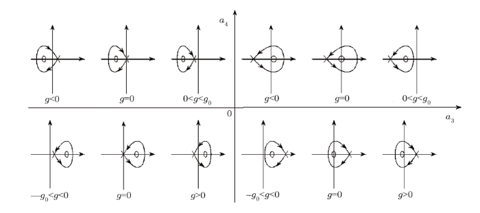
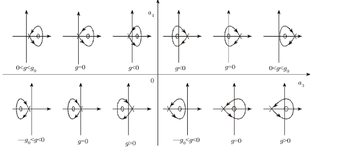
Thus, based on the above analysis, we get the bifurcation phase portraits of Eq. (31) as Figs. 1 and 2.

Fig. 1

New window|Download| PPT slide
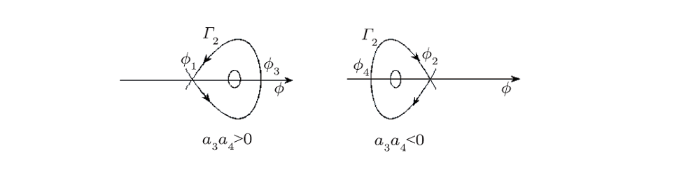
Fig. 1The bifurcation phase portraits of Eq. (31) when $l^{2}+a_{1}ln+a_{2}n^{2}>0$.

Fig. 2

New window|Download| PPT slide
Fig. 2The bifurcation phase portraits of Eq. (31) when $l^{2}+a_{1}ln+a_{2}n^{2}<0$.



Next, due to the qualitative theory of dynamical system, we deduce the traveling wave solutions to Eq. (31). Furthermore, we divide our arguments into two cases.

Case 1 $g=0$.

When $g=0$, Eq. (31) reduces to the system as follows

(36)$\frac{d\phi}{d\xi}=y\,, \nonumber\\ \frac{d y}{d\xi}=\frac{-a_{4}m^{2}\phi^{2}-(l^{2}+a_{1}ln+a_{2}n^{2})\phi}{a_{3}m^{4}}\,.$
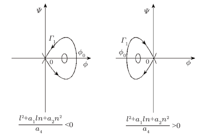
From Figs. 1 and 2, we observe that Eq. (31) has a homoclinic orbits $\Gamma_{1}$ (see Fig. 3).

Fig. 3

New window|Download| PPT slide
Fig. 3Homoclinc orbits when ${a_{3}}/({l^{2}+a_{1}ln+n^{2}})<0$.



In $\phi-y$ plane, $\Gamma_{1}$ is described as

(37) $y^{2}=\frac{2a_{4}m^{2}}{3a_{3}m^{4}}\phi^{3}-\frac{l^{2}+a_{1}ln+a_{2}n^{2}}{a_{3}m^{4}}\phi^{2}\,,\\ \phi\in(0,\phi_{0}) {\rm or} \phi(\phi_{0},0)\,, $
where $\phi_{0}=({3(l^{2}+a_{1}ln+a_{2}n^{2})})/({2a_{4}m^{2}})$.

It follows from Eqs. (36) and (37) that

(38)$\pm\sqrt{\frac{1}{\frac{2a_{4}}{3a_{3}m^{2}}\phi^{3}-\frac{l^{2}+a_{1}ln+a_{2}n^{2}}{a_{3}m^{4}}\phi^{2}}}d\phi=d\xi\,.$
Assuming that $\phi(0)=\phi_{0}$ and integrating Eq. (38) along homoclinic orbit $\Gamma_{1}$, we obtain

(39)$\int_{\phi}^{\phi_{0}}\frac{d s}{\sqrt{{\frac{2a_{4}}{3a_{3}m^{2}}s^{3}-\frac{l^{2}+a_{1}ln+a_{2}n^{2}}{a_{3}m^{4}}s^{2}}}}=\int_{\xi}^{0}d s\,, \;\; \xi<0\,,$
(40)$-\int_{\phi_{0}}^{\phi}\frac{d s}{\sqrt{{\frac{2a_{4}}{3a_{3}m^{2}}s^{3}-\frac{l^{2}+a_{1}ln+a_{2}n^{2}}{a_{3}m^{4}}s^{2}}}}=\int_{0}^{\xi}d s\,,\;\; \xi>0\,.$
From Eqs. (39) and (40), we get

(41)$\phi=\frac{-3(l^{2}+a_{1}ln+a_{2}n^{2})}{a_{4}m^{2}\left[1-\cosh(\eta\xi)\right]}\,, $
(42)$\phi=\frac{-3(l^{2}+a_{1}ln+a_{2}n^{2})}{a_{4}m^{2}\left[1+\cosh(\eta\xi)\right]}, $
where $\eta=\sqrt{-({l^{2}+a_{1}ln+a_{2}n^{2}})/{a_{3}m^{4}}}$.

From Eq. (41) and Eq. (42) and traveling wave transformation

$$A=\phi(\xi)\,,\quad \xi=mX+nY+lT\,,$$

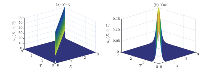
we obtain the solitary wave solutions

(43)$u_{1}(X,Y,T)=\frac{-3(l^{2}+a_{1}ln+a_{2}n^{2})}{a_{4}m^{2}\Bigl[1-\cosh\sqrt{-\frac{l^{2}+a_{1}ln+a_{2}n^{2}}{a_{3}m^{4}}}\xi\Bigr]}, $
(44)$u_{2}(X,Y,T)=\frac{-3(l^{2}+a_{1}ln+a_{2}n^{2})}{a_{4}m^{2}\Bigl[1+\cosh\sqrt{-\frac{l^{2}+a_{1}ln+a_{2}n^{2}}{a_{3}m^{4}}}\xi\Bigr]}. $
See Fig. 4.

Fig. 4

New window|Download| PPT slide
Fig. 4The diagrammatic sketch of the solutions of the case 1 with $m=n=1$, $l=-1$, $a_{1}=a_{2}=0.01$, $a_{3}=-0.01$, $a_{4}=10$. (a) $u_{1}(\xi)$, (b) $u_{2}(\xi)$.



Similarly, we can obtain the other solitary wave solutions

(45)$u_{3}(X,Y,T)=\frac{(l^{2}+a_{1}ln+a_{2}n^{2})\Bigl[-2+\cosh\sqrt{\frac{l^{2}+a_{1}ln+a_{2}n^{2}}{a_{3}m^{4}}}\xi\Bigr]}{a_{4}m^{2}\Bigl[1+\cosh\sqrt{\frac{l^{2}+a_{1}ln+a_{2}n^{2}}{a_{3}m^{4}}}\xi\Bigr]},\\ $
(46)$u_{4}(X,Y,T)=\frac{(l^{2}+a_{1}ln+a_{2}n^{2})\Bigl[2+\cosh\sqrt{\frac{l^{2}+a_{1}ln+a_{2}n^{2}}{a_{3}m^{4}}}\xi\Bigr]}{a_{4}m^{2}\Bigl[-1+\cosh\sqrt{\frac{l^{2}+a_{1}ln+a_{2}n^{2}}{a_{3}m^{4}}}\xi\Bigr]}. $
See Fig. 5.

Fig. 5

New window|Download| PPT slide
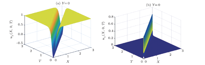
Fig. 5The diagrammatic sketch of the solutions of the case 1 with $m=n=1$, $l=-1$, $a_{1}=a_{2}=a_{3}=0.01$, $a_{4}=1$. (a) $u_{3}(\xi)$, (b) $u_{4}(\xi)$.



Case 2 $g\neq0$.

From Fig. 1 to Fig. 2, we observe that Eq. (31) has a homoclinic orbit $\Gamma_{2}$. See Fig. 6.

Fig. 6

New window|Download| PPT slide
Fig. 6Homoclinc orbits when $0＜-g＜g_{0}$.



In $\phi-y$ plane, $\Gamma_{2}$ is described as

(47) $y^{2}=\frac{2a_{4}m^{2}}{3a_{3}m^{4}}\phi^{3}-\frac{l^{2}+a_{1}ln+a_{2}n^{2}}{a_{3}m^{4}}\phi^{2}-\frac{2g}{a_{3}m^{4}}\phi+2h, \quad \phi\in(\phi_{1},\phi_{3}) {\rm or} \phi\in(\phi_{4},\phi_{2})\,,$
where $h=H(\phi_{i},0)$, $i=1,2,$

$$\phi_{3}=\frac{-(l^{2}+a_{1}ln+a_{2}n^{2})+\sqrt{\Delta}}{2a_{4}m^{2}}\,,\quad \phi_{4}=\frac{-(l^{2}+a_{1}ln+a_{2}n^{2})-\sqrt{\Delta}}{2a_{4}m^{2}}\,,$$

where $\Delta=\sqrt{(l^{2}+a_{1}ln+a_{2}n^{2})^{2}+4a_{4}m^{2}g}$.

It follows from Eqs. (31) and (47) that

(48)$\pm\sqrt{\frac{1}{\frac{2a_{4}m^{2}}{3a_{3}m^{4}}\phi^{3}-\frac{l^{2}+a_{1}ln+a_{2}n^{2}}{a_{3}m^{4}}\phi^{2}-\frac{2g}{a_{3}m^{4}}\phi+2h}}d\phi=d\xi. $
Assuming that $\phi(0)=\phi_{3}$ and integrating Eq. (48) along homoclinic orbit $\Gamma_{2}$, we have

(49)$\int_{\phi}^{\phi_{3}}\frac{1}{\sqrt{{\frac{2a_{4}m^{2}}{3a_{3}m^{4}}s^{3}-\frac{l^{2}+a_{1}ln+a_{2}n^{2}}{a_{3}m^{4}}s^{2}-\frac{2g}{a_{3}m^{4}}s+2h}}}d s=\int_{\xi}^{0}d s,\quad \xi<0, $
(50)$-\int_{\phi_{3}}^{\phi}\frac{1}{\sqrt{{\frac{2a_{4}m^{2}}{3a_{3}m^{4}}s^{3}-\frac{l^{2}+a_{1}ln+a_{2}n^{2}}{a_{3}m^{4}}s^{2}-\frac{2g}{a_{3}m^{4}}s+2h}}}d s=\int_{0}^{\xi}d s\,,\quad \xi>0\,.$
By Eqs. (49) and (50), we obtain

(51)$u_{5}(X,Y,T)=\frac{-1}{4a_{4}m^{2}}\bigl\{-(l^{2}+a_{1}ln+a_{2}n^{2})+5\Delta-[(l^{2}+a_{1}ln+a_{2}n^{2})-\Delta]\cosh(\gamma\xi)\bigr\} \csc^{2}h\Bigl(\frac{\gamma}{2}\xi\Bigr),\\ $
(52)$u_{6}(X,Y,T)=\frac{1}{4a_{4}m^{2}}\Bigl\{-(l^{2}+a_{1}ln+a_{2}n^{2})+5\Delta+[(l^{2}+a_{1}ln+a_{2}n^{2})-\Delta]\cosh(\gamma\xi){\rm sec}^2h\Bigl(\frac{\gamma}{2}\xi\Bigr)\Bigr\},$
where $\Delta=\sqrt{(l^{2}+a_{1}ln+a_{2}n^{2})^{2}+4a_{4}m^{2}g}$, $\gamma=\sqrt{{\Delta}/{-a_{3}m^{4}}}$.

See Fig. 7.

Fig. 7

New window|Download| PPT slide
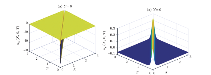
Fig. 7The diagrammatic sketch of the solutions of the case 2 with $m=n=1$, $l=-1$, $a_{1}=a_{2}=0.1$, $a_{3}=-0.01$, $a_{4}=10$, $g=0.1$. (a) $u_{5}(\xi)$, (b) $u_{6}(\xi)$.



Similarly, we can deduce that solitary wave solutions

(53)$u_{7}(X,Y,T)=\frac{1}{4a_{4}m^{2}}\{(l^{2}+a_{1}ln+a_{2}n^{2})+5\Delta+[-(l^{2}+a_{1}ln+a_{2}n^{2})+\Delta]\cosh(\delta\xi)\}\csc h^{2}\Bigl(\frac{\delta}{2}\xi\Bigr), $
(54)$u_{8}(X,Y,T)=\frac{1}{4a_{4}m^{2}}\{-(l^{2}+a_{1}ln+a_{2}n^{2})-5\Delta+[-(l^{2}+a_{1}ln+a_{2}n^{2})+\Delta]\cosh(\delta\xi)\}{\rm sec} h^{2}\Bigl(\frac{\delta}{2}\xi\Bigr), $
where $\delta=\sqrt{{\Delta}/{a_{3}m^{4}}}$.

See Fig. 8.

Fig. 8

New window|Download| PPT slide
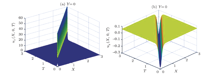
Fig. 8The diagrammatic sketch of the solutions of the case 2 with $m=n=1$, $l=-1$, $a_{1}=a_{2}=0.1$, $a_{3}=0.01$, $a_{4}=10$, $g=0.1$. (a) $u_{7}(\xi)$, (b) $u_{8}(\xi)$.



From Figs. 4, 5, 7, 8, it can be seen that these traveling wave solutions are all Rossby solitary waves.

4 Conclusion

In this paper, firstly, we derive a new $(2+1)$-dimensional generalized Boussinesq equation with generalized beta effect from the barotropic potential vorticity equation by using methods of the multiple scales and weak nonlinear perturbation expansions. Secondly, borrowing from the ideas of Ref. [44], we present the dynamical analysis and obtain exact traveling wave solutions of the new generalized Boussinesq equation. Finally, we show the simulations of the bifurcation phase portraits and the exact traveling wave solutions under some conditions of some parameters.Indeed, in our contribution, Eq. (30) is equivalent to the following ordinary differential equation

$$P\phi^{\prime\prime}+Q\phi+R\phi^{2}=g\,,$$

where $P$, $Q$, and $R$ are constants and $g$ is the integral constant.

However, in Ref. [44], under traveling wave transformation, we observe that the authors investigated ordinary differential equation

(55)$P\phi^{\prime\prime}+Q\phi+R\phi^{3}=0\,,$
and considered the integral constant $g=0$. Thus, based on the ideas of our paper, we can also investigate the dynamical analysis and obtain exact traveling wave solutions of Eq. (55) in the future research.

Acknowledgments

We would like to thank two anonymous reviewers for their comments, which have helped to improve the presentation of this manuscript substantially.

Reference View Option By original order
By published year
By cited within times
By Impact factor

[1] Q. S. Liu, R. G. Zhang, L. G. Yang, Phys. Lett. A. 383 ( 2019) 514.
[Cited within: 2]

[2] R. G. Zhang and L. G. Yang, Dynam. Atmos. Oceans.85 ( 2019) 16.


[3] Y. W. Ren, M. S. Tao, H. H. Dong, H. W. Yang, Adv. Differ. Equ.2019 ( 2019) 13.


[4] C. Fu, C. N. Lu, H. W. Yang, Adv. Differ. Equ.2018 ( 2018) 56.


[5] C. N. Lu, C. Fu, H. W. Yang, Appl. Math. Comput.327 ( 2018) 104.
[Cited within: 1]

[6] L. Fu, Y. D. Chen, H. W. Yang, Mathematics.7 ( 2019) 41.


[7] H. W. Yang, J. C. Sun, C. Fu , Commun. Nonlinear Sci. Numer. Simulat. 71 ( 2019) 187.
[Cited within: 1]

[8] M. Nezlin and E. Snezhkin , Springer Series in Non-Linear Dynamics
Springer-Verlag,Berlin ( 1993).
[Cited within: 1]

[9] R. R. Long, J. Atmos. Sci.21( 1964) 197.
[Cited within: 1]

[10] D. J. Benney, J. Math. Phys.45 ( 1966) 52.


[11] J. P. Boyd, J. Phys. Ocean.10( 1980) 1699.


[12] K. C. Le and L. T. K. Nguyen , Int. J. Eng. Sci. 83 ( 2014) 117.


[13] M. Wadati , J. Phys. Soc. Jpn. 34 ( 1973) 1289.


[14] L. G. Redekopp and P. D. Weidman, J. Atmos. Sci.35 ( 1978) 790.


[15] M. C. Li, Adv. Atmos. Sci.4 ( 1987) 125.


[16] J. G. Charney and D. M. J. Straus, J. Atmos. Sci.37 ( 1980) 1157.


[17] H. Ono , J. Phys. Soc. Jpn. 50 ( 1981) 2757.


[18] H. W. Yang, Q. F. Zhao, B. S. Yin, H. H. Dong, Abst. Appl. Anal.2013 ( 2013) 597807.


[19] H. W. Yang, D. Z. Yang, Y. L. Shi, B. S. Yin, Dynam. Atmos. Oceans.71 ( 2015) 21.


[20] K. C. Le and L. T. K. Nguyen, Nonlinear Dynam.81 ( 2015) 659.
[Cited within: 1]

[21] B. B. Kadomtsev and V. I. Petviashvili, Sov. Phys. Dokl.15 ( 1970) 539.
[Cited within: 1]

[22] M. D. Groves and S. M. Sun , Arch. Rat. Mech. Anal. 188 ( 2008) 1.
[Cited within: 1]

[23] E. Infeld and G. Rowlands, , Nonlinear Waves, Solitons and Chaos
Cambridge University Press Cambridge( 2001).
[Cited within: 1]

[24] V. E. Zakharov and E. A. Kuznetsov, Sov. Phys.39( 1974) 285.
[Cited within: 1]

[25] M.J Ablowitz and A. Clarkson P, Solitons, . Nonlinear Evolution Equations and Inverse Scattering
Cambridge University Press Cambridge( 1991).
[Cited within: 1]

[26] R. S. Johnson, J. Fluid. Mech.323 ( 1996) 65.
[Cited within: 1]

[27] D. E. Mitsotakis, Math. Comput. Simulat.80 ( 2009) 860.
[Cited within: 1]

[28] G. A. Gottwalld, ( arXiv:nlin/0312009v1 2003 2003) 1.
[Cited within: 1]

[29] H. W. Yang, Z. H. Xu, X. R. Feng, et al.., ( Adv. Differ. Equ.2016 2016) 167.
[Cited within: 1]

[30] H. Yang, X. Chen, M. Guo, Y. Chen, ( Nonlinear Dynam.91 2018) 2019.
[Cited within: 1]

[31] R. G. Zhang, L. G. Yang, J. Song, ( Nonlinear Dynam.90 2017) 815.
[Cited within: 1]

[32] R. G. Zhang, L. G. Yang, J. Song, ( Comput. Math. Appl.73 2017) 1996.
[Cited within: 1]

[33] W. X. Ma and B. Fuchssteiner , Int. J. Nonlinear Mech. 31 ( 1996) 329.
[Cited within: 1]

[34] J. Manafian and M. F. Aghdaei , Eur. Phys. J. Plus. 131 ( 2016) 97.
[Cited within: 1]

[35] A. M. Wazwaz , Commun. Nonlinear Sci. Numer. Simulat. 10 ( 2005) 597.
[Cited within: 1]

[36] W. X. Ma and Y. You , Trans. Amer. Math. Soc. 357 ( 2005) 1753.
[Cited within: 1]

[37] C. Lin and X. Zhang , Commun. Nonlinear Sci. Numer. Simul. 12 ( 2007) 636.
[Cited within: 1]

[38] S. Talaat and Aly El-Danaf , Commun. Nonlinear Sci. Numer. Simul. 13 ( 2008) 554.
[Cited within: 1]

[39] W. X. Ma and J. H. Lee, , Chaos Solitons & Fractals 42 ( 2009) 1356.
[Cited within: 1]

[40] W. X. Ma and M. Chen, ( Appl. Math. Comput.215 2009) 2835.
[Cited within: 1]

[41] S. Haq and M. Uddin, ( Appl. Math. Model.33 2009) 3442.
[Cited within: 1]

[42] Z. Z. Ganji, D. D. Ganji, Y. Rostamiyan, ( Appl. Math. Model.33 2009) 3107.
[Cited within: 1]

[43] Z. Y. Zhang, Z. H. Liu, X. J. Miao, Y. Z. Chen, ( Appl. Math. Comput.216 2010) 3064.
[Cited within: 1]

[44] Z. Y. Zhang, Z. H. Liu, X. J. Miao, Y. Z. Chen, ( Phys. Lett. A375 2011) 1275.
[Cited within: 5]

[45] W. X. Ma and Z. Zhu, ( Appl. Math. Comput.218 2012) 11871.
[Cited within: 1]

[46] Z. Y. Zhang, Y. X. Li, X. J. Liu , Commun. Nonlinear Sci. Numer. Simulat.16 ( 2011) 3097.
[Cited within: 1]

[47] X. J. Miao and Z. Y. Zhang , Commun. Nonlinear Sci. Numer. Simulat. 16 ( 2011) 4259.
[Cited within: 1]

[48] Z. Y. Zhang, X. Y. Gan, D. M. Yu, Y. H. Zhang, ( Commun. Theor. Phys.57 2012) 764.
[Cited within: 1]

[49] O. Tasbozan, Y. Cenesiz, A. Kurt , Eur. Phys. J. Plus. 131 ( 2016) 244.
[Cited within: 1]

[50] M. Uddin, ( Appl. Math. Model.38 2014) 135.
[Cited within: 1]

[51] Z. Y. Zhang, ( Pramana-J. Phys.82 2014) 1011.
[Cited within: 1]

[52] X. Lü, S. T. Chen, W. X. Ma, ( Nonlinear Dynam.86 2016) 523.
[Cited within: 1]

[53] W. X. Ma, Z. Y. Qin, X. Lü, ( Nonlinear Dynam.84 2016) 923.
[Cited within: 1]

[54] X. Lü, and W. X. Ma, Nonlinear Dynam.85 ( 2016) 1217.
[Cited within: 1]

[55] H. M. Wang and G. W. Yan, ( Appl. Math. Model.40 2016) 5139.
[Cited within: 1]

[56] H. M. Wang, ( Appl. Math. Model.45 2017) 1.
[Cited within: 1]

[57] J. Pedlosky, , Geophysical Fluid Dynamics
Springer-Verlag, Berlin ( 1987).
[Cited within: 1]

[58] J. Song and L. G. Yang, ( Chin. Phys. B18 2009) 2873.
[Cited within: 1]

[59] P. Caillol and R. H. Grimshaw, ( Stud. Appl. Math.120 2008) 35.
[Cited within: 1]