M. Awais^,2,*, S. Bilal¹, M. Y. Malik^2,3, Khalil -ur-Rehman¹1 Department of Mathematics, AIR University, Sector E-9, Air Complex, Islamabad 44000, Pakistan
2 Department of Mathematics,College of Sciences, King Khalid University, Abha 61413, Saudi Arabia
3 Department of Mathematics, Quaid-i-Azam University, Islamabad 44000, Pakistan

Corresponding authors: *E-mail:smbilal@math.qau.edu.pk

Received:2018-08-15Accepted:2018-11-20Online:2019-09-1


Abstract
Current exertion is made to depict and search out the flow features imparted to viscid fluid flow over a rotational disk. Impression of magnetic field with rotating fluid is generated by interacting it in radial direction. Nano structured particles with magnetized fluid are also incorporated in the upshot of chemical reaction and absorptive/generative heat induction. Von Kumaran procedure is executed to obtain flow narrating differential expressions. Flow pattern regarding thermal, momentum profiles are comprehended with the support of shooting method and Runge-Kutta methods. Furthermore, to get more realistic view of result description computational algorithm is modified by improving Runge-Kutta coefficients with Cash and Carp method. The aspects of flow controlling parameters like momentum slip parameter, magnetic strength parameter, Brownian motion parameter, thermophoresis parameter are adorned in sketches. Findings of these architects are accumulated in conclusion section.
Keywords： heat generation/absorption;viscous fluid model;nanoparticles;rotating disk;Navier slip;Cash and Carp method


PDF (1227KB)MetadataMetricsRelated articlesExportEndNote|Ris|BibtexFavorite
Cite this article
M. Awais, S. Bilal, M. Y. Malik, Khalil -ur-Rehman. Numerical Analysis of Magnetohydrodynamic Navier's Slip Visco Nanofluid Flow Induced by Rotating Disk with Heat Source/Sink. [J], 2019, 71(9): 1075-1083 doi:10.1088/0253-6102/71/9/1075

Nomenclature






New window|CSV

1 Introduction

Mechanically fluid flow generated by rotating disc has attained prodigious attention of scientists and engineers in the recent past due to its superb applications in geophysics, aeronautical science, crystal growth process, thermal power generating system etc. Significant geophysical applications of rotating disk incorporate the subject of earth's revolution in its orbit and magma movement. Other essential mechanical applications of rotating disk involve air purifying devices, centrifugal filtration process, biological devices, food manufacturing, rotating machinery, aero spaced field and in electrified power generated surroundings. Von Karman^[1] coined the idea of rotating disc discussing fluid flow induced by it. Lately, numerical investigation on combined features of thermal and concentration transfer flow of viscid fluid by way of Darcy rotating disc was executed by Turkyilmozoglu and Senel.^[2] Inspection of non-Newtonian liquid induced by rotated disc in permeable media was discussed by Guram and Anwar.^[3] Rashidi et al.^[4] addressed the entropy generated in viscous flow over rotated disk. Turkyilmozoglu^[5] discoursed the flow generated by rotated disk in the attendance of nanostructures. Mustafa et al.^[6] investigated dynamics of nanoliquid due to stretchable disk. Sheikholeslami et al.^[7] studied viscous nanoliquid flow due to inclining rotated disk geometry.

At present there is remarkable requirement of electronic devices in numerous industrial progressions. But recession in thermal conductivity of these equipments has abridged their valuable acknowledgement. Such confined products can be well-ordered by mounting new heat transfer liquids in laboratories. These engineered liquids can be prepared by accruing small solid size subdivisions into base fluids in order to aggrandize the thermophysical capability of host fluids. Researchers have concluded that with the inclusion of these small size particles the issues related to low thermal conductivity of fluids in thermal frameworks has been reduced. In view of these characteristics and promising utility nano-fluids are capitalized in thermal engineering, heat exchangers, chemical progression, cancer psychoanalysis and biomedicine etc. Enriched heat transferal proficiency can be engaged to many conspicuous solicitations comprising chilling of microelectronics such as microchips in computer processors, space refrigerating, improving the adeptness of hybrid powered engines, transformers oil cooling, and numerous others. Choi^[8] shared the idea of nanofluids imparts as material for enrichment of thermal conductance. This characteristic of nanofluids has led it to diverse mechanical and biomedical uses such as in frosted engine, reducing agent for drag in refrigeration, chillers, oil engine transferal, heating and cooling of buildings, in exhaustion of boiler, fueled gas recovery, lubrication, reducing temperature in electronics, microwaved tubes, highly-powered lasers, drillers, transformer cooling oil, nuclear systems cooling and solar hydral heating. An extensive investigation of convectional transmission in this fluid was completed by Buongiorno.^[9] Chen et al.^[10] suggested a methodology to calculate the thermal conductivity of fluid comprising of nano-sized structures constructed on their rheological features. An extensive analysis of boundary layered flow over an exponential stretchable surface comprising of nanostructures was executed by Nadeem et al.^[11] Significance of nanofluid in increasing the heavy-duty engine and automotive cooling rates was elucidated by Peyghambarzadeh et al.^[12]

The imposition or interaction of magnetic field with dynamical flows is renowned as magnetohydrodynamics and such fluids are called magnetized fluids. The fundamental concept of appliance of magnetic field is to instigate magnetic currents in movable conducting liquids, which consequently generates a resistive force on the fluid. So The analysis of fluid flows with the interaction of magnetic field has engrossed substantive focus of investigators. Such considerations is due to its utilization in various mechanical, industrial and technological processes i.e. enhanced oil recovery, magnetohydrodynamic generators, electronic packages, pumps, thermal insulators, flow meters, power generation, etc. Furthermore, the appliance of magnetic field molds the orientation of interacting fluid molecules and also controls the intensity of flow phenomenon. Due to above mentioned importance researchers are considering fluid flows in various orientations under the effect of applied magnetic field. Few recent works in this direction is described as follows. Alfven^[13] was the first who described the class of MHD waves also known as Alfven waves. In fluid dynamics, magnetic flow of non-Newtonian liquids was initially examined by Sarpkaya^[14] and then this work was further prolonged by many investigators. Liao^[15] acquired HAM solution for non-Newtonian flow regime by way of linearly stretchable geometry under the account of magnetic field. He suggested that magnetic parameter amplifies the frictional drag coefficient. MHD stagnant flow incorporated with chemical reactive species immerse in Darcy stretchable configuration was deliberated by Mabood et al.^[16] Malik et al.^[17] configured the physical impact of MHD on hyperbolic tangent liquid over a stretchable cylindrical configuration. Akbar et al.^[18] computationally analyzed Powel-Eyring liquid under the inspiration of magnetic field over a stretchable surface. Hayat et al.^[19] addressed the analysis on magnetohydrodynamic flow of fluid on a rotating disk with slip effects. Gireesha^[20] contemplated electrically conducting three dimensional Casson fluid under the impact of non-linear radiation and double diffusion aspect. They attained the computational solution of the problem by obliging Runge-Kutta method. Magnetohydrodynamic Falkner-Skan flow of a Casson nanofluid in the presence of non-linear thermal radiation and variable thermo-physical properties are investigated by Archana et al.^[21] Gireesha^[22] depicted analysis to scrutinize the laminar, boundary layer stagnation point flow of a nanofluid over a permeable, vertical stretching sheet by capitalizing the effects of Brownian motion with thermophoresis in the presence of uniform magnetic field, non-uniform source/sink and chemical reaction. Kumar et al.^[23] adumbrated the thermophysical features of Prandtl fluid over a Riga plate in the presence of magnetic field and chemically reactive species. Archana et al.^[24] interrogated the features imparted in three dimensional Maxwell fluid by non-linear radiative flux and magnetic field.

Aforesaid extensive depictions witnesses that so far very less literature regarding the features of fluid prompted by rotating rigid disk in the attendance of velocity slip, magnetic field, generative/absorptive heat and chemical reactive species are not taken into account. The generally accepted fundamental are utilized to obtain the ultimate mathematical equations. For solution purpose, a numerical method is implemented by improving it to Cash and Carp procedure. Regarding structure of the manuscript is concerned, Sec.1 is all about literature survey while Sec.2 is made to offer mathematical treatment subject to viscous nanofluid flow due to rotating disk. The numerical scheme for present fluid flow problem is given in Sec.3. The attained interpretations are shared in Sec.4 while the corresponding graphs are given in Sec.5. The key outcomes are abridged in Sec.6.

2 Mathematical Formulation

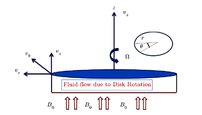
Let us assume 2-dimensional, laminar, magneto hydrodynamic boundary layered flow of an incompressible viscous nanoliquid yields by rotational disk with slip condition. The disk at $z=0$ rotates with angular velocity ${v^z}$. Velocity component along radial $r$-direction is ${v^r}$, ${v^\theta }$ is the velocity component along tangential $\theta$-direction and ${v^z}$ is velocity component along axial $z$-direction. An unvarying magnetic strength ${B_0}$ is employed in the $z$-direction. Flow situation is taken with chemical reactive species and generative/absorptive heat effects. The physical structure of flow regime via rotating disk is elucidated in accompanied Fig.1.

Fig.1

New window|Download| PPT slide
Fig.1(Color online) Schematic diagram of rotating disk.



In the current situation the governing boundary layer equations take the following forms

(1)$\frac{{\partial {v^r}}}{{\partial r}} + \frac{{{v^r}}}{r} + \frac{{\partial {v^z}}}{{\partial z}}\, = \,0,$
(2)${v^r}\frac{{\partial {v^r}}}{{\partial r}} - \frac{{{v^r}^2}}{r} + {v^z}\frac{{\partial {v^r}}}{{\partial z}}\,\, = \,\, - \frac{1}{{{\rho _f}}}\frac{{\partial p}}{{\partial r}} + \nu \Bigl( {\frac{{{\partial ^2}{v^r}}}{{\partial {r^2}}} + \frac{1}{r}\frac{{\partial {v^r}}}{{\partial r}} - \frac{{{v^r}}}{{{r^2}}}\frac{{{\partial ^2}{v^r}}}{{\partial {z^2}}}} \Bigr) - \frac{{\sigma B_0^2}}{{{\rho _f}}}{v^r},$
(3)${v^r}\frac{{\partial {v^\theta }}}{{\partial r}} + \frac{{{v^r}{v^\theta }}}{r} + {v^z}\frac{{\partial {v^z}}}{{\partial z}}\,\, = \,\,\nu \Bigl( {\frac{{{\partial ^2}{v^\theta }}}{{\partial {r^2}}} + \frac{1}{r}\frac{{\partial {v^\theta }}}{{\partial r}} - \frac{{{v^\theta }}}{{{r^2}}}\frac{{{\partial ^2}{v^\theta }}}{{\partial {z^2}}}} \Bigr) - \frac{{\sigma B_0^2}}{{{\rho _f}}}{v^\theta },$
(4)${v^r}\frac{{\partial {v^z}}}{{\partial r}} + {v^z}\frac{{\partial {v^z}}}{{\partial z}}\,\, = \, - \frac{1}{{{\rho _f}}}\frac{{\partial p}}{{\partial r}} + \,\nu \Bigl( {\frac{{{\partial ^2}{v^z}}}{{\partial {r^2}}} + \frac{1}{r}\frac{{\partial {v^z}}}{{\partial r}} + \frac{{{\partial ^2}{v^z}}}{{\partial {z^2}}}} \Bigr),$
(5)${v^r}\frac{{\partial \bar T }}{{\partial r}} + {v^z}\frac{{\partial \bar T }}{{\partial z}}\,\,\,\,\, = \,\,\,\,\,\alpha \Bigl( {\frac{{{\partial ^2}\bar T }}{{\partial {r^2}}} + \frac{1}{r}\frac{{\partial \bar T }}{{\partial r}} + \frac{{{\partial ^2}\bar T }}{{\partial {z^2}}}} \Bigr)\\ \quad\quad\,\,\,+ \frac{{{{\left( {\rho c} \right)}_p}}}{{{{\left( {\rho c} \right)}_f}}}\Bigl[ {{D_B}\Bigl( {\frac{{\partial \bar T }}{{\partial r}}\frac{{\partial \bar C }}{{\partial r}} + \frac{{\partial \bar T }}{{\partial z}}\frac{{\partial \bar C }}{{\partial z}}} \Bigr) + \frac{{{D_T}}}{{{T_\infty }}}\Bigl( {{{\Bigl( \frac{{\partial \bar T }}{\partial r}\Bigr)^2}} + {{\Bigl( \frac{{\partial \bar C }}{\partial r}\Bigr)^2}}} \Bigr)} \Bigr] + \frac{{{Q_0}}}{{{c_p}\rho }}\left( {\bar T - {{\bar T }_\infty }} \right),$
(6)${v^r}\frac{{\partial \bar C }}{{\partial r}} + {v^z}\frac{{\partial \bar C }}{{\partial z}}\,\, = \,\,{D_B}\Bigl( {\frac{{{\partial ^2}\bar C }}{{\partial {r^2}}} + \frac{1}{r}\frac{{\partial \bar C }}{{\partial r}} + \frac{{{\partial ^2}\bar C }}{{\partial {z^2}}}} \Bigr) + \frac{{{D_T}}}{{{{\bar T }_\infty }}}\Bigl[ {\frac{{{\partial ^2}\bar T }}{{\partial {r^2}}} + \frac{1}{r}\frac{{\partial \bar T }}{{\partial r}} + \frac{{{\partial ^2}\bar T }}{{\partial {z^2}}}} \Bigr] - K\left( {\bar C - {{\bar C }_\infty }} \right).$
The corresponding boundary conditions are

(7)${v^r}={{\rm A}_1}\frac{{\partial {v^r}}}{{\partial z}}, \quad{v^\theta }= r{\rm{ }}\Omega + {{\rm A}_1}\frac{{\partial {v^\theta }}}{{\partial z}},\quad {v^z} = 0,\\ \bar T = {\bar T _w} + {{\rm A}_2}\frac{{\partial \bar T }}{{\partial z}},\quad \bar C = {\bar C _w} \quad{\rm{at}}\quad z=0,$
(8)$v^r\rightarrow 0,\quad v^{\theta}\rightarrow 0,\quad \bar{T}\rightarrow\bar{T}_{\infty}, \nonumber\\ \bar{C}\rightarrow\bar{C}_{\infty}\quad {\rm as}\quad z\rightarrow\infty, $
where $\nu =\mu /{\rho _f}$ is the kinematic viscosity, $\mu $ is the dynamic viscosity, $\sigma $ is the electrical conductivity of the fluid, $p$ denotes the pressure, $\rho $ is the density, ${\rho _f}$ is the density of the base fluid, ${\left( {\rho c} \right)_p}$ is the effective heat capacity of nanoparticles, $\alpha =k/{\left( {\rho c} \right)_f}$ is the thermal diffusivity, ${\left( {\rho c} \right)_f}$ is the heat capacity, $\bar T $ is the temperature, $\bar C $ is the concentration, ${D_B}$ is the Brownian diffusion coefficient, $D_T$ is the thermophoretic diffusion coefficient, ${{\rm A}_1}$ is the velocity slip constant, ${{\rm A}_2}$ is the temperature jump, ${\bar T _w}$ is the surface temperature, ${\bar T _\infty }$ is the ambient temperature, ${\bar C _w}$ is the surface concentration, ${\bar C _{\infty}}$ is the ambient concentration, ${Q_0}$ is the thermal generation coefficient, and $K$ is the rate of chemical reactive species.

Now the subsequent dimensionless variables are as under:

(9)${v^r}=r\Omega {f'}\left(\eta \right),\quad{v^\theta }=r\Omega g(\eta), \quad {v^z}=- \sqrt {2\Omega \nu}f(\eta)\\ T(\eta )=\frac{{\bar T-{{\bar T }_\infty }}}{{{{\bar T }_w} - {{\bar T }_\infty }}}, \quad C(\eta )=\frac{{\bar C - {{\bar C }_\infty }}}{{{{\bar C }_w} - {{\bar C }_\infty }}}, \quad \eta=\sqrt{\frac{{2\Omega }}{\nu }}z.$
Now Eq.(1) is fully identicalized and Eqs.(2)-(8) take the accompanied forms

(10)$2f^{\prime\prime\prime}(\eta)+2f(\eta ){f^{\prime\prime}}(\eta )-{\left({{f^{\prime}} (\eta)}\right)^2}+{\left({g(\eta)}\right)^2}-\beta{f^{\prime}}(\eta)=0,$
(11)$2{g^{\prime\prime}}\left(\eta\right)+2f(\eta){g'}\left(\eta\right)-2g\left(\eta\right){f'} \left(\eta\right)-{\beta^2}g(\eta)=0,$
(12)${T^{\prime\prime}}(\eta)+Pr(f(\eta){T'}(\eta)+Nb{T'}(\eta){C'}(\eta)\\ \quad\quad\,\,\,\,+Nt{T^{\prime\prime}}(\eta)+{h_g}T(\eta))=0,$
(13)${C^{\prime\prime}}(\eta)+Scf{C'}(\eta)+\frac{{{N_t}}}{{{N_b}}}{T^{\prime\prime}}(\eta) -{\delta_c}ScC(\eta) =0,$
the associate boundary conditions are given as:

(14)$f\left( \eta \right)=0,\quad{f'}\left( \eta \right)=\lambda {f^{\prime\prime}}\left( \eta \right),\\ g\left( \eta \right)=1 + \lambda {g'}\left( \eta \right),\quad{\rm{at }}\quad\eta=0,\\ T\left( \eta \right)=1 + {\lambda _1}{T'}\left( \eta \right),\quad{C'}\left( \eta \right) = 1,\quad{\rm{at}}\quad\eta=0,\\ {f'}\left( \eta \right) \to 0,\quad g\left( \eta \right) \to 0,\quad T\left( \eta \right) \to 0,\\ C\left( \eta \right) \to 0,\quad{\rm{as}}\quad\eta \to \infty . $
Here $\beta $ is the magnetic field parameter, $\lambda $ is the velocity slip parameter, ${\lambda _1}$ thermal slip parameter, $Pr $ is the Prandtl number, $Nb$ is the Brownian motion parameter, $Nt$ is the thermophoresis parameter, $H$ is the heat generation/absorption parameter, ${\delta _c}$ is the chemical reaction parameter and $Sc$ is the Schmidth number. These variables are described as follows:

(15)$\beta =\frac{{\sigma {B_0}^2}}{{{\rho _f}\Omega }},\quad\lambda=L\sqrt {\frac{{2\bar \Omega }}{\nu }}, \quad Nb=\frac{{{{\left( {\rho c} \right)}_p}}}{{{{\left( {\rho c} \right)}_f}}}\frac{{({{\bar T}_w} - {{\bar T}_\infty }){D_T}}}{{{{\bar T}_\infty }\nu }},\\ {h_g}=\frac{{{Q_0}}}{{2\Omega \rho {c_p}}},\quad Sc=\frac{\alpha }{{{D_B}}},\quad Pr=\frac{\nu }{\alpha},\\ Nt=\frac{{{{\left( {\rho c} \right)}_p}}}{{{{\left( {\rho c}\right)}_f}}}\frac{{({{\bar C}_w} - {{\bar C}_\infty }){D_B}}}{\nu },\quad{\delta _c}=\frac{\nu }{{2\Omega {D_B}}}{R_0}. $
The shear stress rate coefficient, local convectional transmission coefficient and local massive flux magnitude are defined as:

(16)$ {\left( {{{{\mathop{ Re}\nolimits} }_{\bar r}}} \right)^{{1}/{2}}}\,{C_F}\,\, = \,\,{f^{\prime\prime}}(\eta )\quad{\rm{ at }}\quad\zeta = {\rm{0}},\\ {\left( {{{{\mathop{ Re}\nolimits} }_{\bar r}}} \right)^{{1}/{2}}}\,{C_G}\,\, = \,\,\,g(\eta )\quad{\rm{ at }}\quad\zeta = {\rm{0}},\\ {\left( {{{{\mathop{ Re}\nolimits} }_{\bar r}}} \right)^{{{ - 1}}/{2}}}\,Nu\, = \, - T(\eta )\quad{\rm{ at }}\quad\zeta = {\rm{0}},\\ {\left( {{{{\mathop{ Re}\nolimits} }_{\bar r}}} \right)^{{{ - 1}}/{2}}}\,Su\, = \, - C(\eta )\quad{\rm{ at }}\quad\zeta = {\rm{0}}. $
in which ${ Re}^r={(\Omega r)^r}/{2\nu}$.

3 Numerical Scheme

As the consequential partial differential expressions of this problem are transformed into ordinary differential equation after applying suitable transformation. But these governing ordinary differential equations (Eqs.(11), (12), and (13)) are highly nonlinear and hard to control their analytical solutions. Keeping in mind the end goal to unravel this system with associated boundary conditions we must solve it i.e. Eq.(14) by numerically. There are many numerical methods which can solve this problem but we solve this problem by shooting technique with RKF-method. For further accuracy of computed results an improvement is made by adding the coefficient of RKF method by Cash and Carp method. Hence first governing boundary value expressions are transmuted into initial value problem, thus governing equations are re-written as

(17)${f^{\prime\prime\prime}} = \frac{1}{2}{f^{'2}} - f{f^{\prime\prime}} + \frac{1}{2}{g^2} + \frac{1}{2}M_f^2f,$
(18)${g^{\prime\prime}} = \frac{1}{2}M_f^2g + g{f'} - f{g'},$
(19)${T^{\prime\prime}} = - \mathop {Pr }({fT' + \,Nb{T'}{C'} + Nt{T^{'2}} + {h_g}T}),$
(20)${C^{\prime\prime}} = - ScPr (f{C'} - {\delta _c}C) - \frac{{Nt}}{{Nb}}{T^{\prime\prime}}.$
To find the numerical solution of these equations by Runge-Kutta scheme, first these equations should be transmuted into system of seven linearized ordered equations with seven unknowns, by letting

(21)${s_1} = f,\quad {s_2} = {f'},\quad {s_3} = {f^{\prime\prime}},\\ {s_4} = g,\quad {s_5} = {g'},\quad {s_6} = T,\\ {s_7} = {T'},\quad {s_8} = C,\quad {s_9} = {C'}, $
under new variables defined in Eq.(21), are given

(22)$\left[ \begin{array}{l} s_1^{'}\\ s_2^{'}\\ s_3^{'}\\ s_4^{'}\\ s_5^{'}\\ s_6^{'}\\ s_7^{'}\\ s_8^{'}\\ s_9^{'} \end{array} \right] = \left[ \begin{array}{l} {s_2}\\ {s_3}\\ _{\frac{1}{2}{{({s_2})}^2} - {s_1}{s_3} + \frac{1}{2}{{({M_f})}^2}{s_1} + \frac{1}{2}{s_4}}\\ {s_5}\\ _{\frac{1}{2}{{({M_f})}^2}{s_4} + {s_2}{s_5} - {s_1}{s_5}}\\ {s_7}\\ _{ - Pr \left( {{s_1}{s_7} + Nb{s_6}{s_9} + Nts_7^2 - {h_g}{s_6}} \right)}\\ {s_9}\\ _{ - ScPr \left( {{s_1}{s_9} - {\delta _c}{s_8}} \right) - \frac{{{N_t}}}{{{N_b}}}s_7'} \end{array} \right]. $
The associated boundary conditions from Eq.(14) in new forms are defined in Eq.(22), take the form

(23)${s_1}(\eta) = 0\,,\quad {s_2}(\eta) = \lambda {s_3}(\eta)\,,\\ {s_4}(\eta) = 1+\lambda {s_5}(\eta){\rm at}\eta\rightarrow0\,,\\ {s_6}(\eta) = 1 + {\lambda _1}{s_7}{\rm{(\eta)}},\quad{s_8}(\eta) =1{\rm at}\eta\rightarrow0\,,\\ {s_2}(\eta)\rightarrow0,\quad s_4(\eta)\rightarrow0,\quad s_6(\eta)\rightarrow0\,,\\ s_8(\eta)\rightarrow0{\rm as}\eta\rightarrow\infty\,. $
To compute the first order differential equations presented in Eq.(23)-(29) seven initial restrictions must be identifiable, but the initial conditions at $s_3$, $s_5$, and $s_7$ are not mentioned. Though, the boundary conditions $s_2(\eta)$, $s_4(\eta)$, and $s_6(\eta)$ are recommended at $\eta\rightarrow\infty$ Thus, these boundary restrictions are used to capitalize three missed initial restrictions. Now, letting the missing initial conditions by $\omega_1$, $\omega_2$, $\omega_3$, and $\omega_4$, it converts the given boundary conditions into initial conditions, new conditions are defined as:

(24)${s_1}(0) = 0\,,\quad {s_2}(0) = \lambda {s_3}(0)\,,\\ {s_3}(0)={\omega _1}\text{(unknown initial condition)}\,,\\ {s_4}(0) = 1 + \lambda {s_5}{\rm{(0)}},\\ {s_5}(0) = {\omega _2}\text{(unknown initial condition)}\,, \\ {s_6}(0) = 1 + {\lambda _1}{s_7}{\rm{(0)}},\\ {s_7}(0) = {\omega _3}\text{(unknown initial condition)}\,,\\ {s_8}(0) = 1,\\ {s_9}(0) = {\omega _4}\text{(unknown initial condition)}\,. $
Initially, the values of $\omega_1$, $\omega_2$, $\omega_3$, and $\omega_4$ are chosen $-1, -1, -1$, and $-1$ respectively. Now solve this system of seven first order ordinary differential equation with initial conditions, the Runge-Kutta-Fehlberg method is used. The Runge-Kutta $4^{\rm th}$ and $5^{\rm th}$ order formulas derived by Fehlberg are

(25)${{ K}_1}=h{ F}( {\eta ,\,{ Z}} ),\\ {{ K}_i}=h{ F}\Bigl( {\eta + {{ A}_i},\,{ Z} + \sum\limits_{j = 1}^{i - 1} {{{ B}_{ij}}{{ K}_j}} }\Bigr),\,{\rm{ }}i = 2, 3, \ldots, 6,\\ {{ Z}_5}(\eta + h)=Z(\eta ) + \sum\limits_{i = 1}^6 {{C_i}} {{ K}_i},{\rm{ }}\left( {{5^{\rm th}}{\rm{ order formula}}} \right),\\ {{ Z}_4}(\eta + h)=Z(\eta ) + \sum\limits_{i = 1}^6 {{D_i}} {{ K}_i},{\rm{ }}\left( {{4^{\rm th}}{\rm{ order formula}}} \right), $
where subscript 5 and 4 denote $5^{\rm th}$ and $4^{\rm th}$ order formula. Also ${ K}_1$, ${ K}_i$, ${ F}$ and ${ Z}$ are defined as:

(26)${{ K}_1}=\left[ \begin{array}{l} {K_{11}}\\ {K_{12}}\\ {K_{13}}\\ {K_{14}}\\ {K_{15}}\\ {K_{16}}\\ {K_{17}} \end{array} \right], {{ K}_i}=\left[ \begin{array}{l} {K_{i1}}\\ {K_{i2}}\\ {K_{i3}}\\ {K_{i4}}\\ {K_{i5}}\\ {K_{i6}}\\ {K_{i7}} \end{array} \right],{ F}=\left[ \begin{array}{l} {f_1}\\ {f_2}\\ {f_3}\\ {f_4}\\ {f_5}\\ {f_6}\\ {f_7} \end{array} \right], { Z}=\left[ \begin{array}{l} {z_1}\\ {z_2}\\ {z_3}\\ {z_4}\\ {z_5}\\ {z_6}\\ {z_7} \end{array} \right],\\ {\rm{ where }} i = 2, 3, \ldots, 6. $
In Eq.(45), determination of step size $h$ is very important. If we take $h$ to large, the truncation error may be unacceptable, if $h$ is too small, then iterative process is long enough. So initially we take the value of $h$ is 0.1 and this modified is each step. The coefficients in Runge-Kutta Fehlberg formula are defined as shown is Table 1.

Tab.1


Tab.1Numerical values of the coefficient given by Cash and Carp.

New window|CSV

Equations (23)-(29) are solved with the $5^{\rm th}$ order formula.The $4^{\rm th}$ order formula is used only to estimate the truncation error, defined as:

(27)$E\left( h \right) = {{ Z}_5}(\eta + h) - {{ Z}_4}(\eta + h) = \sum {\left( {{C_i} -{D_i}} \right)} {{ K}_i}.$
The computed values of $s_2(\infty), s_4(\infty), s_6(\infty)$, and $s_8(\infty)$ are function of $\omega_1, \omega_2,\omega_3$, and $\omega_4$ i.e.

(28) ${s_2}\left( \infty \right) = {\Delta _1}\left( {{\omega _1},{\omega _2},{\omega _3},{\omega _4}} \right),\\ {{\rm{s}}_4}\left( \infty \right) = {\Delta _2}\left( {{\omega _1},{\omega _2},{\omega _3},{\omega _4}} \right),\\ {{\rm{s}}_6}\left(\infty\right) = {\Delta _3}\left( {{\omega _1},{\omega _2},{\omega _3},{\omega _4}} \right),\\ {{\rm{s}}_8}(\infty ) = {\Delta _4}\left( {{\omega _1},{\omega _2},{\omega _3},{\omega _4}} \right).$
The correct values of $\omega_1, {\omega _2}, {\omega _3}$, and ${\omega _4}$ give the boundary conditions at $\eta_{\infty}$ that satisfy the relation:

(29)$E\left( {{\omega _1}} \right) = {\Delta _1}\left( {{\omega _1},{\omega _2},{\omega _3},{\omega _4}} \right) - 0 < \varepsilon, \\ E\left( {{\omega _2}} \right) = {\Delta _2}\left( {{\omega _1},{\omega _2},{\omega _3},{\omega _4}} \right) - 0 < \varepsilon, \\ E\left( {{\omega _3}} \right) = {\Delta _3}\left( {{\omega _1},{\omega _2},{\omega _3},{\omega _4}} \right) - 0 < \varepsilon, \\ E\left( {{\omega _4}} \right) = {\Delta _4}\left( {{\omega _1},{\omega _2},{\omega _3},{\omega _4}} \right) - 0 <\varepsilon, $
where $E(\omega_1), E(\omega_2), E(\omega_3)$, and $E(\omega_4)$ represent the difference between the computed and given boundary values called residuals. If boundary residuals are less than error tolerance i.e. $10^{-6}$ then it is final solution. On the other hand Eq.(29) can be solved for $\omega_1$, $\omega_2$, $\omega_3$, and $\omega_4$ by using Newton method to refined value of $\omega_1$, $\omega_2$, $\omega_3$, and $\omega_4$. This procedure is continue until, it satisfies the convergence criteria.

4 Results Proclamation

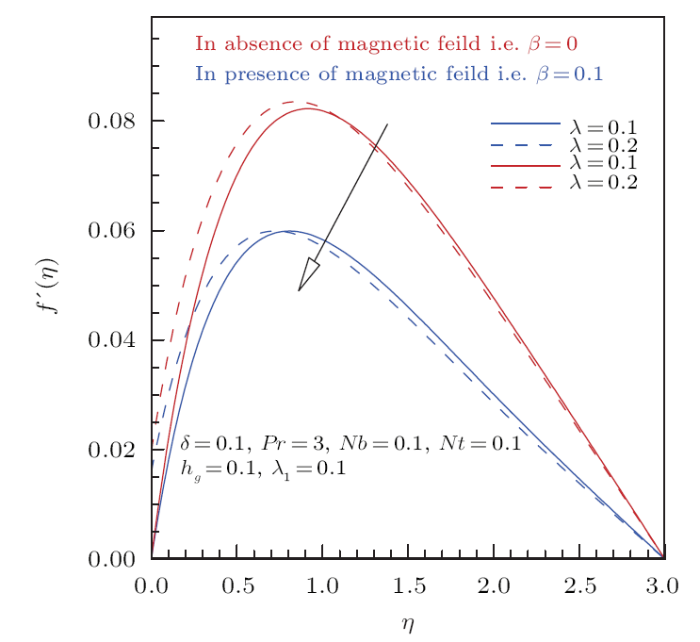
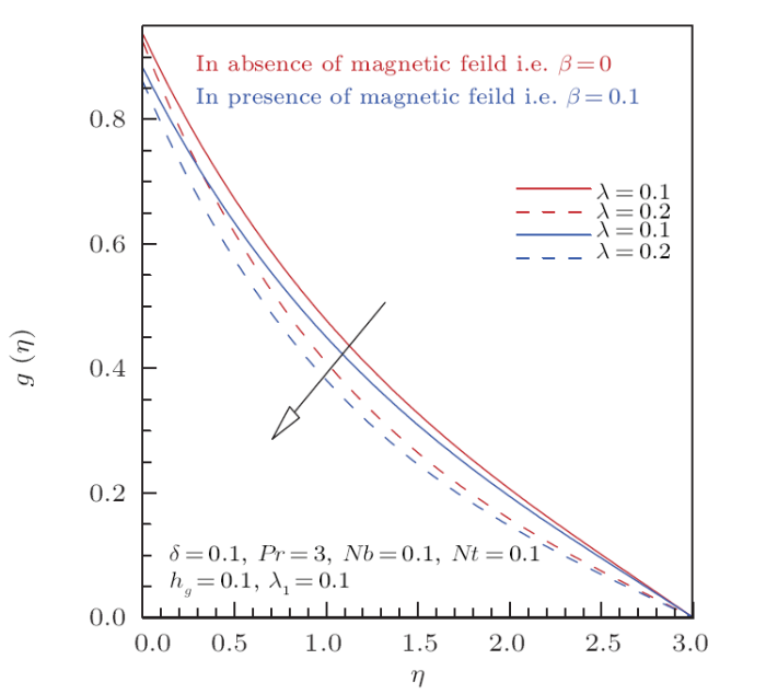
This section is enchanted to sketch the complete interpretation of sundry variables on flow, temperature and nano particle concentration profiles. To get thorough intellect about the present analysis Runge-Kutta method is implemented and to produce highly accurate results the coefficients of RK- method is improved by Cash and Carp scheme. Figures2 and 3 are adorned to check out the behavior of velocity slip parameter $\lambda$ on $f'(\eta)$ and $g(\eta)$ in the presence and absence of magnetic field $\beta$. Firstly, Fig.2 is plotted to analyze the behavior of momentum slip parameter $\lambda$ on radial velocity component for magnetic and non-magnetic cases. From the displayed sketch it is manifested that velocity field curves show diminishing magnitude with respect to incrementing values of momentum slip parameter $\lambda$ in the presence of magnetic field $\beta\neq0$ and in absence of magnetic field $\beta=0$. The reason behind this delineating aspect is that the radial velocity is persuaded by the rotational force. It is observed that the radial velocity diminishes thus the location of the maximum velocity shifts towards the rotated wall as momentum slip parameter $\lambda$ upsurges. It is also witnessed from these curves that without magnetic field momentum profile exhibits a significant increase as compared to the curves attained for magnetic field consideration. This is because the magnetic field is resistive force in nature that is why flow profile increases in absence of magnetic field and decreases in the presence of magnetic field. The attribute of tangential velocity curves for various values of momentum slip parameter $\lambda$ is plotted in Fig.3. This sketch examines decreased manner in $g(\eta)$ for mounting values of slip parameter $\lambda$. Physically, when momentum slip aspects $\lambda$ come into action the partial part of the fluid moves towards the non-azimuthal direction as an outcome $g(\eta)$ shows decrementing manner. Furthermore it also evident from this graph that magnetic field has same qualitatively effect on tangential velocity as $\lambda$ does on radial velocity, i.e.strong Lorentz force opposed the fluid motion.

Fig.2

New window|Download| PPT slide
Fig.2Effect of momentum slip parameter and magnetic parameter on $f'(\eta)$.

Fig.3

New window|Download| PPT slide
Fig.3Effect of momentum slip and magnetic parameter on $g(\eta)$.



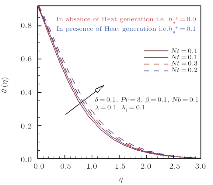
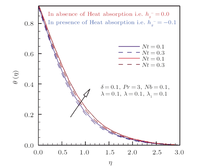
Figures 4 and 5 are drawn to evaluate the graphical aspects of thermophoretic parameter $Nt$ on thermal distribution $\theta(\eta)$ under the influence of heat generation/absorption parameter. It is obvious from Figs.4 and 5 that the thermal field of fluid flow mounts by intensifying the magnitude of heat generation in comparison to the variation in heat absorption coefficient. The fact is revealed due to the reason that by uplifting the magnitude of heat generation coefficient the thermal energy of the system raises and hence temperature of fluid flow enriches. Figures4 and 5 assess the physical significance of thermophoresis parameter $Nt$ on fluid temperature.

Fig.4

New window|Download| PPT slide
Fig.4Effect of thermophoresis parameter and heat generation parameter on $\theta(\eta)$.

Fig.5

New window|Download| PPT slide
Fig.5Effect of thermophoresis and heat absorption parameter on $\theta(\eta)$.



Figure 4 is depicted to analyze the behavior of temperature curve against the inciting values of $Nt$ in the presence and absence of heat generation parameter $h_{g}^{+}$. It is seen from these curves that the thermophoresis parameter $Nt$ is responsible for the increase of temperature and also corresponding boundary layer thickness. The reason behind that, thermophoresis is a force, which pushes the nano particle from higher temperature region to lower temperature region. Therefore higher values of thermophoresis parameter $Nt$ correspond to the strong thermophoretic force due to which movement of particle from hotter to colder region increases significantly. As a result fluid temperature enhances for positive values of thermophoresis parameter. Furthermore it is also divulged from the profile that temperature of fluid flow rises for heat generation $h_{g}^{+}$ parameter as compared to the absence of heat generation parameter. In Fig.5 the behavior of thermal distribution with respect to thermophoresis parameter and heat absorption parameter $h_{g}^{-}$ is interpreted. Similar behavior against $Nt$ is observed in temperature is observed. But in Fig.5 thermal distribution enriches in the absence of heat absorption parameter $h_{g}^{+}$ as compared to the presence of $h_{g}^{-}$.

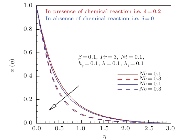
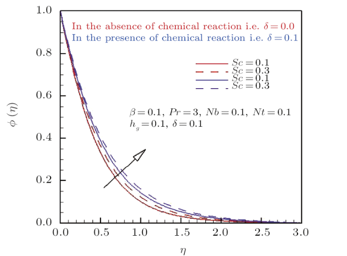
Profiles of non-dimensional concentration profiles are plotted in Figs.6 and 7 for altering magnitude of Brownian motion parameter and Schmidth number in the absence/attendance of chemical reaction. From these curves in Fig.6 it is depicted that nanoparticle concentration and respective solutal boundary layer thickness shows an consequence trend against positive values of $Nb$. It is seen that higher values of $Nb$ drops the nanoparticle concentration because increment in $Nb$ is responsible for random motion of nanoparticle as a consequence concentration boundary layer thickness decreases which results decrease in concentration profile. While Fig.7 displays the impact of Schmidth number on nano particle concentration profile. One can see that Schmidth number decline the volumetric fraction of nanoparticle massively. Mathematically Schmidth number is the ratio of thermal to mass diffusion, therefore inciting values of Schmidth number moderates mass diffusivity and hence concentration of nanoparticles. As for the physical significance of constructive chemical reaction on nanoparticle concentration profile is identically same in both figures. Both of these figures display the concentration profile across the flow domain and it is evident that existence of constructive chemical reaction increases the concentration profile resulting thicker concentration boundary layer. Trends with the aid of numerical data disclosed in Tables 2 and 3 with respect to magnetic parameter $\beta$, momentum slip parameter $\lambda$, thermophoresis parameter $Nt$, Schmidth number $Sc$ and Prandtl number $Pr$ on Nusselt number $(Re_{\bar{r}})^{-1/2}Nu$ are elucidated. From the attained data it is found that by intensifying the magnitude of magnetic parameter $\beta$, Schmidth number $Sc$ and Prandtl number $Pr$ there is uplift in values of heat transfer coefficient whereas diminishing attribute is observed against up surging values of momentum slip parameter $\lambda$, thermophoresis parameter $Nt$ and Brownian motion parameter $Nb$. The mounting behavior of Nusselt number $(Re_{\bar{r}})^{-1/2}Nu$ with respect to $\beta$, $Sc$, and $Pr$ can be justified by the fact that all of these parameters produces resistive force in the flow field. So this productivity of resistance among fluid molecules raises the temperature of the fluid flow and hence the coefficient of convective heat transfer enriches. Furthermore these results are compared with the previous literature published by Hayat et al.^[19] It is found from the comparison that results are total covenant to each other. Numerical variation in $(Re_{\bar{r}})^{-1/2}Sh$ is disclosed in Tables 2 and 3 with respect to magnetic parameter $\beta$, momentum slip parameter $\lambda$, thermophoresis parameter $Nt$, Schmidth number $Sc$ and Prandtl number $Pr$ is manipulated. From the calculated values it is found that by increasing $Nt$, $Sc$, $Pr$, and $Nb$ mass flux coefficient enhances. But reverse pattern is found for incrementing values of $\beta$ and $\lambda$. The intensifying magnitude of mass flux coefficient with respect to $Nt$, $Sc$, $Pr$, and $Nb$ is due to the reason that all of these mentioned factors decease the motion of fluid molecules and hence the concentration profile boosts. Furthermore these results are also compared to check the assurance of present computed results by making excellent matching with finding provided by Hayat et al.^[19]

Fig.6

New window|Download| PPT slide
Fig.6Effect of Brownian motion parameter and chemical reaction parameter on $\phi(\eta)$.

Fig.7

New window|Download| PPT slide
Fig.7Effect of Schmidth number and chemical reaction parameter on $\phi(\eta)$.



Tab.2


Tab.2Comparison and Variation for Nusselt number w.r.t above mentioned parameters.

New window|CSV

Tab.3


Tab.3Comparison and Variation for Nusselt number w.r.t above mentioned parameters.

New window|CSV

Tab.4


Tab.4Comparison and Variation in Sherwood number w.r.t above mentioned parameters.

New window|CSV

Tab.5


Tab.5Comparison and Variation in Sherwood number w.r.t above mentioned parameters.

New window|CSV

5 Closing Remarks

The viscid nanoliquid flow due to rotational rigid disk is considered along with some other physical effects. The obtained observations are itemized as follows:

(i) The application of magnetic field brings decline in fluid velocity.

(ii) Tangential velocity is diminishing function of velocity slip parameter.

(iii) Temperature profile reflects higher values via heat generative parameter while opposite trends are perceived towards heat absorption parameter.

(iv) Nanoparticle concentration admits same variations towards both Brownian motion and Schmidth number.

Acknowledgment

The authors would like to express their gratitude to King Khalid University, Abha 61413, Saudi Arabia, for providing administrative and technical support.

Reference View Option By original order
By published year
By cited within times
By Impact factor

[1] T. V. Karman , Z. Angew. Math. Mech. 1( 1921) 233.
[Cited within: 1]

[2] M. Turkyilmazoglu and P. Senel , Int. J. Thermal Sci. 63 ( 2013) 146.
[Cited within: 1]

[3] G. S. Guram and M. Anwar , Z. Angew. Math. Mech. 61 ( 1981) 589.
[Cited within: 1]

[4] M. M. Rashidi, N. Kavyani, S. Abelman , Int. J. Heat Mass Transfer. 70 ( 2014) 892.
[Cited within: 1]

[5] M. Turkyilmazoglu, Comput. Fluids 94 ( 2014) 139.
[Cited within: 1]

[6] M. Mustafa, J. A. Khan, T. Hayat, A. Alsaedi, J. Mol. Liq.211 ( 2015) 119.
[Cited within: 1]

[7] M. Sheikholeslami, M. Hatami, D. D. Ganji, J. Mol. Liq.211 ( 2015) 577.
[Cited within: 1]

[8] S. U. Choi, ASME Publications Fed.231 ( 1995) 99.
[Cited within: 1]

[9] J. Buongiorno, J. Heat Transfer.128 ( 2006) 240.
[Cited within: 1]

[10] H. Chen, S. Witharana, Y. Jin , et al. Particuology 30( 2009) 151.
[Cited within: 1]

[11] S. Nadeem and C. Lee, Nanoscale Res. Lett.1 ( 2012) 94.
[Cited within: 1]

[12] S. M. Peyghambarzadeh, S. H. Hashemabadi, M. S. Jamnani, S. M. Hoseini, Appl. Ther. Eng.31 ( 2011) 1833.
[Cited within: 1]

[13] H. Alfven , Nature(London) 150 ( 1942) 405.
[Cited within: 1]

[14] T. Sarpkaya, AIChE J.7 ( 1961) 324.
[Cited within: 1]

[15] S. J. Liao, J. Fluid Mechanics 488 ( 2003) 189.
[Cited within: 1]

[16] F. Mabood, W. A. Khan, A. M. Ismail, Chem. Eng. J.273 ( 2015) 430.
[Cited within: 1]

[17] M. Y. Malik, T. Salahuddin, A. Hussain, S. Bilal , J. Magn. Magn. Mater. 395 ( 2015) 271.
[Cited within: 1]

[18] N. S. Akbar, A. Ebaid, Z. H. Khan , J. Magn. Magn. Mater. 382 ( 2015) 355.
[Cited within: 1]

[19] T. Hayat, T. Muhammad, S. Ali , Comput. Methods Appl. Mech. Eng. 315 ( 2017) 467.
[Cited within: 3]

[20] B. J. Gireesha, M. Archana, B. C. Prasannakumara , et al. Int. J. Numer. Meth. Heat Fluid Flow 27 ( 2017) 2858.
[Cited within: 1]

[21] M. Archana, B. J. Gireesha, B. C. Prasannakumar, R. S. R. Gorla , Multidiscipl. Model. Mater. Struct. 13 ( 2017) 628.
[Cited within: 1]

[22] B. J. Gireesha and N. G. Rudraswamy , Int. J. Engg. Sci. Tech. 6 ( 2014) 13.
[Cited within: 1]

[23] K. G. Kumar, R. U. Haq, N. G. Rudraswamy, B. J. Gireesha, Results Phys.7 ( 2017) 3465.
[Cited within: 1]

[24] M. Archana, B. J. Gareesha, P. Venkatesh, et al. J. Nanofluids 6 ( 2017) 232.
[Cited within: 1]