摘要:声镊一般是指利用声辐射力原理对微小粒子进行悬浮和移动的一种技术. 粒子的水平移动是声镊操控粒子的常见方式之一. 本文理论推导了声辐射力与声压之间的直接关系, 结果表明声压极大值点(聚焦点)与声辐射力势能的极小值点之间具有对应关系, 并根据声阵列相位合成原理建立了声镊声场聚焦模型. 文章基于数值仿真方法, 以双侧16阵元声镊装置为例, 分析了粒子水平移动的控制方法和稳定性. 由于受到重力影响, 粒子水平移动过程中必须考虑竖直方向的平衡问题. 声场中, 不同位置的粒子向各方向水平移动的稳定性是不同的. 越靠近阵列中心, 粒子移动的稳定性越高. 粒子移动步长(精度)对移动稳定性也有重要影响. 一般来说, 步长越短稳定性越高. 本模型中, 移动步长减小1/2, 稳定性提了高近40%. 研究结果对于设计声镊粒子移动控制方法, 规划粒子移动路径, 推动声镊技术应用等具有理论意义.
关键词: 声镊/
粒子操控/
相位调控/
声辐射力

English Abstract

全文HTML

--> --> -->

声镊技术属于无接触式操控技术的一种, 是近年来声学领域的热点研究方向之一. 从原理上来说, 声镊技术主要是利用声辐射力效应使微小颗粒被束缚在势能极小值的位置处, 进而通过调控该汇聚点的位置实现对微粒的操控. 相比其他类型的无接触式操控方法, 声镊技术具有独特的优势. 不同于磁悬浮和光镊等技术, 声镊技术不需要悬浮微粒具有铁磁性^[1]或透光性^[2]等特殊性质. 在声镊设计过程中仅需考虑微粒的密度和体积等基本参数即可. 声镊技术很少产热, 对微粒本身基本没有有害的影响^[3]. 除此之外, 声镊装置的安全性较高, 成本也较低, 同等能量输入的条件下, 声镊装置产出的能量要远远高于光镊装置. 声镊装置悬浮的最大微粒直径可以达到厘米量级^[4], 而光镊操控的最大微粒直径仅在微米量级^[5]. 这些独有优势是声镊在近年来成为热点研究的原因.
声镊技术起源于声悬浮技术, 是声辐射力原理的应用方向之一^[6]. 1990年, Wu^[7]基于单超声换能器装置首次实现了青蛙卵的悬浮与移动, 由此提出了声镊的概念. 因此从技术组成来讲, 声镊技术可以分为悬浮和移动两个部分. 一般来说, 声镊装置首先将微粒进行悬浮, 而后通过移动技术可以将微粒搬运到目标位置. 声悬浮技术主要包括驻波场^[8]、行波场^[9]和声流^[10]等基本机理. 通过增加声透镜装置, 还可形成涡旋声场和瓶声场等多种特殊的声悬浮声场形式^[11]. 微粒移动技术是声镊装置的关键技术之一, 也是其有别于声悬浮装置的关键点. 大体上来说, 可包括装置移动技术和参数调节技术两种. 所谓装置移动技术, 是通过将声悬浮装置与步进电机相结合, 通过控制步进电机实现声悬浮装置的整体移动, 进而实现悬浮微粒的移动. 参数调节技术主要是通过调节换能器的幅值和相位等基本参数, 实现微粒在声镊装置内部的位置移动.
以驻波场声镊为例, 该装置通常由一对上下正对放置的平面阵列组成. 此时, 可以改变其中某些阵元输出信号的幅值^[12], 也可以改变其中某些阵元输出信号的相位^[13], 或者同时改变幅值与相位分布^[14,15,16]均可以实现微粒水平或竖直移动的目的. 在幅值调节技术中, 通过调节相邻两个换能器之间的声信号幅值差改变势能极小值点的位置, 从而实现微粒的移动. 但此时微粒仅能沿着相邻换能器的中心点连线移动, 而不能沿着其他方向移动, 限制了声镊装置微粒操控的有效范围. 相位调控技术具有精度高、有效范围广等优势, 也是目前多种声镊装置采用的技术途径. 但是目前关于相位调节方法的适用范围和有效精度等问题的研究还非常有限. 本文基于相位合成原理和声辐射力理论建立了换能器阵列相位控制模型, 分析了重力对微粒平衡位置的影响. 基于有限元方法模拟了换能器阵列相位调控方法, 分析了相位调控精度对微粒移动方向和有效操控范围的影响. 本文研究结果对微粒移动路径规划以及设计高精度声镊装置等具有理论意义.

由于微粒总是在势能最小的位置处达到平衡状态, 所以, 势能最小值(极小值)点处可供微粒悬浮, 移动该点又可以使微粒跟随移动, 达到操控的目的. 基于此, 构建与移动势能最小值(极小值)点就成了变相位声镊发挥作用的关键步骤.
根据Gor’Kov^[17]的声辐射力势能理论, 微粒受到的声辐射力可以表达为

$ \mathit{F}=-\nabla U, $

$ U=2\mathrm{\pi }{R}^{3}\left(\frac{{p}_{\mathrm{r}\mathrm{m}\mathrm{s}}^{2}}{3{\rho }_{0}{c}_{0}^{2}}-\frac{{\rho }_{0}{v}_{\mathrm{r}\mathrm{m}\mathrm{s}}^{2}}{2}\right), $

其中, F为微粒受到的声辐射力, $ U $为声辐射力势能, R为微粒半径, $ {\rho }_{0} $为介质密度, $ {c}_{0} $为室温下的声速, ${p}_{\mathrm{r}\mathrm{m}\mathrm{s}}$和$ {v}_{\mathrm{r}\mathrm{m}\mathrm{s}} $分别为均方根声压和均方根质点振速. 在Gor’Kov^[17]提出的理论中, 声辐射力势能是声压和质点振速的多值函数, 如果能够将声辐射力势能变成声压或者质点振速的单值函数则会使声辐射力势能变得直观易处理. 在传播过程中, 小振幅声波的波形畸变会累积产生非线性效应, 如果传播的距离不是很远(定义马赫数$ {M}_{a} $为质点速度和声速之比, 当$ {M}_{a}\ll 1 $时, 非线性效应可以忽略), 仍然可以用线性声场^[18,19]. 这里将质点振速用局部声压来表示. 线性声学中有

$ \mathit{v}=-\frac{1}{{\rho }_{0}}\int \nabla p\mathrm{d}t. $

将换能器视为活塞声源, 假设活塞以速度$u= $$ {u}_{a}{\mathrm{e}}^{\mathrm{j}\omega t}$振动, 其向半空间辐射的声压场可以表示为^[20]

$ p\left(\theta ,r\right)=\mathrm{j}\omega \frac{{\rho }_{0}{u}_{a}{a}^{2}}{2r}\left[\frac{2{\mathrm{J}}_{1}\left(ka\mathrm{sin}\theta \right)}{ka\mathrm{sin}\theta }\right]{\mathrm{e}}^{\mathrm{j}\left(\omega t-kr\right)}, $

其中$ \mathrm{j} $为虚数单位, $ \omega $为角频率, $ k $为波数, $ {\rho }_{0} $为媒质密度, $ {u}_{a} $为换能器表面振速幅值, $ a $为换能器表面半径, $ r $为换能器表面中心到目标点的距离, $ \theta $为矢径$\boldsymbol{r}$与换能器表面法向矢量的夹角, $ t $是时间, ${\mathrm{J}}_{1}\left(\cdot \right)$是一阶贝塞尔函数. 这里省略声压的虚部. 将(4)式代入(3)式得

$ v=\frac{\mathrm{j}kr+1}{\mathrm{j}\omega \rho r}p. $

将(5)式代入(2)式:

$ U=2\mathrm{\pi }{R}^{3}\cdot \varGamma \cdot {p}^{2},\;\varGamma =\frac{-{k}^{2}{r}^{2}+3}{6{\rho }_{0}{k}^{2}{r}^{2}{c}_{0}^{2}}.$

当$r > \dfrac{\sqrt{3}}{k}$时, $\varGamma < 0$. 由于超声场中$\dfrac{\sqrt{3}}{k}~2\times {10}^{-3}\;\mathrm{m}$, 因而在实验中基本可以将$ \varGamma $视为负数. 所以声压$ p $的极(最)大值点即为声辐射力势能$ U $的极(最)小值点. 通常, 可利用聚焦声场获得局部声压的极大值. 图1给出了换能器与焦点之间的几何关系.
图 1 换能器与焦点之间的几何关系. 坐标原点位于下方阵列的中心处, x轴和y轴分别平行于方形阵列的两个边. 这里将换能器与聚焦点之间的距离视为换能器表面中心与聚焦点之间的距离, z轴垂直指向上方阵列. 图中, 某换能器中心到聚焦点在该阵元平面上的投影点之间的距离为$ d $, 上下阵列平面之间的距离为H, 换能器与聚焦点间的距离为$ r $, $ d $与$ r $之间所夹锐角记为$ \xi $
Figure1. Geometric relationship between the transducer and the focal point. Origin of the coordinate is located at the center of the lower array, and the x-axis and y-axis are parallel to the two sides of the square array. Here, the distance between the transducer and the focus point is regarded as the distance between the center of the transducer surface and the focusing point, and the z-axis points vertically to the upper array. In the figure, the distance between the center of a certain transducer and the projection point of the focal point on the array plane is $ d $, the distance between the upper and lower array planes is H, and the distance between the transducer and the focal point is $ r $. The acute angle in between $ d $ and $ r $ is recorded as $ \xi $

由于声压中含有时空周期变化的指数项, 所以可以运用相位调制的方法, 使声压聚焦于目标点. 假设上下两个阵列相距$ H $, 聚焦点到上方阵列的距离为$ {H}_{1} $, 到下方阵列的距离为$ {H}_{2} $, 坐标原点位于下方阵列的中心处, x轴和y轴分别平行于方形阵列的两个边, z轴垂直指向上方阵列. 聚焦点位于两个平面阵列中间的任意一个位置$ \left({x}_{0}, {y}_{0}, {H}_{2}\right) $处. 将聚焦点到任意1个阵元的距离$ r $视为聚焦点到该换能器表面中心点的距离, 聚焦点到平面上的投影与换能器表面中心之间的距离为$ d $, $ d $与$ r $之间所夹锐角记为$ \xi $. 将问题一般化, 上下平面总共有2N个阵元, 对应的$ r $值和$ \xi $值也有2N个. 下表面的某个阵元表面中心点的坐标为$ \left({x}_{1}, {y}_{1}\right) $, 那么其到聚焦点的投影点的距离$ \mathrm{为} $

$ {d}_{0}=\sqrt{{\left({x}_{0}-{x}_{1}\right)}^{2}+{\left({y}_{0}-{y}_{1}\right)}^{2}}.$

该阵元所对应的变量:

$ r=\sqrt{{H}_{2}^{2}+{d}_{0}^{2}}, $

$ \xi =\mathrm{a}\mathrm{r}\mathrm{c}\mathrm{t}\mathrm{a}\mathrm{n}({{H}_{2}}/{{d}_{0}}), $

每个换能器在聚焦点处的声压贡献量为

$ {p}_{n}={A}_{n}{\mathrm{e}}^{-\mathrm{j}k{r}_{n}},n=1,2,3,\cdots ,2N. $

$ {A}_{n}=\mathrm{j}\omega \frac{{\rho }_{0}{u}_{a}{a}^{2}}{2{r}_{n}}\left[\frac{2{\mathrm{J}}_{1}\left(ka\mathrm{sin}\theta \right)}{ka\mathrm{sin}\theta }\right]{\mathrm{e}}^{\mathrm{j}\omega t}, $

其中$\theta =\dfrac{\pi }{2}-\xi$. 聚焦点处的总声压为

$ {p}_{t}=\sum _{n=1}^{2N}{p}_{n} $

为了使同一点处的声压达到最大, 在换能器的激励信号上引入迟滞相角$ {\varphi }_{n} $. 此时聚焦点处的声压强度为

$ {p}_{t}=\sum _{i=1}^{2N}{A}_{n}{\mathrm{e}}^{\mathrm{j}\left({\varphi }_{n}-k{r}_{n}\right)}. $

记$ {\eta }_{n}={\varphi }_{n}-k{r}_{n} $, $ f\left(\eta \right)={\mathrm{e}}^{\mathrm{j}\eta } $为周期函数, 一个完整的周期内$ f $的最大值为1. 不妨认为此时$ \eta $为0, $ {A}_{n} > 0 $, 所以$ {p}_{t} $此时取得最大值, 迟滞相角$ {\varphi }_{n}=k{r}_{n} $, 这样就可以实现声压在目标点处的聚焦. 目标点处形成的声压极大值同时也是声辐射力势能的极小值, 微粒在仅受声辐射力作用的情况下将被束缚于目标点. 聚焦点的移动, 实质上就是声压在不同点处实现聚焦. 不同的点到达各换能器距离不一, 而距离又决定了相角的大小, 所以引入的迟滞相角也不一致. 这样当聚焦点的位置在两点之间变换时, 根据不同的点改变各换能器发射信号的相角即可.
平面移动是声镊的典型操作之一, 本文主要讨论粒子在平面上移动的情况. 微粒从某一位置移动至下一个位置的过程中系统发生的变化包括: 极小势能点的移动和微粒的受力移动. 该过程如图2(a)—(c)所示. 当形成声压聚焦点时, 微粒被束缚于该聚焦点处, 即势能极小值点处. 通过改变各换能器发射信号的相角, 从而在平面内改变聚焦点的位置, 即实现了势能极小值点的移动. 由于聚焦点的移动, 微粒暂时地移动到力的汇聚区的边缘, 在不脱离力的汇聚区范围的情况下, 微粒受到1个指向势能极小值点的力的作用, 在没有水平方向外力干扰的情况下, 微粒最终会运动至聚焦点处.
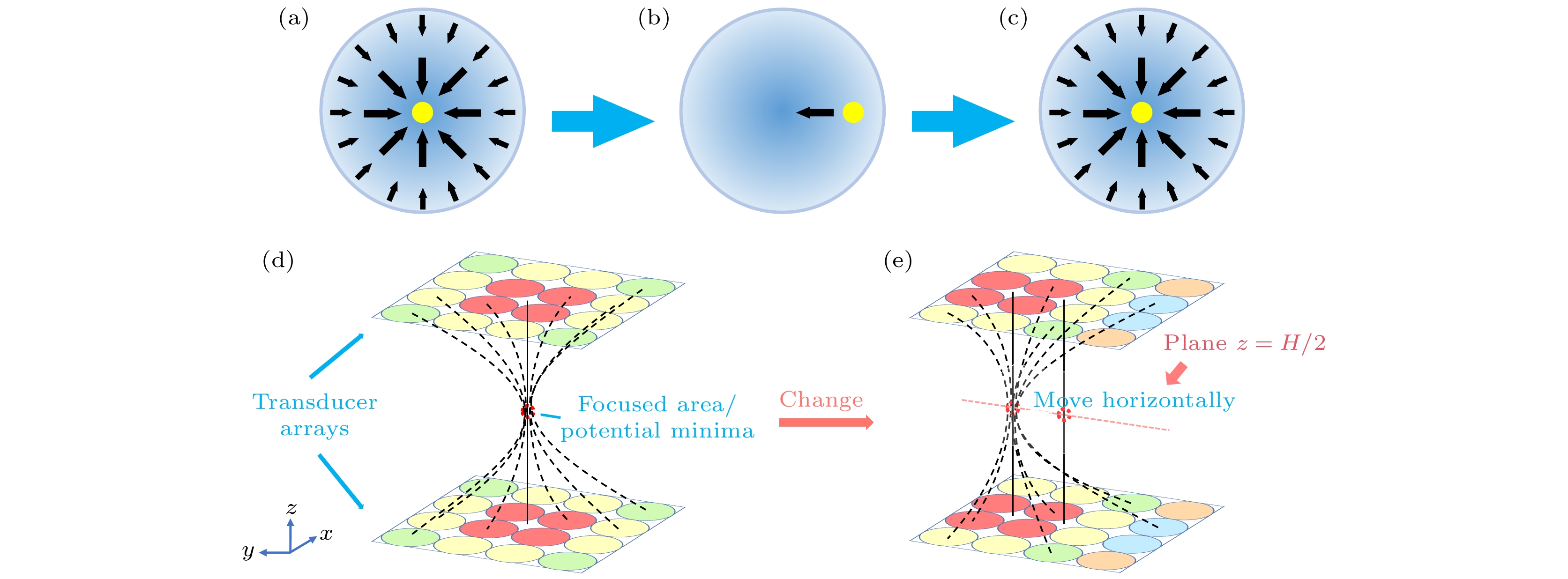图 2 (a)?(c)微粒在平面内移动过程的俯视示意图, 其中(a)微粒被束缚在聚焦点处, 黑色箭头代表力的分布; (b)聚焦点移动后微粒与力的汇聚区相对位置示意图, 黑色箭头代表微粒所受力的方向; (c)微粒回到聚焦点; (d), (e)力的汇聚区移动的示意图. 上下两块正对的正方形区域为换能器阵列所在平面, 上嵌的圆圈代表换能器, 不同颜色代表不同的相位. 力的汇聚区以红色虚线圆圈表示, 黑色虚线簇代表声线, 黑色实线为辅助线, 用以标明力的汇聚区位置, 粉色虚线为力的汇聚区移动轨迹所在直线
Figure2. (a)?(c) Schematic top views of the movement of particles in a plane: (a) Particles are bounded at the focus point, and the black arrow represents the distribution of acoustic radiation force (ARF); (b) schematic diagram of the relative position of the particle and the convergent area of the force after the focus point moves, with a black arrow representing the direction of the force acting on the particle; (c) particle returning to the focus point. (d), (e) Schematic diagrams of the movement of the force convergence area. The upper and lower two square areas facing each other are the planes where the transducers are located. The circles embedded on the planes represent the transducers, and different colors represent different phases. The force convergence area is represented by a red dashed circle. The black clusters of dashed lines represent acoustic rays. The black solid line is an auxiliary line to indicate the location of the force convergence area, and the pink dashed line is the straight line where the trajectory lies.

以图2(d)和图2(e)中描述的过程来说明具体的移动方法. 当实现如图2(d)所示聚焦时, 换能器相位分布情况为: ${\varphi }_{\mathrm{红}}=k{r}_{\mathrm{红}}=13.593\;\mathrm{r}\mathrm{a}\mathrm{d}, {\varphi }_{\mathrm{黄}}=k{r}_{\mathrm{黄}}= $$ 17.092\;\mathrm{r}\mathrm{a}\mathrm{d}, {\varphi }_{\mathrm{绿}}=k{r}_{\mathrm{绿}}=19.988\;\mathrm{r}\mathrm{a}\mathrm{d};$当聚焦点需要变换至图2(e)所示位置时, 换能器相位相应地变化为: ${\varphi }_{\mathrm{红}}=k{r}_{\mathrm{红}}=13.593\; {\rm{rad}}, {\varphi }_{\mathrm{黄}}=k{r}_{\mathrm{黄}}=17.092\;\mathrm{r}\mathrm{a}\mathrm{d},$${\varphi }_{\mathrm{绿}}\;=\;k{r}_{\mathrm{绿}}\;=\;19.988\;\mathrm{r}\mathrm{a}\mathrm{d},\; {\varphi }_{\mathrm{蓝}}\;=\;k{r}_{\mathrm{蓝}}=22.514\;\mathrm{r}\mathrm{a}\mathrm{d}, \;$$ {\varphi }_{\mathrm{橙}}=k{r}_{\mathrm{橙}}=24.785\;\mathrm{r}\mathrm{a}\mathrm{d}. $
将操控面选定为平面z = H/2, 如图2(e)所示. 驻波场中声辐射力沿轴向的分布如图3所示, 声辐射力和声压一样沿着图中的z轴周期变化, 正负代表其方向, 最大值介于两个最小值之间. 不考虑重力的影响时, 粒子悬浮于声辐射力为0的汇聚点处. 但由于微粒自身重力不可忽略, 对于悬浮会产生一定的影响. 若能够悬浮, 粒子位置将在力的汇聚零点之下, 相邻的力的最大值之上^[21], 即图3中红色虚线之间的区域. 当声压为一简谐波时, 声辐射力的波长为声压波长的一半, 所以声辐射力极值和相邻的声辐射力零值相距${\lambda }/{8}$^[22], 这里$ \lambda $指声压的波长. 本文中微粒稳定悬浮的高度位于${H}/{2}-{\lambda }/{8}$和${H}/{2}$之间. 除了垂直正对的换能器之间会产生驻波外, 其余换能器之间也会产生驻波点, 那么声辐射力的最大值和最小值可能不在理论位置. 因此, 微粒的移动并不能稳定在某一个确定的高度, 而是在z = H/2附近. 在第3节中会详细讨论该问题.
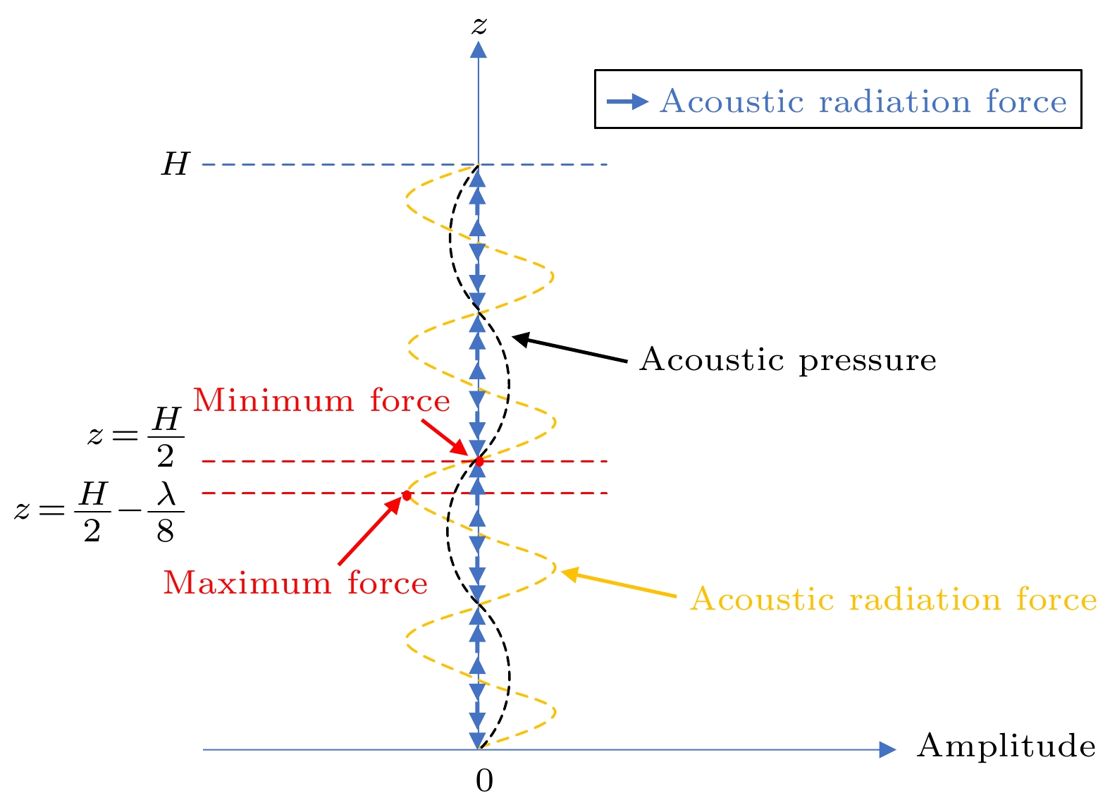图 3 某对换能器在垂直方向产生的驻波声场中的相关元素示意图. 黑色虚线为声压的垂向分布, 黄色虚线为声辐射力的垂向分布, 蓝色箭头的长短和方向代表声辐射力的大小和方向. z轴上的H/2高度处应为力的汇聚点, 其下方1/8个波长处应为相邻的1个力的极大值对应的高度
Figure3. Schematic diagram of the relevant elements in the standing wave acoustic field generated by a pair of transducers in the vertical direction. The black dashed line is the vertical distribution of acoustic pressure, the yellow dashed line is the vertical distribution of the ARF. The length and direction of the blue arrow represent the magnitude and direction of the ARF. The height of H/2 on the z axis should be the convergence point of the force, and the one-eighth of the wavelength below it should be the height corresponding to the adjacent maximum force.

结合具体例子给出计算和分析的过程, 模型结构简图见图1. 上下两个阵列平面各由16 (4 × 4)个换能器组成, 正对放置, 阵元之间紧密排列. 每个换能器直径为1 cm, 发射的声波频率为40 kHz, 在室温(25 ℃)下波长$ \lambda $为8.575 mm. 上下两个阵列平面相距4个波长. 阵元的仿真以实验室现有的换能器为例, 测得其正常工作时距离表面1.2 cm处的声压约为141 Pa. 此时, $ {M}_{a}=0.004\ll 1 $, 可以使用线性声学的理论. 利用Gor’Kov的理论((1)式和(2)式), 在有限元仿真软件(COMSOL Multiphysics)中可以计算出域上的势能分布. 三维模型参数如图1所示, 研究类型选取为 “压力声学-频域”. 换能器区域设为平面波辐射边界, 上下正对的两换能器相位一致, 所有换能器的幅值相同. 网格剖分设为自由四面体网格, 最大单元边长为1.4 mm, 符合声学有限元计算条件. Gor’Kov的理论应用的前提条件是$ a\ll \lambda $, 即微粒的半径远小于入射波波长. 这个条件引入的目的是确保微粒内部的声共振模式难以被激发, 将微粒视为刚性的而忽略压缩性^[18]. 计算时选取的悬浮对象是半径为1 mm的粒子. 由聚焦而形成的势能低值区(图4(c)和图4(d)中的亮斑)有许多指代方法, 如声压聚焦区、力的汇聚区、势能低值区等, 在后面的内容中统一称为力的汇聚区.
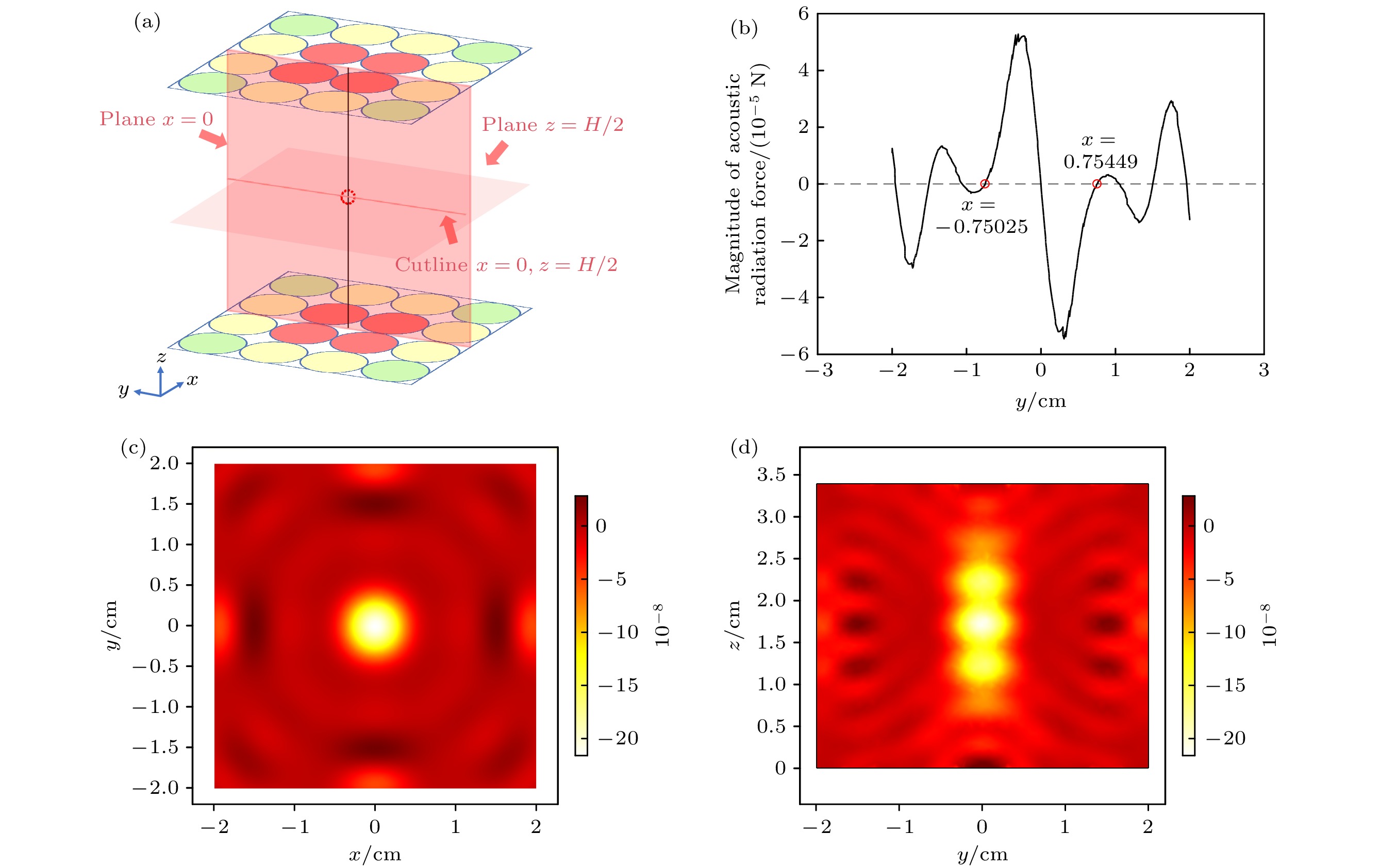图 4 聚焦点在中心时声辐射力势能的分布　(a)聚焦点在中心时的相位分布示意以及截面z = H/2、截面x = 0、截线x = 0、截线z = H/2所在位置; (b)截线x = 0, z = H/2上声辐射力在y方向的分量; (c)平面z = H/2上的声辐射力势能的分布; (d)平面x = 0上的声辐射力势能分布
Figure4. Distribution of ARF potential energy when the focal point is at the center: (a) Phase distribution diagram when the focal point is at the center and the position of section z = H/2, section x = 0 and section line x = 0, z = H/2; (b) component of the ARF in the y direction on the section line x = 0, z = H/2; (c) distribution of ARF potential energy on the plane z = H/2; (d) distribution of ARF potential energy on the plane x = 0.

由于微粒的移动和力的汇聚区移动相关, 汇聚区的移动特性将关系到微粒移动的稳定性. 对于平面内点到点的移动, 不失一般性地将其视为在二维网格点上的移动. 为了简单起见, 选择正交格点. 格点间距的选择和声辐射力的分布密切相关. 在操控面上, 从过聚焦点的一条截线上看声辐射力分布, 声辐射力围绕焦点形成1个圆形汇聚区, 从中心向外侧先增大后减小至0, 零值的位置即为该汇聚区域的边界. 图4(b)中的两点数据显示此时平面上的声辐射力的汇聚区半径约为0.89$ \lambda $(0.76 cm). 在正交格点中, 格对角线总是长于格边, 那么格对角线的距离最多为0.89$ \lambda $. 在这种情况下, 格点间距为0.63$ \lambda $(0.54 cm). 考虑适当缩小对角线距离, 使得在聚焦点沿格对角线移动时微粒依然位于汇聚区内, 所以将格点间距选为0.58$ \lambda $(0.5 cm), 如图5(a)中的橙色格线所示.
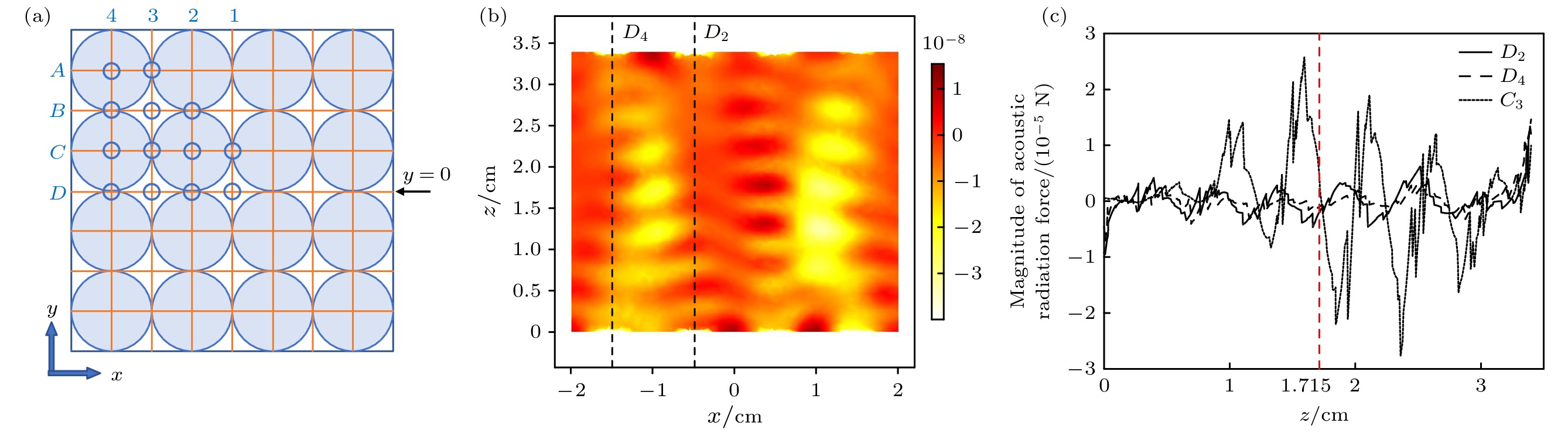图 5 (a)格点化操控表面以及部分聚焦位置. 根据对称性将所有点归类为图中的10个实线蓝圈所标出的点, 3个虚线蓝圈标出的点为补充遗漏路径需要绘制的点. 经线从中心向外围以递增数字1?4标注, 纬线自上而下以A, B, C, D标注. 这样任意一点可以以字母与数字的组合命名, 字母在前数字在后, 如中心处的点为D₁点. (b)聚焦点在C₃处时, y = 0截面上声辐射力势能的分布. 横坐标为x轴刻度, 纵坐标为z轴刻度. 图中标注出了D₂和D₄处的垂直截线. 当聚焦点位于C₃时, 取D₂, D₄, C₃这3个位置处的3条垂直截线, 绘制了沿其分布的垂向声辐射力于(c)图中, 正负代表方向, 红色虚线标注出高度z = 1.715 cm
Figure5. (a) Grid on the manipulation plane and part of the focus position. According to symmetry, all points are represented as the points marked by the 10 solid blue circles in the figure, and the points marked by the 3 dashed blue circles are the points that need to be drawn to supplement the missing path. Longitude lines are marked with increasing numbers 1?4 from the center to the periphery, and latitude lines are marked with A, B, C, and D from top to bottom. In this way, any point can be named with a combination of letters and numbers, with letters in the front and numbers in the back, for example, the point at the center is the D₁ point. (b) Distribution of the ARF potential energy on the y = 0 section when the focal point is at C₃. The coordinates of x axis and z axis are recorded on abscissa and ordinate respectively. The positions of D₂ and D₄ are marked in the figure. The distribution of vertical ARF along three vertical cutlines D₂, D₄, C₃ are depicted in panel (c) when focusing point is located at C₃. The signs of ARF represent their directions. Red dashed line marks the latitude of z = 1.715 cm.

此时, 格点化后的阵列表面共有49个点. 考虑到在边界处声压难以聚焦, 或者聚焦效率极低, 且微粒一旦移出边界便不可控, 所以边界处并未划分格点. 为了便于指代, 纬线自上而下以字母标注, 经线从右至左以数字标注, 指代时字母在前数字在后, 比如阵列中心处的点称为D₁点. 根据对称性, 将这些点归类为10个点, 相邻点之间的转移路径, 加上B₄到B₃, C₃到B₂以及D₂到C₁之间的3条特殊路径即可以囊括平面格点上所有的移动情形.
当力的汇聚区移动, 微粒能够跟随移动需要满足两个条件. 首先, 要将微粒稳定在操控平面附近; 其次, 微粒要位于汇聚区内. 对于第1点, 聚焦点移动后, 原位置处力的极小值点上下移动范围不能过大, 且原位置处减弱后的极大垂向声辐射力必须依然大于重力, 这样保证操控基本上位于水平面内. 对于第2点, 只有当原位置在焦点移动后依然位于汇聚区内, 微粒在平面内才可获得向中心移动的作用力, 否则该移动路径不稳定.
聚焦点可能位于10个点的任意一处, 而聚焦点所在的每一个位置都可以视为从该点周围的某一点移动而来. 遍历聚焦点的所有可能位置, 选取各位置处H/2高度附近的力的极小值点处所对应的平面和其下方相邻的一个力的极大值点处所对应的平面, 通过这些平面上水平力的分布情况判断周围的点是否包含在汇聚区内, 从而判断移动是否满足第2个条件. 按理想情况来看, 即势能场不发生变形, 极大值点和极小值点的位置都会相对固定, 分别位于${H}/{2}$和${H}/{2}- {\lambda }/{8}$高度附近. 但在聚焦点靠近边界的过程中, 不仅力的汇聚区的形状会发生变化, 力的汇聚区的位置也会发生横向与纵向的偏移, 从而导致当聚焦点在某些位置时其周围点上力的分布发生巨大的变化, 使得移动变得极不稳定. 理论上来讲, 当聚焦点位于操控平面上的某一格点处时, 该点和周围点上的垂向声辐射力应均为极小力, 即${H}/{2}=1.715\;\mathrm{c}\mathrm{m}$应为力的极小值所在高度. 但是当边缘附近声场形态发生改变时, 力的极小值所在高度定会发生改变. 规定当聚焦点和周围点力的极小值位于高度${H}/{2}- {\lambda }/{8}=1.608\;\mathrm{c}\mathrm{m}$之上且高度${H}/{2}+ {\lambda }/{8}=1.822\;\mathrm{c}\mathrm{m}$之下时, 视操控为稳定操控, 超出该范围即为不稳定操控.
以C₃点为例, 图5(b)给出了当聚焦点在C₃位置处时$ y=0 $截面上声辐射力势能的分布. 可以看出, 相比于在聚焦中心C₃处的声辐射力分布, D₂和D₄处声辐射力的分布发生了明显的改变, D₂和D₄处力的相位发生明显偏移, D₄处周期性明显减弱, 见图5(c)中3条曲线的对比. 这样, 微粒移动就变得非常不稳定. 这样的变形现象在远离中心的边界处尤为明显和普遍. 考虑到力的汇聚区会发生扭曲变形, 但在其中心点附近一定范围内变形程度尚可接受, 于是考虑通过细化格点的方法缩短每一步的移动距离, 使得每一次聚焦点位置改变后微粒都尽量靠近聚焦中心, 降低势能场变形带来的影响, 增强移动的稳定性.
将格点细化一倍, 格点间距从0.58$ \lambda $缩小至0.29$ \lambda $, 如图6(a)所示. 依照对称性, 聚焦点在图中36个位置上的移动可包含所有的情况. 在这种情况下, 虽然聚焦点在部分位置处周围格点上声辐射力的垂向分布依然出现明显的相位差甚至反相, 或者无明显周期的波动, 但是和粗格点相比, 稳定性已有了明显的改善. 图6(b)选取了当聚焦点位于F₅ (粗格点中的C₃位置)时点F₅、点G₄和点H₃ (粗格点中的D₂位置) 3处沿垂向截线的声辐射力分布曲线作为对比. F₅处的声辐射力的分布最接近理论分析的情况, 在这样的垂向声辐射力分布下, 微粒可以被悬浮于操控平面附近. 聚焦点在细网格中从G₄向F₅的移动类比于聚焦点在粗网格中从D₂ (H₃)向C₃ (F₅)的移动. G₄处的声辐射力分布的空间相位并未发生过大改变, 基本和聚焦点处的力的相位保持一致. 然而粗网格中的D₂点处垂向声辐射力的空间相位变化太大, 微粒在此情况下必不能稳定于操控平面附近, 可能向下掉落. 这样的对比在其他的位置处很常见. 按照对于不稳定路径的定义, 以稳定移动的路径占统计总路径的百分比为该格点稳定性的评价标准. 定义稳定的路径占总路径的百分比为稳定性大小, 经统计, 粗格点的稳定性仅为46.67%, 细格点的稳定性较粗格点提升巨大, 达到了85.25%. 因而细化的格点提升了移动的稳定性, 大大提高了第1个条件的满足程度.
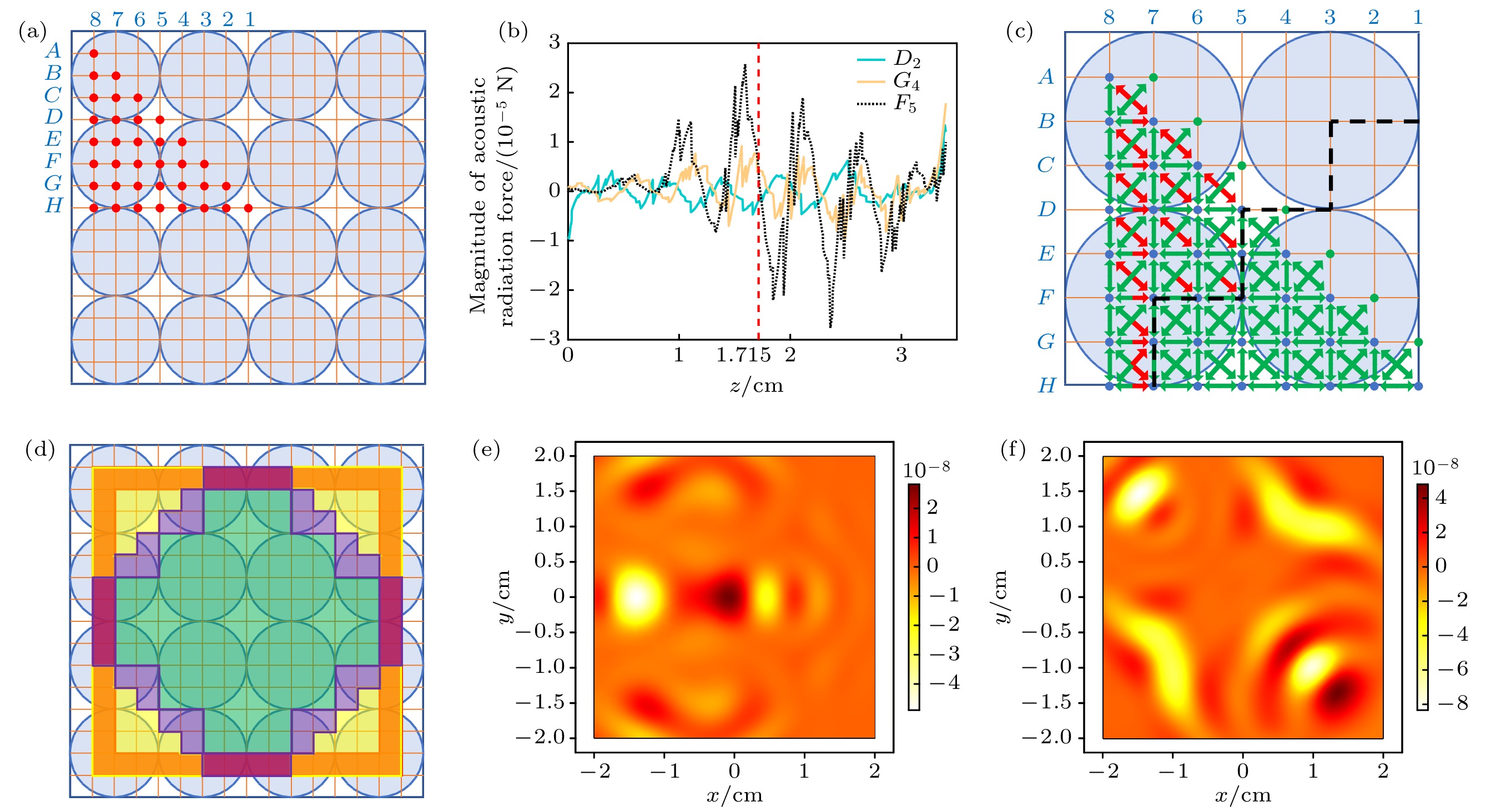图 6 (a)细化后的格点平面图, 图中的红点区域为囊括所有移动情形的最小研究区域, 格点的命名法则与之前的粗格点相同. (b)聚焦点位于细格点平面F₅处(粗格点平面C₃处)时, 格点F₅ (C₃), G₄以及粗格点平面中D₂处垂直截线上垂向声辐射力随高度的分布情况. 红色虚线标出1.715 cm高度. (c)红色箭头代表不稳定移动的路径, 绿色箭头代表稳定移动的路径. 黑色虚线右下方为稳定移动的区域, 左上方为不稳定移动的区域. (d)绿色区域为可稳定操控微粒的区域; 紫色区域内跨对角线向中心移动是不稳定的; 黄色区域内斜跨对角线向中心和向外移动是不稳定的; 红色区域内沿网格线向中心移动不稳定; 橙色区域为红、黄交叠区域, 深紫色区域为红、黄、紫交叠区域. (e), (f)聚焦点分别位于H₇和B₇处时, 操控平面上声辐射力势能的分布
Figure6. (a) Refined grid plane. The red dot area in the figure is the smallest research area that includes all moving situations. The nomenclature of the points is the same as the previous coarse grid points. (b) Distribution of vertical ARF along 3 vertical cutlines located at F₅ (C₃ in the coarse grid), G₄ and D₂ (the coarse grid) respectively. Red dashed line marks the height of 1.715 cm. The red arrows in panel (c) represent the path of unstable movement, and the green arrows represent the path of stable movement. Below the black dotted line is the stable moving area, and the rest part is the unstable moving area. The green area in panel (d) is the area where the particles can be stably manipulated. The purple, yellow and red area are areas where movement along diagonal of grids towards the center, movement along diagonal of grids towards and away from the center, movement along grid line towards the center are ubstable; orange area is the superposition of red area and yellow area, dark purple area is the superposition of red, yellow and purple area. (e), (f) Distribution of ARF potential energy on manipulation plane when the focus points are located at H₇ and B₇.

对于稳定的点, 选取中间高度$ 1.715\mathrm{?}\mathrm{c}\mathrm{m} $和力的极大值的平均高度$ 1.565\mathrm{?}\mathrm{c}\mathrm{m} $这两个具有代表性的高度来检验是否满足第2个条件. 通过逐点绘制两个高度上的力场, 发现所有满足第1个条件的点在对应的高度上均可获得向心力, 满足第2个条件, 所以这些稳定移动的路径理论上均可以实现.
将稳定与不稳定的路径绘制在图6(c)中, 可以明显地看出, 不稳定的路径集中于虚线左上部分, 虚线右下部分均可以实现定向移动. 不稳定的路径最多的是跨格点对角线的路径, 从中心向外辐射的或者从外向内汇聚的都有. 沿着格线的移动路径也有一部分属于不稳定的范畴, 它们基本是从最外围一层格线向内层移动的路径. 在聚焦点从中心H₁向顶点A₈移动的过程中, 力的汇聚区在到达D₅点之后开始明显变形, 由圆形逐渐变为椭圆形, 短轴沿着H₁—A₈方向(图6(f)). 在这样的形变下, 沿对角的路径往往是不稳定的. 而在聚焦点从经线1到经线8的垂直移动的过程中, 力的汇聚区在到达H₇点之后开始发生明显变形, 从圆形变成“包子形” (图6(e)), “包子”向中心一侧凸起, 所以微粒从最外层经线向内层经线的移动总是不稳定的. 这样来看, 不稳定的移动路径大多发生在边界处.
根据对称性, 从图6(c)延伸可得到整个操控平面上的路径稳定性情况. 图6(d)对路径进行了分类. 其中绿色覆盖的区域为完全稳定的路径, 其余部分为不稳定的移动路径. 外围有一圈红色所覆盖的区域, 代表粒子沿格线从外侧向内侧移动的路径是不稳定的; 紫色覆盖区域表示沿对角线向中心移动的路径缺乏稳定性; 黄色所覆盖的区域代表沿对角线向中心汇聚和向外发散的路径均缺乏稳定性; 交叠区域同时包含两种类型的不稳定路径. 有交叠的区域集中于最外一层的网格上, 代表了在这个区域内有多种不稳定路径的存在. 这种现象的产生在路径规划中涉及到绿色区域之外的区域时应注意回避这些路径.

本文首先建立了声压与声辐射力势能之间的直接关系, 在理论上证明了变相位声镊实现的可行性. 其次指出了变相位声镊的本质就是通过相位调制实现声压聚焦点的移动, 同时考虑了移动过程中重力的影响, 指出平面移动只是限制在一定范围内的移动. 以平面阵列声镊为例, 分析了不同移动路径下的粒子稳定性问题. 在声镊声场的不同位置, 粒子向各方向移动稳定性是不同的. 一般来说, 斜向移动和边界处的粒子移动稳定性差, 需要在实际路径规划过程中予以注意. 可以通过减小移动步长, 提高移动稳定性. 在本文算例中, 步长减小1/2, 稳定性提高近40%.
除了格点间距过大和靠近边缘处力的汇聚区发生形变会导致移动不稳定外, 平面阵列的规模也会对移动稳定性造成一定的影响. 加大阵列的规模, 使行和列都有所增加, 可以使边缘离中心更远, 从而扩大稳定移动区域的范围. 本文的工作对于变相位型声镊的研究与设计具有一定的参考意义.