1.College of Instrumentation & Electrical Engineering, Jilin University, Changchun 130026, China 2.Key Laboratory of Geophysical Exploration Equipment, Ministry of Education, Jilin University, Changchun 130026, China
Fund Project:Project supported by the Excellent Young Scientists Fund of the National Natural Science Foundation of China (Grant No. 41722405), the National Natural Science Foundation of China (Grant Nos. 41874209, 41974208), the Key Research Projects of Jilin Provincial Science and Technology Department, China (Grant No. 20180201017GX), the Science and Technology Development Projects of Jilin Province, China (Grant No. 20180520183JH), and the Interdisciplinary Program for Doctoral Students of Jilin University, China (Grant No. 101832020DJX066)
Received Date:02 December 2020
Accepted Date:07 April 2021
Available Online:07 June 2021
Published Online:20 August 2021
Abstract:Magnetic resonance sounding (MRS) has the advantage of detecting groundwater content directly without drilling, but the signal-to-noise ratio (SNR) is extremely low which limits the application of the method. Most of the current researches focus on eliminating spikes and powerline harmonic noise in the MRS signal, whereas the influence of random noise cannot be ignored even though it is difficult to suppress due to the irregularity. The common method to eliminate MRS random noise is stacking which requires extensive measurement repetition at the cost of detection efficiency, and it is insufficient when employed in a high-level noise surrounding. To solve this problem, we propose a modified short-time Fourier transform(MSTFT) method, in which used is the short-time Fourier transform on the analytical signal instead of the real-valued signal to obtain the high-precision time-frequency distribution of MRS signal, followed by extracting the time-frequency domain peak amplitude and peak phase to reconstruct the signal and suppress the random noise. The performance of the proposed method is tested on synthetic envelope signals and field data. The using of the MSTFT method to handle a single recording can suppress the random noise and extract MRS signals when SNR is more than –17.21 dB. Compared with the stacking method, the MSTFT achieves an 27.88dB increase of SNR and more accurate parameter estimation. The findings of this study lay a good foundation for obtaining exact groundwater distribution by utilizing magnetic resonance sounding. Keywords:MRS/ random noise/ modified short-time Fourier transform/ data processing
$\begin{split} {E_{{\rm{noise}}}}\left( k \right) =\;& {N_{\left( {0,1} \right)}}\left( k \right) \cdot x\left( k \right) \\ &\times \sqrt {{{\left( {\frac{{{V_{{\rm{bac}}}}\left( k \right)}}{{x\left( k \right)}}} \right)}^2} + V_{{\rm{uni}}}^2\left( k \right)} ,\end{split}$
其中, k为离散时间样本, ${N_{\left( {0, 1} \right)}}\left( k \right)$表示均值为0标准差为1 nV的高斯噪声, ${V_{{\rm{bac}}}}\left( m \right)$表示背景噪声, 考虑到结构噪声等非特定噪声的存在, ${V_{{\rm{uni}}}}\left( m \right)$为加入的均匀噪声. 图4给出了不同噪声条件下MSTFT方法对随机噪声的消除效果. 信号1中背景噪声${V_{{\rm{bac}}}}\left( m \right)$是均值为0标准差为50 nV的高斯噪声, 均匀噪声${V_{{\rm{uni}}}}\left( m \right)$是1%的理想信号值, 加入噪声后信噪比为0.68 dB. 然后应用MSTFT算法处理噪声, 图4(a)为含噪信号的高精度时频幅度谱, 噪声在时频域内随机分布, 但是对信号峰值影响较弱, 峰值出现在0 Hz附近, 幅度在300 nV以内. 沿频率轴提取各个时刻幅度和相位的最大值后重构信号, 信号时域和频域的处理结果分别如图4(b)和图4(c)所示, 其中灰色曲线表示含噪信号, 黑色曲线为采用MSTFT方法处理数据后重构的MRS信号, 红色曲线为仿真信号, 可以看出, 随机噪声成分被消除, 信号得以保留. 消噪之后提取的信号参数和SNR, RMSE如表1首行所列, 参数提取结果E0 = (200.19 ± 5.01) nV, $T_2^* $ = (149.2 ± 2.8)ms, $\Delta f$ = (–0.03 ± 0.01) Hz, 信号SNR提升为32.67 dB, RMSE为(1.03 ± 0.55) nV. 为了测试该方法在较高噪声水平下的有效性, ${V_{{\rm{bac}}}}\left( m \right)$的标准差增大为100 nV, ${V_{{\rm{uni}}}}\left( m \right)$增大为理想信号的3%, 使信号2的信噪比为–5.20 dB. 表1的中间行为MSTFT方法对信号2的消噪结果, 提取参数E0, $T_2^* $ 和$\Delta f$分别为(202.61 ± 7.90) nV, (152.0 ± 11.8) ms和(0.04 ± 0.03) Hz, SNR提高到24.01 dB, RMSE为(3.79 ± 1.89) nV. 最后, 加入干扰程度严重的随机噪声, ${V_{{\rm{bac}}}}\left( m \right)$标准差为200 nV, ${V_{{\rm{uni}}}}\left( m \right)$为5%理想信号, 信噪比降低至–11.22 dB. 从图4(h)的时间序列上看, 在随机噪声干扰较大的情况下, MSTFT方法仍然具有良好的消噪性能, 由图4(g)可以看出, 虽然随机噪声水平增大了, 但是由于其随机分布而不能在时频域产生聚集性, 因此对信号峰值处幅度和相位影响较小, 可以直接提取而不损耗信号信息. 消噪后MRS信号的参数提取结果E0为(204.12 ± 14.07) nV, $T_2^* $ 为(154.4 ± 14.5) ms, $\Delta f$为(0.04 ± 0.06) Hz, 信噪比SNR和均方根误差RMSE分别为20.81 dB和(5.81 ± 2.42) nV. 图 4 3组仿真随机噪声消噪结果图 (a)低噪声强度下仿真数据高精度时频域振幅; (b) 低噪声强度下消噪结果时域图; (c) 低噪声强度下消噪结果频域图; (d) 中噪声强度下仿真数据高精度时频域振幅; (e) 中噪声强度下消噪结果时域图; (f) 中噪声强度下消噪结果频域图; (g) 高噪声强度下仿真数据高精度时频域振幅; (h) 高噪声强度下消噪结果时域图; (i) 高噪声强度下消噪结果频域图 Figure4. The de-noising results of 3 sets of random noise simulation: (a) High-precision time-frequency domain amplitude of simulated data under low noise intensity; (b) time domain results under low noise intensity; (c) frequency domain results under low noise intensity; (d) high-precision time-frequency domain amplitude of simulated data under moderate noise intensity; (e) time domain results under moderate noise intensity; (f) frequency domain results under moderate noise intensity; (g) high-precision time-frequency domain amplitude of simulated data under high noise intensity; (h) time domain results under high noise intensity; (i) frequency domain results under high noise intensity.
E0/nV
$T_2^* $ /ms
$\Delta f$ / Hz
SNR/dB
RMSE/nV
信号1 (SNR = 0.68 dB)
200.19 ± 3.01
149.2 ± 2.8
–0.03 ± 0.01
32.67
1.03 ± 0.55
信号2 (SNR = –5.20 dB)
202.61 ± 4.90
152.0 ± 6.7
0.04 ± 0.03
24.01
3.79 ± 1.89
信号3 (SNR = –11.22 dB)
204.12 ± 5.96
154.4 ± 12.8
0.04 ± 0.06
20.81
5.81 ± 2.42
表13组仿真随机噪声消噪后参数估计情况表 Table1.The parameter estimation after de-noising of 3 sets of simulated random noise.
24.2.实测噪声与仿真信号的消噪示例 -->
4.2.实测噪声与仿真信号的消噪示例
为了进一步验证MSTFT方法的有效性, 本节进行了另一组仿真实验, 由(2)式给出的仿真信号中E0 = 200 nV, $T_2^* $ = 100 ms, $\Delta f$ = 0 Hz, ${\varphi _0}$ = 57°, 信号持续时间为256 ms, 信号长度为596. 加入在两个不同地点进行MRS实验采集的两组实测噪声数据, 由于噪声记录中既包含尖峰噪声和工频谐波噪声, 又包含随机噪声, 因此先采用统计叠加法和自适应陷波法消除尖峰噪声和工频谐波噪声[16], 只保留随机噪声, 并对随机噪声进行重采样, 使其与仿真信号长度相等. 然后采用MSTFT方法分别对两个测点数据中的一次噪声记录进行随机噪声压制, 并将结果与叠加法处理同一脉冲矩数据的结果进行对比. 由于测点2的噪声水平略高于测点1, 因此叠加法处理随机噪声时, 对测点1的每组脉冲矩数据叠加16次, 测点2的每组脉冲矩数据叠加32次. 图5给出了传统叠加法和改进短时傅里叶变换方法压制随机噪声的对比结果, 从第一列图中可以看出, 叠加法处理数据后的结果中仍残留随机噪声成分, 而图5中间列中, MSTFT方法处理单次噪声记录, 随机噪声抑制效果明显, 信号衰减趋势与仿真信号接近, 并且与传统叠加法相比, 该方法在较低信噪比下仍能提取所需信号. 图 5 叠加法和MSTFT方法消除随机噪声效果对比图 (a) 叠加法消除随机噪声时域图; (b) MSTFT方法消除随机噪声时域图; (c) 叠加法和MSTFT方法消除随机噪声频域对比图 Figure5. Comparison of the de-noising results by using stacking and MSTFT methods: (a) Results of random noise elimination by stacking in time domain; (b) results of random noise elimination by MSTFT in time domain; (c) comparison of the de-noising results by using stacking and MSTFT methods in frequency domain.
表2叠加法和MSTFT消除随机噪声提取参数结果对比 Table2.Comparison of the parameter estimation after random noise elimination by stacking and MSTFT methods.
5.实测结果本节分别采用MSTFT方法和叠加法对同一组实测MRS数据进行处理, 对比两种方法下该组实测数据的消噪结果、参数估计和MRS反演情况. 所有数据均使用吉林大学自主开发的JLMRS-I系统在吉林省长春市郊区进行采集, 该地的地磁场强度为54720 nT, 拉莫尔频率为2330 Hz. 接收线圈为边长100 m的正方形, 16个发射脉冲矩分布在240—8350 A·ms范围内, 每组脉冲矩数据采集16次. 图6所示为不同脉冲矩下原始数据及经叠加法和MSTFT方法处理后的数据随时间的变化情况. 从图6(a)中可以看出, 原始数据受噪声干扰严重, 无法辨别信号的存在. 因此采用预处理方法预先消除尖峰噪声和工频谐波噪声, 只保留随机噪声, 并对含噪数据进行重采样. 然后采用传统叠加法消除随机噪声, 结果如图6(b)所示, 可以看出不同脉冲矩下信号幅度的变化情况和衰减趋势, 但未被完全消除的随机噪声仍会对信号产生影响. 采用MSTFT方法消除单次记录的预处理数据中的随机噪声, 结果如图6(c)所示, 随机噪声抑制效果更加明显, 信号更为突出. 图 6 实测数据处理结果图 (a) 野外探测原始数据; (b) 叠加法消除随机噪声后数据; (c) MSTFT方法消除随机噪声后数据 Figure6. De-noising results of field data: (a) Original field data; (b) random noise elimination by stacking; (c) random noise elimination by MSTFT.
图7为16个发射脉冲矩中任意4个脉冲矩信号的消噪结果. 其中黑色曲线为叠加法消噪后的MRS包络信号, 红色曲线为MSTFT方法处理单次数据记录后得到的MRS包络曲线. 图7(a)和图7(c)中可以观察到指数衰减趋势, 但是图7(e)和图7(g)中SNR仍然很低. 由时域和频域消噪结果可以看出, 与叠加法相比, 经MSTFT方法压制后信号中随机噪声水平更低. 并且如图7(f)和图7(h)的内置图所示, 当信噪比越低时, MSTFT方法的优势越明显. 另外, 虽然实际测量环境中的随机噪声不是纯白噪声数据, 但MSTFT方法仍然可行. 图 7 叠加法和MSTFT方法处理4个脉冲矩信号结果对比图 (a) 时域对比结果; (b) 频域对比结果 Figure7. Comparison of the de-noising results of 4 pulse moments by using stacking and MSTFT methods: (a) Time domain comparison; (b) frequency domain comparison.
16个脉冲矩信号的参数估计情况如图8所示. 可以看出, 采用传统叠加法和MSTFT方法处理数据后提取的信号初始振幅差距很小, 但是MSTFT方法消噪后提取的信号弛豫时间比叠加法消噪后提取的弛豫时间更为准确, 两种方法消噪后信号的频率偏移在零附近波动并且变化较为平滑, 因此可以认为采用MSTFT方法抑制随机噪声后MRS信号的提取结果更为准确. 图 8 叠加法和MSTFT处理实测数据提取参数结果对比 (a) 初始振幅; (b) 弛豫时间; (c) 频率偏移 Figure8. Parameter estimation after random noise elimination of field data by using stacking and MSTFT methods: (a) Initial amplitude; (b) relaxation time; (c) frequency offset.
对两种方法消噪后提取的MRS信号分别进行初始振幅反演, 反演结果和实验地点附近的钻孔结果对比如图9所示. 可以看出, 两组数据的反演结果得到的含水层信息均与钻孔结果显示的地层结构一致. 该地点存在两个含水层, 其中主含水层位于地下12.5—24 m的细-中-粗砂孔隙介质中, 最大含水量在11%—12%之间, 次含水层位于地下38—40 m的中砂孔隙介质中, 平均含水量约为4%. 但是相比于叠加法, 由MSTFT方法消噪后的数据进行反演, 反演结果得到的含水层信息与实际更为接近, 且实验数据采集中只需进行一次探测, 提高了野外工作效率. 图 9 叠加法和MSTFT处理实测数据提取MRS信号反演结果与钻孔结果对比 (a) 叠加法; (b) MSTFT方法 Figure9. Comparison of the inversion of the field data processd by stacking and MSTFT methods respectively with the borehole log: (a) Stacking result; (b) MSTFT result.


 图 1 叠加法分别叠加1, 4, 8和16次时消除随机噪声效果时域和频域图


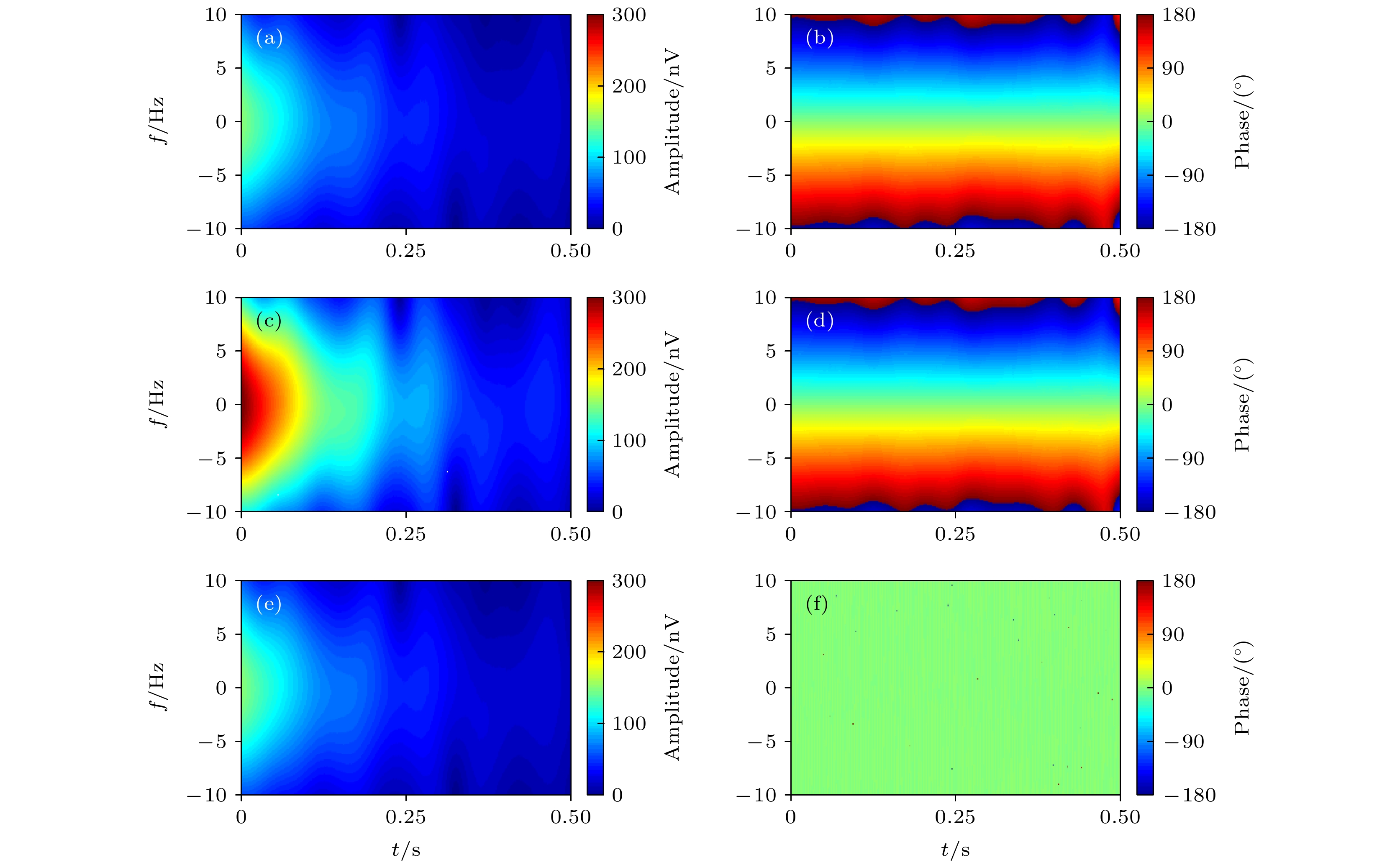 图 2 MSTFT与常规短时傅里叶变换之间的区别 (a) 时频幅度谱


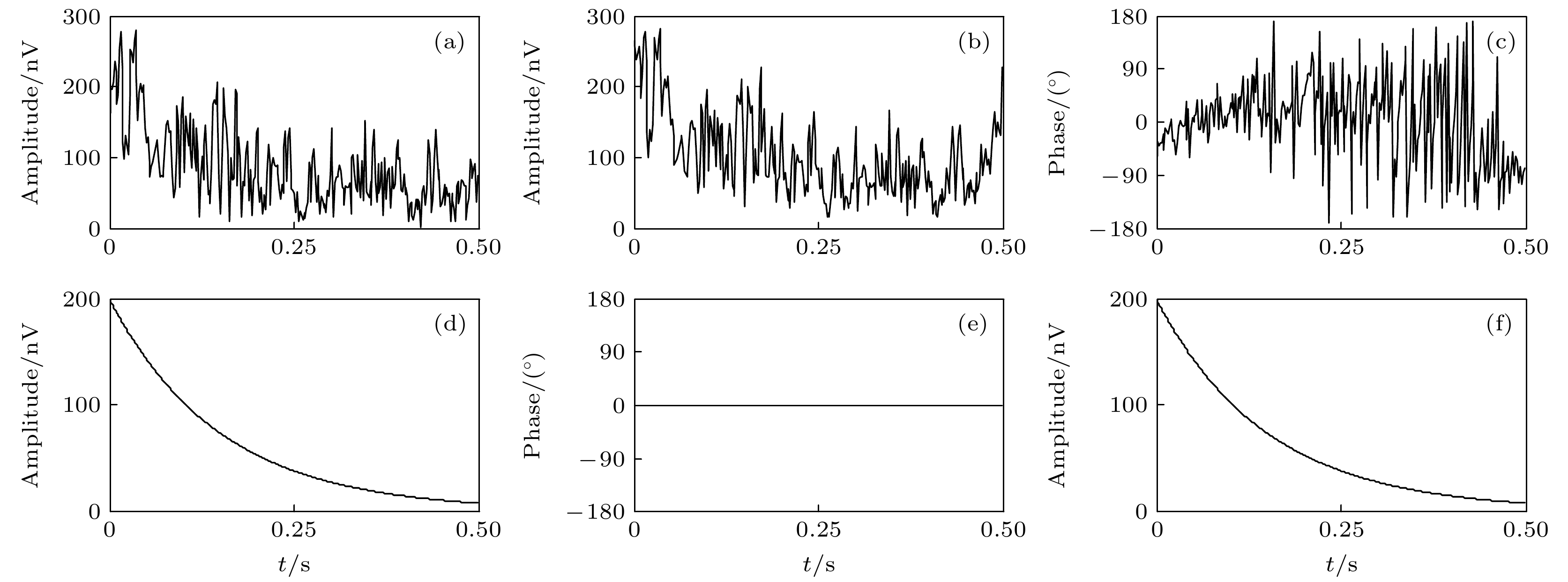 图 3 MSTFT方法消除随机噪声过程示例 (a) 仿真含噪数据; (b)瞬时幅度; (c) 瞬时相位; (d) 峰值幅度; (e) 峰值相位; (f)重构信号


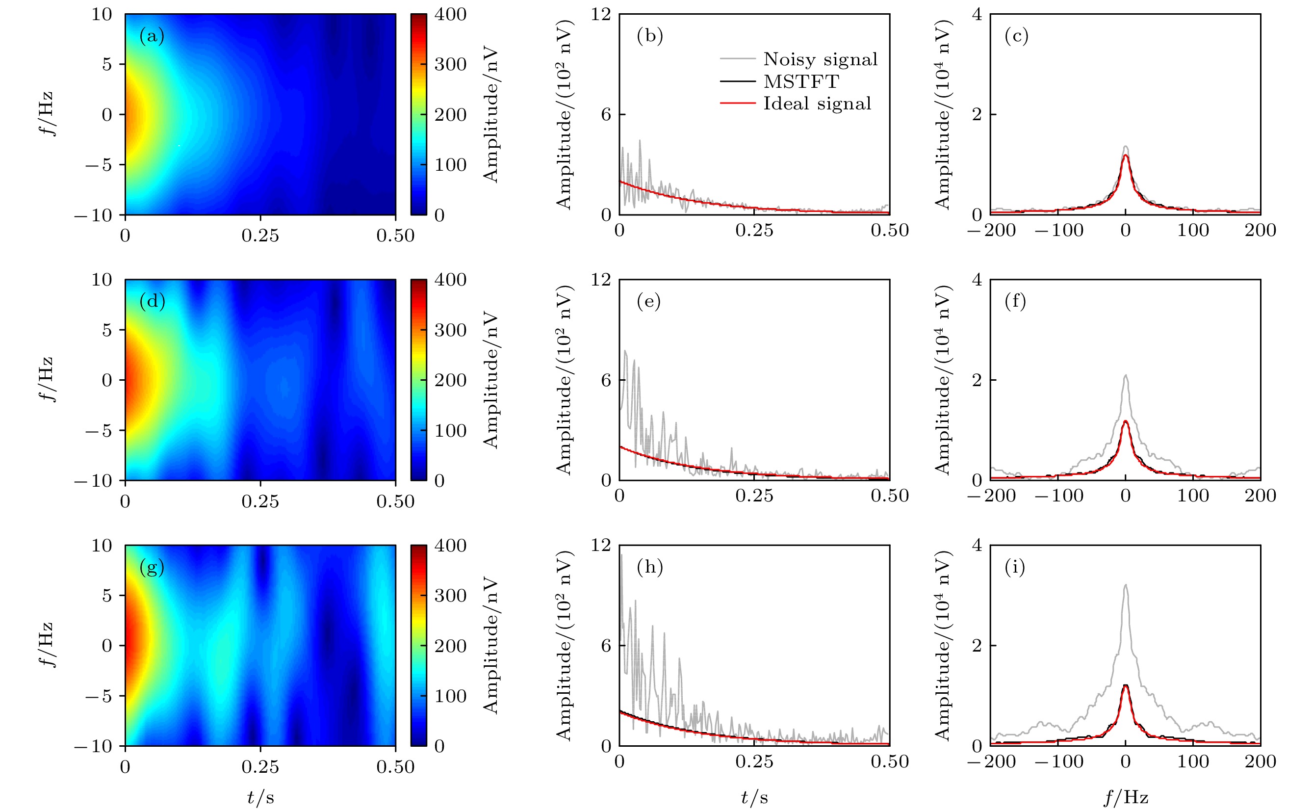 图 4 3组仿真随机噪声消噪结果图 (a)低噪声强度下仿真数据高精度时频域振幅; (b) 低噪声强度下消噪结果时域图; (c) 低噪声强度下消噪结果频域图; (d) 中噪声强度下仿真数据高精度时频域振幅; (e) 中噪声强度下消噪结果时域图; (f) 中噪声强度下消噪结果频域图; (g) 高噪声强度下仿真数据高精度时频域振幅; (h) 高噪声强度下消噪结果时域图; (i) 高噪声强度下消噪结果频域图


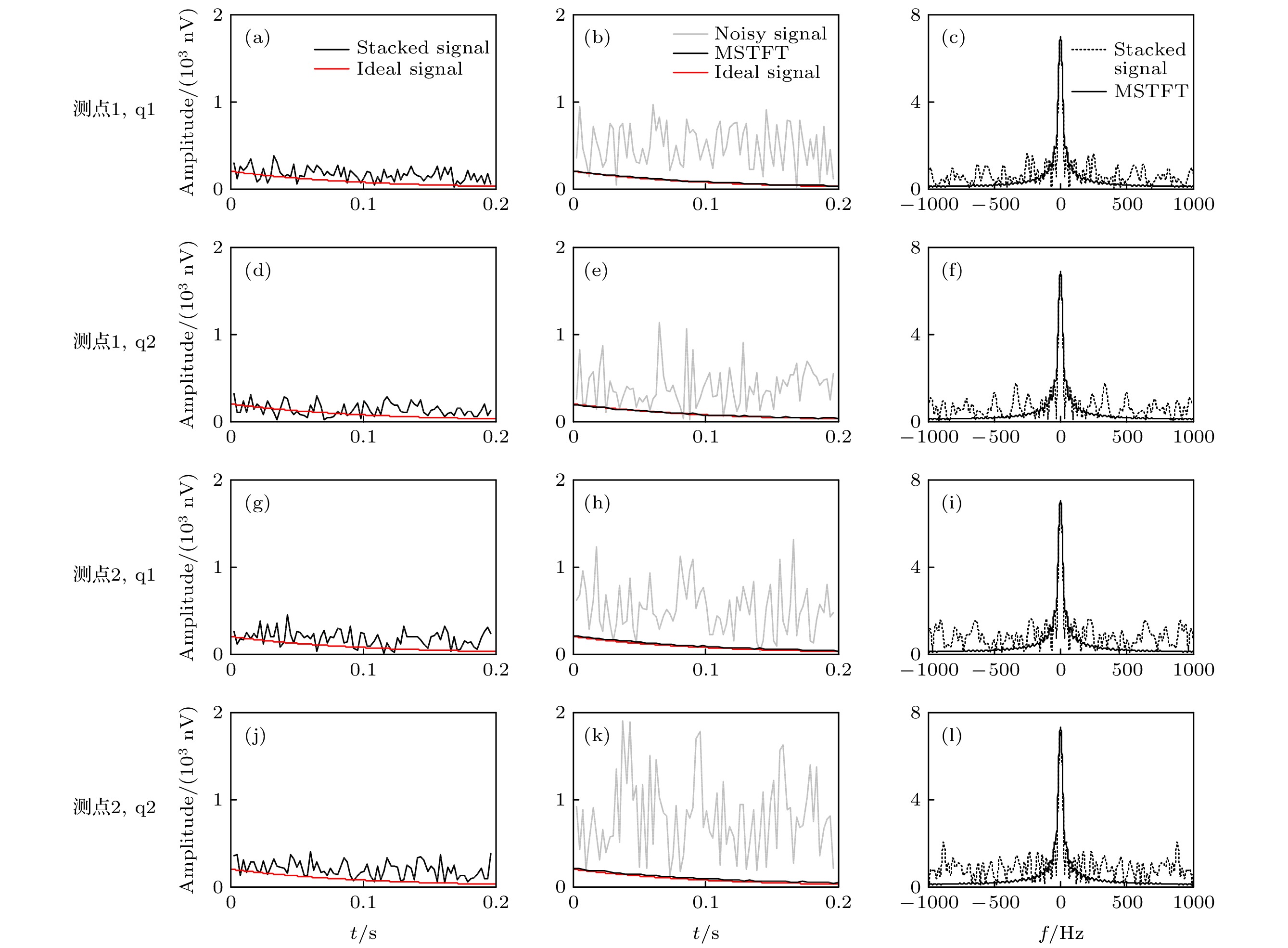 图 5 叠加法和MSTFT方法消除随机噪声效果对比图 (a) 叠加法消除随机噪声时域图; (b) MSTFT方法消除随机噪声时域图; (c) 叠加法和MSTFT方法消除随机噪声频域对比图
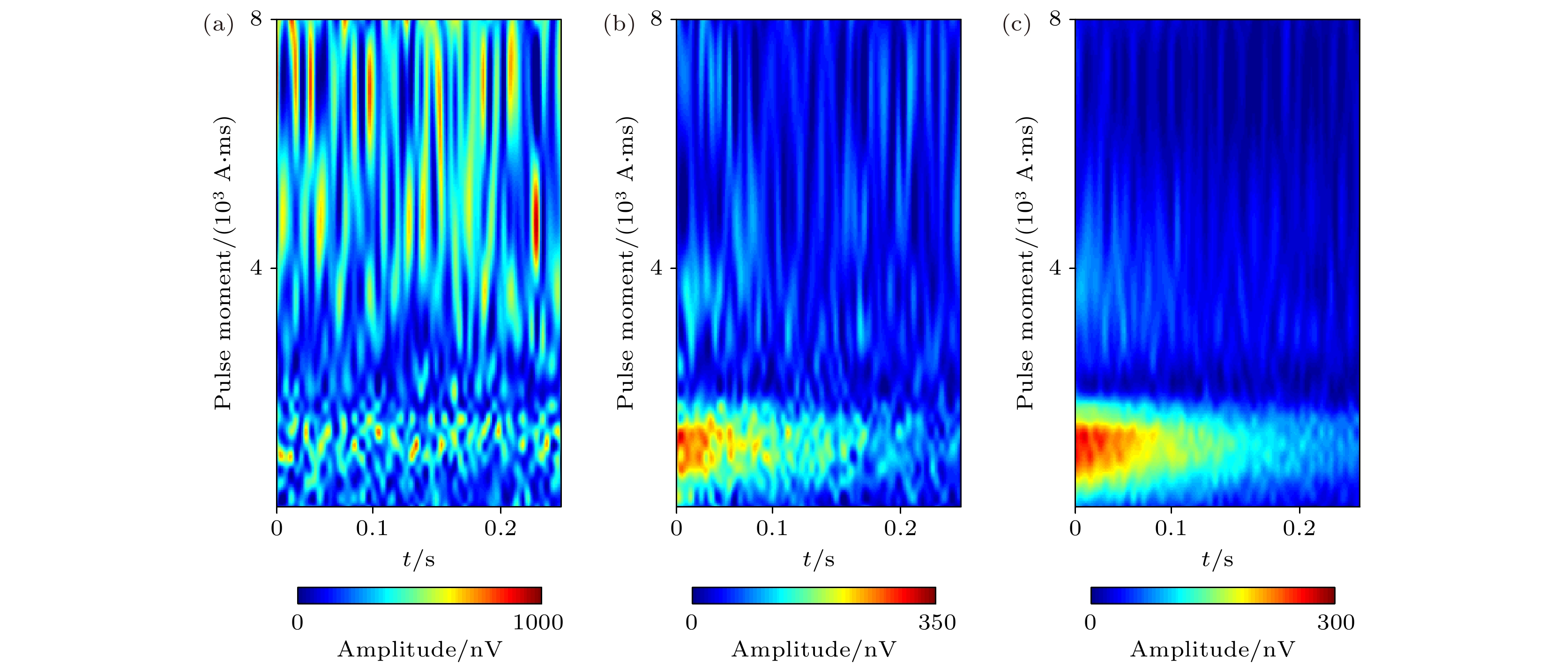 图 6 实测数据处理结果图 (a) 野外探测原始数据; (b) 叠加法消除随机噪声后数据; (c) MSTFT方法消除随机噪声后数据
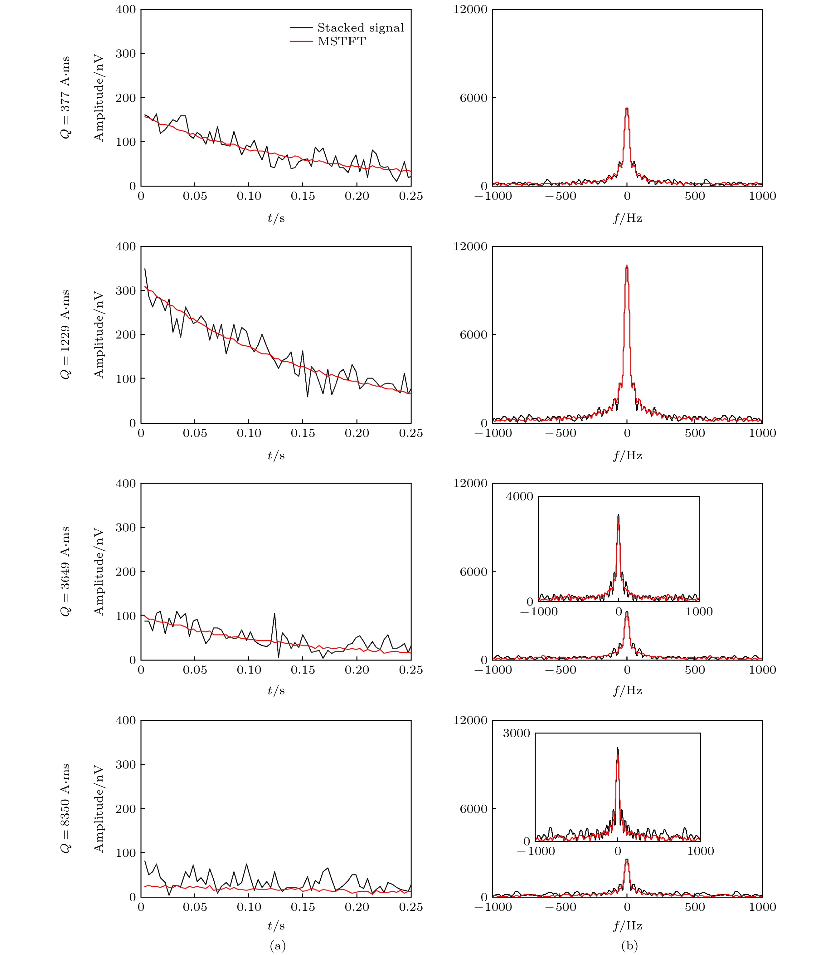 图 7 叠加法和MSTFT方法处理4个脉冲矩信号结果对比图 (a) 时域对比结果; (b) 频域对比结果
 图 8 叠加法和MSTFT处理实测数据提取参数结果对比 (a) 初始振幅; (b) 弛豫时间; (c) 频率偏移
 图 9 叠加法和MSTFT处理实测数据提取MRS信号反演结果与钻孔结果对比 (a) 叠加法; (b) MSTFT方法
