摘要:对于远程声传播问题, 地球曲率的影响不可忽略. 为分析地球曲率对远距离声传播的影响, 本文提出了一种地球曲率影响下环境参数的修正方法, 该修正方法无需改动现有声场计算模型, 具有可移植性好、计算简便的特点. 典型环境下的仿真结果表明, 由于地球曲率的影响, 在会聚区传播中, 会聚区的位置向声源方向偏移, 会聚区移动随着距离变换近似为线性关系, 1000 km距离上偏移可达10 km; 而深海声道传播中, 到达结构在时间轴上整体前移, 并伴随着在深度和时间轴上的扩展, 影响均随着传播距离的增加而逐步增大, 1000 km距离上整体前移的幅度可达136 ms.
关键词: 地球曲率/
声传播/
会聚区/
到达结构

English Abstract

全文HTML

--> --> -->

当前我国水声学研究在深远海逐渐开展, 认清深海大洋环境下的远程声传播规律对远程水声通信、远程水声导航等具有重要的意义.
在深远海环境下, 会聚区传播和深海声道传播具有相对稳定的结构, 能够高强度、远距离地传播声信号. 会聚区位置预报和深海声道传播到达结构预报是研究中重点关注的问题. Vadov^[1]发现第一会聚区的计算距离要比实验观测距离通常多出1—2 km, 他将造成这种差别的原因部分归结为传输条件的日变化. 张鹏等^[2]利用在中国南海海域收集到的一次深海声传播实验数据, 研究了深海不完全声道环境下的海底地形对海底反射会聚区位置的影响. 吴丽丽^[3]利用西太平洋海域长达1029 km的远程声传播数据, 对深海完全声道下的会聚区传播损失进行了分析, 并分析了海底深层声学结构对影区到达结构的影响. Van等^[4,5]发现脉冲声到达结构在深度上会发生扩展, 内波引起的散射很好地解释了这一现象. 张燕等^[6]利用一次南海深海声传播实验数据, 分析了深海声道轴脉冲声传播特性, 并利用简正波理论解释了不同距离和不同深度上脉冲到达结构的产生原因. 可以看到, 地形起伏、海底地质类型、传播路径上的水文变化会对会聚区传播、深海声道传播产生显著影响.
当声传播距离达到数百甚至上千公里的时候, 除了上述因素外, 地球曲率的影响同样不可忽略. 在电磁学和地震学领域, 针对地球曲率对波传播的影响问题做了充分研究. Richter^[7]将共性映射方法运用到电磁波远距离传播的地球曲率修正上. Pekeris^[8]对电磁学中地球曲率修正方法的适用性进行了分析. Muller^[9]给出了地球任意深度点源激发的体波的地球曲率近似方法, 并做出了改进^[10]. Biswas^[11,12]分析了地球曲率对瑞利波、乐甫波的影响. 在声学领域, 徐传秀等^[13]通过坐标变化, 建立了一种抛物方程模型, 并简要分析了地球曲率对声传播的影响, 结果表明地球曲率造成会聚区位置向远距离移动. Yan^[14,15]建立了考虑地球曲率影响的二维和三维的射线声学模型, 比较了地球曲率修正前后, 本征声线的到达时间和到达角度, 并发现, 地球曲率修正后, 射线路径向近距离移动. Etter^[16]给出了地球曲率的一阶修正公式, 但是并没有给出这一公式的推导过程和基于此修正方法的地球曲率对声传播的影响分析. 可以看到, 国内外在地球曲率对远程声传播的影响认识上尚有矛盾的地方, 还缺乏一种简便易用的地球曲率修正方法, 对于地球曲率对声传播的传播损失以及对到达结构的影响, 分析得也还不够到位.
本文借鉴Richer^[7]采用的共形映射方法, 推导出一种计算简便的地球曲率影响下环境参数的修正方法, 通过仿真研究了地球曲率对会聚区传播的传播损失以及深海声道传播的到达结构的影响, 并对影响规律进行了总结. 另外比较了不同地球近似模型下的修正效果. 此项研究作为远距离声传播的基础理论工作, 对认清深海大洋环境下的远程声传播规律, 开展各类应用工作都有重要的意义.

由于地球近似为一个球体, 对于远程的声传播问题, 在距离-深度平面上的声速等值面不是平行平面, 而是同心球面. 当前的声场计算都是在笛卡尔坐标系之下进行的, 在传播距离较近的情况下, 可以认为地球曲率的影响不存在. 而当距离变远的时候, 由于地球曲率造成的海洋波导的弯曲对声传播的影响将不可避免, 此时再用笛卡尔坐标系下建立的各类声场计算模型进行声场计算势必会造成输入参数与计算模型之间的失配问题.
下面对参数与模型的失配问题进行举例说明. 如图1所示, 已知声源的位置和声源的深度$ z $, 计算与声源之间距离为$ r $, 深度为$ z $的接收点A处的声压. 为了更好地说明问题, 在图1中对海洋波导的厚度进行了放大处理. 现有的方法是将参数代入到图2所示的声场计算模型进行计算. 而实际的声传播的情况如图1所示, 与声源位于同深度的接收点A不在声传播的水平直达声路径上, 我们通过声场计算模型计算的结果其实接近于接收点B的声压.
图 1 真实地球环境下的声传播形式
Figure1. The form of sound propagation in the real earth environment.

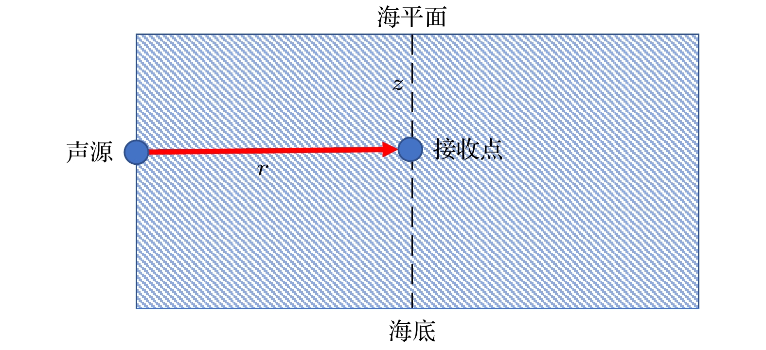图 2 仿真环境下的声传播形式
Figure2. The form of sound propagation in the simulation environment.

针对这一失配问题, 有两种解决思路. 第一种是徐传秀等^[13]和Yan^[14,15]的解决思路, 即重新构建引入地球曲率修正的二维/三维的传播模型, 但是这种方法需要对现有的各类声场计算模型进行重新编写, 工程量大, 推广起来比较困难. 另一种思路是, 在不更改现有的常用声场计算模型的情况下, 通过调整声场计算模型的输入参数, 使之适合实际的声传播情况, 从而实现地球曲率的修正. 这类方法被称为变参数媒质法^[17].
如图3所示, 假设地球为一标准球体, 地球半径为$ R=6371.03\;\mathrm{k}\mathrm{m} $ ^[18]. A点为声场中某个接收点, 坐标为$ \left(X, Z\right) $, 距离海平面的距离为$ {z}' $, 声源与接收点A之间的圆弧对应的圆心角为$ \theta $, A点距离地球球心的距离为$ a $. 与图1类似, 图3对海洋波导的厚度进行了放大处理. 要求解的亥姆霍兹方程的形式为
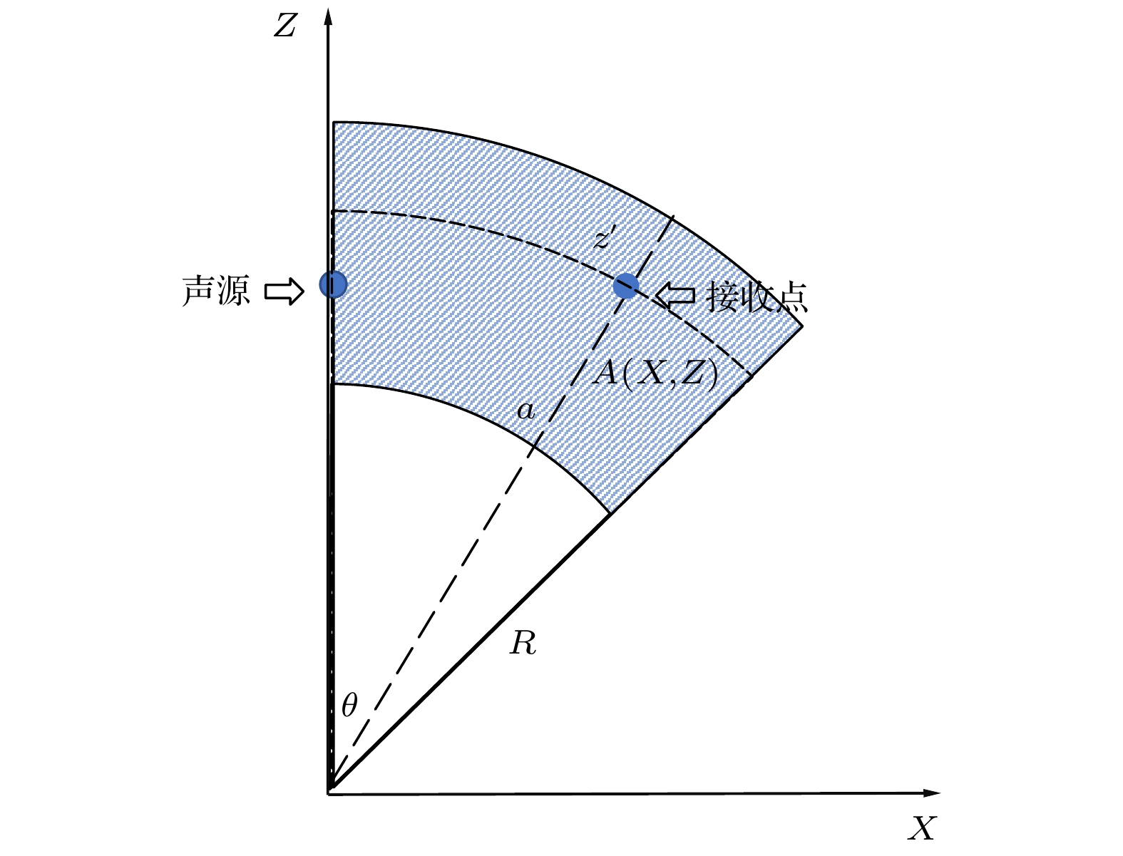图 3 极坐标系下的声传播形式
Figure3. The form of sound propagation in polar coordinate system.

$\frac{{{\partial ^2}\varphi }}{{\partial {X^2}}} + \frac{{{\partial ^2}\varphi }}{{\partial {Z^2}}} + {k^2}{n^2}\varphi = 0,$

其中$ \varphi $为位移势, $ k $为介质波数, $ n $为折射率. A点的坐标可以表示为

$\begin{split}&{X = a\;\sin \theta,}~~ {Z = a\;\cos \theta .}\end{split}$

在图4所示的笛卡尔坐标系中, A'点为图3中A点映射到笛卡尔坐标系下的点, 坐标为(x, z).
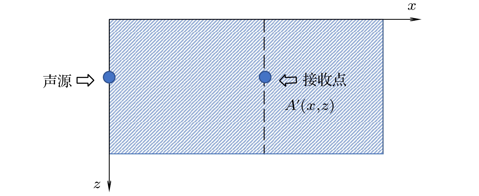图 4 笛卡尔坐标系下的声传播形式
Figure4. The form of sound propagation in Cartesian coordinate system.

设在复平面$ \zeta $和$ \xi $上, A点、A'点的坐标可以表示为

$\begin{split}&{\zeta = X + {\rm{i}}Z,}~~ {\xi = x + {\rm{i}}z.}\end{split}$

共形映射方法可以将一些不规则或者不便用数学公式表达的区域边界映射成规则的或已得到成熟分析的区域边界, 是将流体力学、弹性力学、电学等学科的实际问题化繁为简的重要方法^[19]. 将真实的地球海洋波导中的点映射到笛卡尔坐标系所采用的映射关系为^[20]

$\begin{split}&{\left( {0,{\rm{i}}R} \right) \to \left( {0,0} \right),}~~~~ {\left( {0,{\rm{i}}R{\rm{ln}}\left( {\frac{R}{a}} \right)} \right) \to \left( {0,z} \right),}\end{split}$

所以映射的形式为

$\xi = \overline {{\rm{i}}R{\rm{ln}}\left( {\frac{\zeta }{{{\rm{i}}R}}} \right)} .$

因为

$\zeta = X + {\rm{i}}Z = {\rm{i}}a{{\rm{e}}^{ - {\rm{i}}\theta }},$

得到

$\xi = R\theta + {\rm{i}}R{\rm{ln}}\left( {{R}/{a}} \right).$

因为

$a = R - z',$

等价于

$\left\{ {\begin{aligned}&{x = R\theta,}\\&{z = R \ln\left( {\frac{R}{{R - z'}}} \right).}\end{aligned}} \right.$

在共形映射中, 拉普拉斯算子的变换为^[21]

$\frac{{{\partial ^2}}}{{\partial {x^2}}} + \frac{{{\partial ^2}}}{{\partial {z^2}}} = {\left| {\frac{{{\rm{d}}\zeta }}{{{\rm{d}}\xi }}} \right|^2}\left( {\frac{{{\partial ^2}}}{{\partial {X^2}}} + \frac{{{\partial ^2}}}{{\partial {Z^2}}}} \right).$

在新的坐标系下, 二维的亥姆霍兹方程变为

$\frac{{{\partial ^2}\varphi }}{{\partial {X^2}}} + \frac{{{\partial ^2}\varphi }}{{\partial {Z^2}}} + {k^2}{n^2}{\left| {\frac{{{\rm{d}}\zeta }}{{{\rm{d}}\xi }}} \right|^2}\varphi = 0,$

其中

$\left| {\frac{{{\rm{d}}\zeta }}{{{\rm{d}}\xi }}} \right| = {{\rm{e}}^{ - \tfrac{z}{R}}} = \frac{R}{{R - z'}}.$

引入折射率修正参数$ m $,

$m = n\left( {\frac{{R - z'}}{R}} \right),$

得到了映射到笛卡尔坐标系下的亥姆霍兹方程

$\frac{{{\partial ^2}\varphi }}{{\partial {x^2}}} + \frac{{{\partial ^2}\varphi }}{{\partial {z^2}}} + {k^2}{m^2}\varphi = 0.$

根据折射率修正公式可以得到声速的修正表达式为

$c = c'\frac{R}{{R - z'}},$

其中$ c $为修正后的声速, $ {c}' $为修正前的声速.
从上面的推导可以看到, 需要调整的声场参数有3个, 分别是从声源到接收点的距离$ r $, 接收点的深度$ z $和声速$ c $.
对于距离$ r $, 在真实地球环境下的$ r $调整后, 为$ r=R\theta $, 也就是以$ \theta $为圆心角, $ R $为半径的弧长. 在没有进行地球曲率修正的时候, $ r $的计算是通过确定声源与接收点两点的经纬度坐标, 计算两点间的测地线路径的距离得到的, 修正后仍然遵循这一计算方法.
综上, 地球曲率修正公式表示为

$\begin{aligned}&{z = R{\rm{ln}}\left( {\frac{R}{{R - z'}}} \right),}\\&{c = c'\left( {\frac{R}{{R - z'}}} \right).}\end{aligned}$

将深度$ z $和声速$ c $修正后的表达式进行泰勒级数展开得到:

$\begin{aligned}&{z = z' + \frac{{{z^{\prime 2}}}}{{2R}} + \frac{{{z^{\prime 3}}}}{{3R}} + \frac{{{z^{\prime 4}}}}{{4R}} + \ldots,}\\&{c = c'\left( {1 + \frac{{z'}}{R} + \frac{{{z^{\prime 2}}}}{{{R^2}}} + \frac{{{z^{\prime 3}}}}{{{R^3}}} + \cdots } \right).}\end{aligned}$

因为地球上海洋的平均海深为3734 m, 深度超过8000 m深度的海域面积只占到全部海域面积的0.04%^[22]. 所以$ {z}'/R\ll 1 $, 对泰勒级数展开式取一阶近似可得:

$\begin{aligned}&{z = z' + \frac{{{z^{\prime 2}}}}{{2R}},}\\&{c = c'\left( {1 + \frac{{z'}}{R}} \right).}\end{aligned}$

(18)式与Etter^[16]给出的修正方法一致. 运用此方法进行地球曲率修正, 计算修正后的声场, 误差来源有两部分. 一部分是上述一阶近似引入的误差, 但因为海深远小于地球半径, 此误差可以忽略. 另外一部分就是环境参数修正后, 运用声场计算模型计算时产生的误差.
修正后的深度$ z $是在真实海深$ {z}' $的基础上, 加上一个修正项得到的. 也就是说, 修正后的深度$ z $要略大于真实深度$ {z}' $, 修正后深度相较于修正前深度的差值会随着深度的增加逐渐变大. 修正后的声速变化情况与深度类似.
采用深海中典型Munk剖面^[23]来比较修正前后的声速剖面的变化情况. Munk剖面的表达式为

$C\left( z \right) = {c_0}\left\{ {1 + \varepsilon \left[ {{{\rm{e}}^{ - \eta }} - \left( {1 - \eta } \right)} \right]} \right\},$

其中$\eta = {2\left(h-{h}_{0}\right)}/{B}$, $ {h}_{0} $为声道轴的深度, $ B $为波导的垂直宽度, $ {c}_{0} $为声速最小值(声道轴处), $ \varepsilon $描述了偏移极小值的量级. 采用Munk给出的典型数据, $B=1300\;\mathrm{m}, \;{z}_{0}=1300\;\mathrm{m},\; {c}_{0}=1500\;\mathrm{m}/\mathrm{s},\; \varepsilon = $$ 0.00737$.
由图5可以看到, 地球曲率修正后的声速剖面在同深度的声速值要大于未修正的声速剖面的声速值. 在较浅的深度, 修正前后的声速剖面差异不明显, 在深海, 修正前后的声速剖面有较大的差异. Munk剖面地球曲率修正前后在深海的声速梯度对比如图6所示, 可以看到, 修正前后深海声速梯度变化明显.
图 5 地球曲率修正前后Munk声速剖面对比
Figure5. Comparison of Munk sound speed profiles before and after the earth curvature correction.

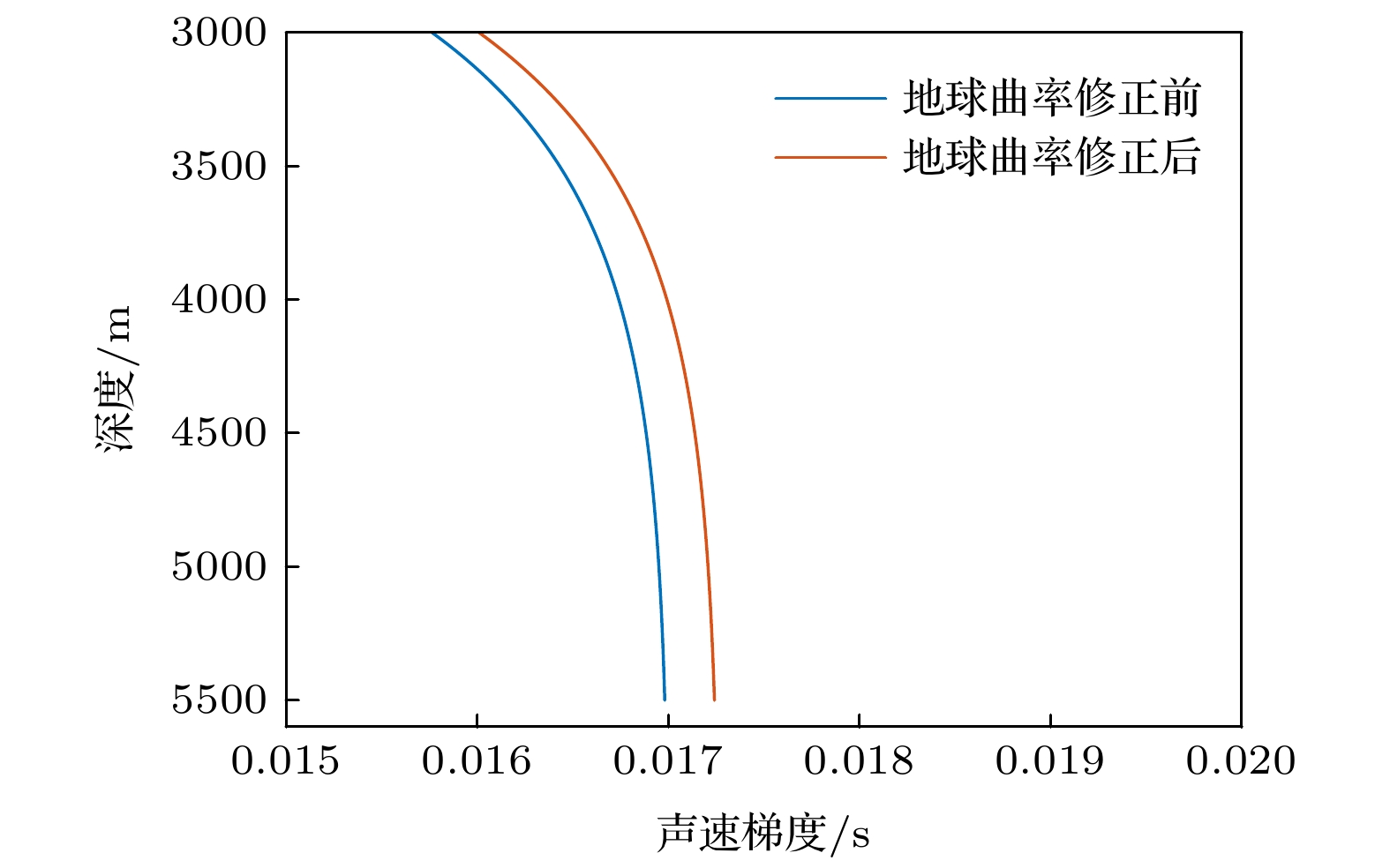图 6 地球曲率修正前后Munk声速剖面在深海声速梯度对比
Figure6. Comparison of sound velocity gradient of Munk sound velocity profile before and after earth curvature correction in deep sea.

会聚区是深海中良好的声信道, 在实际的水声探测、通信中有较广泛的应用. 以下通过仿真研究地球曲率对会聚区传播损失的影响. 仿真的声速剖面是上文提到的Munk声速剖面, 采用的海底模型包含两层液态海底, 由一层沉积层和半无限基底组成. 如图7所示, 沉积层厚度为$ 100\;\mathrm{m} $, 声速为$ 1550\;\mathrm{m}/\mathrm{s} $, 密度为$ 1.65\;\mathrm{g}/{\mathrm{c}\mathrm{m}}^{3} $, 吸收系数为$ 0.1\;\mathrm{d}\mathrm{B}/\lambda $. 基底中声速为$ 1800\;\mathrm{m}/\mathrm{s} $, 密度$ 1.9\;\mathrm{g}/{\mathrm{c}\mathrm{m}}^{3} $, 吸收系数为$ 0.1\;\mathrm{d}\mathrm{B}/\lambda $.
图 7 仿真采用的海底模型
Figure7. Seabed model used in simulation.

图8给出了抛物方程近似声场模型(RAM-PE)^[24]计算的引入地球曲率修正前后不同深度上的声传播损失(transmission loss, TL)随距离的变化情况对比. 仿真设置声源深度为$ 200\;\mathrm{m} $, 中心频率$ 100\;\mathrm{H}\mathrm{z} $, 计算的频带带宽为$ 23\;\mathrm{H}\mathrm{z} $, 频点数为11. 仿真的最远距离为$ 1000\;\mathrm{k}\mathrm{m} $. 从图8可以看到, 修正前后都出现了明显的会聚区传播现象.
图 8 二维传播损失图　(a)地球曲率修正前; (b)地球曲率修正后
Figure8. Numerical TL: (a) Before the earth curvature correction; (b) after the earth curvature correction.

不同深度下的地球曲率修正前后的传播损失对比如图9所示, 图9(a)对应的是会聚区传播的情况. 可以看到, 相较于未修正前, 会聚区位置前移, 并且随着距离的增大, 前移的距离越来越大. 图9(b)和图9(c)代表中层深度的情况, 地球曲率修正前后的传播损失曲线没有明显的变化规律. 图9(d)展示了5000 m深度上的会聚区传播中下反转点区域的地球曲率修正前后的传播损失变化情况, 可以看到, 进行地球曲率修正后, 传播损失曲线变化情况与200 m深度时类似.
图 9 不同接收深度下的地球曲率修正前后的传播损失对比　(a) 200 m; (b) 1000 m; (c) 2000 m; (d) 5000 m
Figure9. Comparison of TL before and after correction of earth curvature at the three different receiver depths: (a) 200 m; (b) 1000 m; (c) 2000 m; (d) 5000 m.

图10给出了地球曲率修正前后不同深度和不同距离传播损失的差值, 可以看到清晰的类似会聚区分布的图样, 体现出地球曲率导致会聚区整体向前移动的趋势, 不同的深度上, 影响程度不同. 在500—3500 m左右的深度, 修正前后传播损失相差不大. 会聚区传播的下反转点深度位置处, 地球曲率修正前后, 传播损失差异较大.
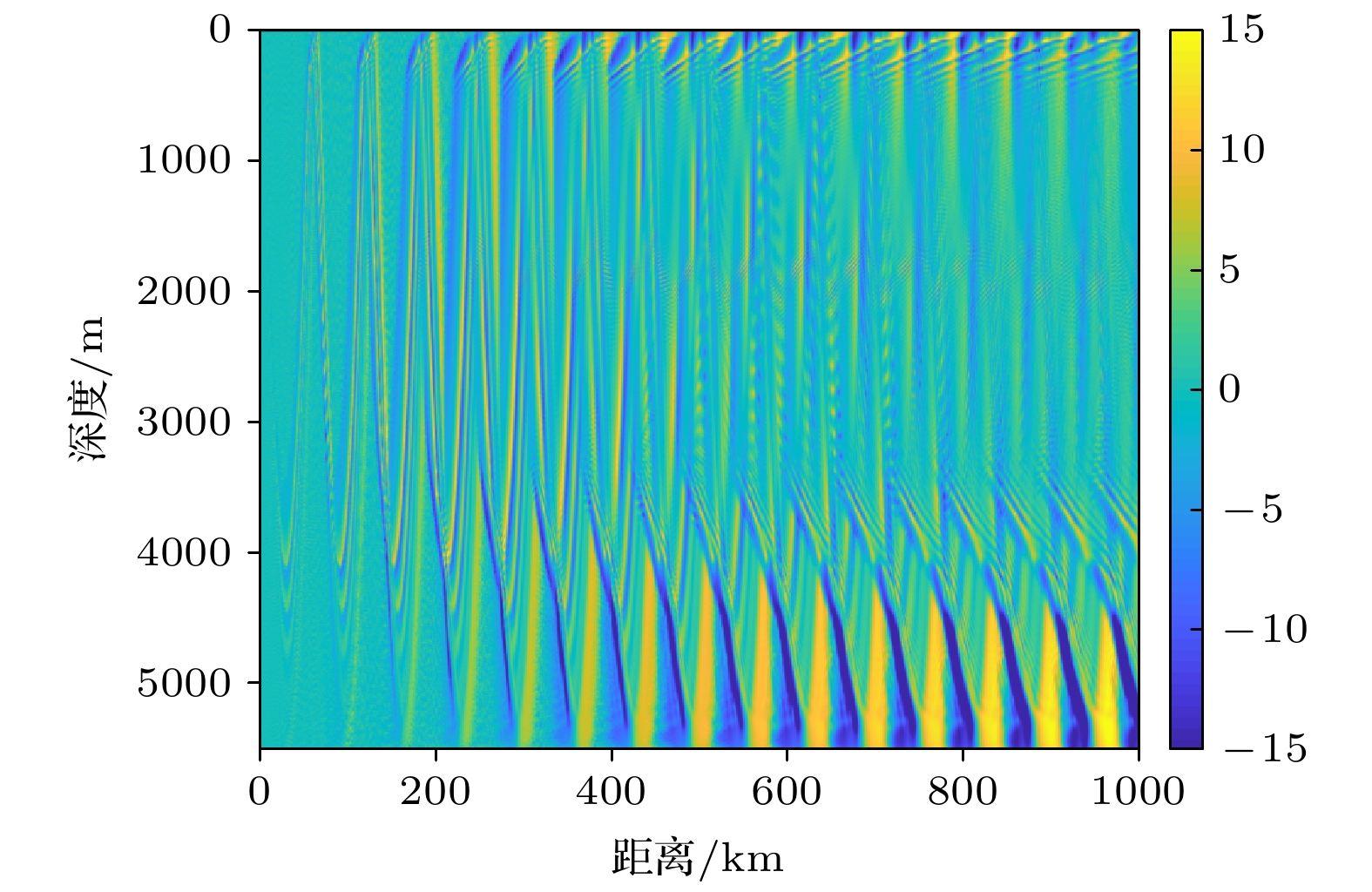图 10 地球曲率修正前后传播损失的差值
Figure10. The difference of the TL before and after the earth curvature correction.

王彦磊等^[25]对西北太平洋的声速剖面进行了分类, 选取文中提到的四种典型的西太平洋声速剖面, 分别命名为Ⅰ型声速剖面(130°E, 15°N), Ⅱ型声速剖面(150°E, 10°N), Ⅲ型声速剖面(135°E, 25°N)和Ⅳ型声速剖面(155°E, 35°N), 位置分布如图11所示. 声速剖面根据WOA(world ocean atlas)^[26,27]数据库得到.
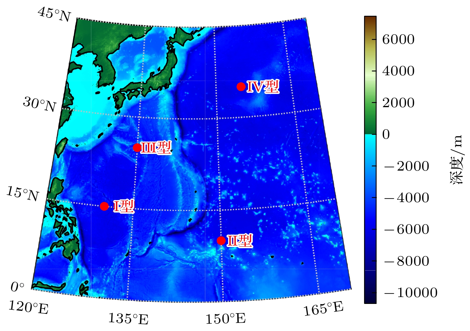图 11 西北太平洋四类典型声速剖面的分布位置
Figure11. Distribution locations of four typical sound speed profiles in the Northwest Pacific.

图12给出的是西北太平洋四类典型的声速剖面图, 可以看到, 四类声速声道均为深海完全声道, 具备实现会聚区传播的条件.
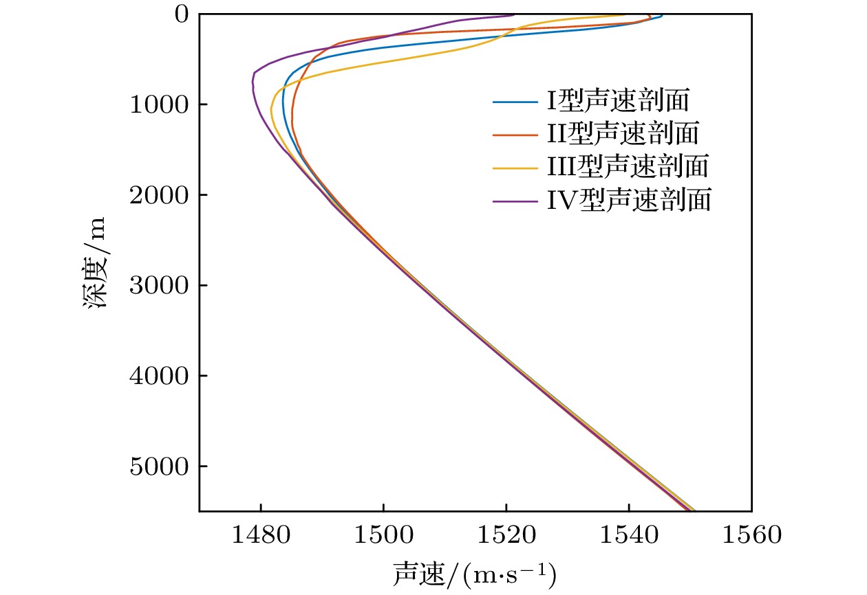图 12 西北太平洋四类典型声速剖面
Figure12. Four types of typical sound speed profiles in the Northwest Pacific.

仿真设置声源深度为200 m, 中心频率100 Hz, 频带带宽23 Hz, 计算的频点数为11. 仿真的最远距离为1000 km. 海底模型如图6所示. 图13给出的是200 m深度的接收情况. 可以看到, 四类不同的声速剖面环境下, 均出现了明显的会聚区传播现象. 地球曲率修正后, 会聚区向声源方向前移, 前移的幅度随着距离的增大而逐渐增大. 这一结论与Munk剖面下的仿真结果相同.
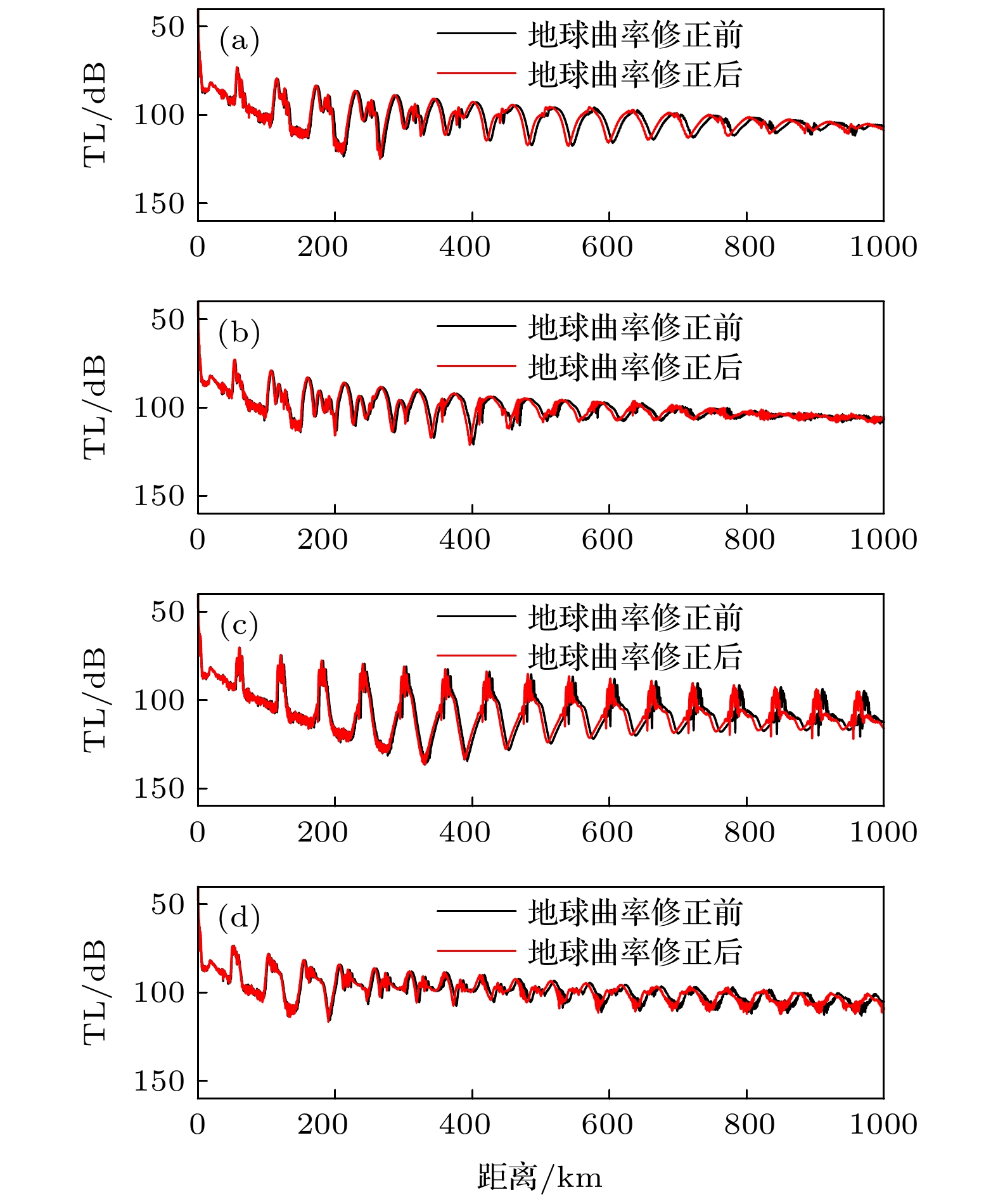图 13 西北太平洋四类典型声速剖面的200 m深度的传播损失　(a)Ⅰ型声速剖面的传播损失; (b) Ⅱ型声速剖面的传播损失; (c) Ⅲ型声速剖面的传播损失; (d) Ⅳ型声速剖面的传播损失
Figure13. TLs at a depth of 200 m in four types of typical sound speed profiles in the Northwest Pacific: (a) TLs of type Ⅰ sound speed profile; (b) TLs of type Ⅱ sound speed profile; (c) TLs of type Ⅲ sound speed profile; (d) TLs of type Ⅳ sound speed profile.

定义地球曲率修正前的各个会聚区传播损失峰值所在的位置为会聚区的位置. 针对某个特定会聚区, 先大致划分该会聚区所在的区间, 然后对该区间内的地球曲率修正前的传播损失曲线和地球曲率修正后的传播损失曲线做互相关处理, 根据互相关曲线的极大值出现的位置相较于中心点的偏移, 得到一个偏移量, 将这个偏移量定义为该会聚区在进行地球曲率修正后的会聚区偏移量. 经过上述方法处理, 得到了各类声速剖面下的各个会聚区的偏移值, 如图14所示.
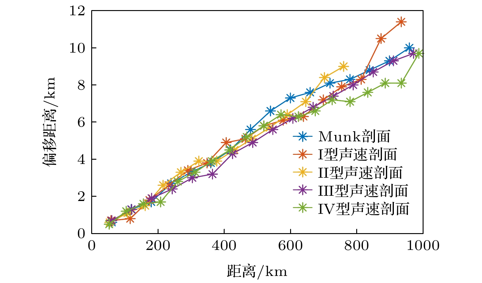图 14 不同的声速剖面下计算的会聚区移动情况
Figure14. Movement of the convergence zone calculated under different sound speed profiles.

由图14可以看到, 不同声速剖面下, 相同距离上, 地球曲率修正后的会聚区偏移程度相近, 传播200 km距离会聚区偏移2 km左右, 传播500 km距离会聚区偏移5 km左右, 传播1000 km的距离会聚区偏移可达10 km. 对某特定的声速剖面, 会聚区偏移随距离变化呈现近似的线性关系, 随距离变大, 地球曲率会导致会聚区偏移程度越来越大, 传播距离每增长100 km, 会聚区偏移增加约1 km.

深海声道, 又被称为SOFAR声道, 在大洋层析、远程水声导航等领域中有重要应用. 仿真设置的海洋环境为前文所述的Munk剖面, 声源深度为1300 m, 仿真时采用的声源脉冲$ S\left(t\right) $^[28]为

$S\left( t \right) = \left\{ {\begin{aligned}&{\frac{1}{2}\sin \left( {{w_{\rm{c}}}t} \right)\left[ {1 - \cos \frac{1}{4}({w_{\rm{c}}}t}) \right],\;0 < t < \frac{4}{{{f_{\rm{c}}}}}}\\&{0,\;\;\;\;\;\;\;\;\;\;\;\;\;\;\;\;\;\;\;\;\;\qquad\qquad\qquad{\text{其他},}}\end{aligned}} \right.,$

这是Hanning加权的四周期正弦波. 声源的中心频率$ {f}_{\mathrm{c}} $为200 Hz, 脉冲的时间窗长度为10 s. 以下通过仿真分析了不同距离上的脉冲到达结构.
图15给出了归一化后1000 km距离处地球曲率修正前后的到达结构, 图中不同颜色体现了到达脉冲的相对强弱. 可以看到, 地球曲率对到达结构产生的主要影响有三点. 1)地球曲率使得到达结构在时间轴上整体前移, 前移的幅度约为136 ms. 这是因为地球曲率修正后, 声速剖面的声速略大于修正前的声速导致的. 2)受地球曲率影响, 地球曲率修正后得到的到达结构相较于修正前, 出现了整体的扩展, 包括深度方向上的延拓和时间方向上的展宽, 越靠近到达结构左侧, 展宽程度越大. 这是也是因为修正后声速增大, 导致部分声线路径的传播时间变短, 有些路径的声线会比之前先到达接收点. 3)地球曲率使得各个深度上的多途结构的能量分布也发生了变化.
图 15 1000 km距离上的到达结构　(a)地球曲率修正前; (b)地球曲率修正后
Figure15. Arrival structure at 1000 km: (a) Before the earth curvature is corrected; (b) after the earth curvature is corrected.

图16比较了500, 1300和2500 m三个深度上归一化处理后的地球曲率修正前后的接收时域波形. 如图16(b)所示, 地球曲率修正前后, 接收的时域波形明显前移, 前移幅度约为140 ms. 并且由于地球曲率修正后到达结构整体的展宽以及能量的变化, 导致部分深度到达的时域波形产生明显的差异, 如图16(a)和图16(c)所示.
图 16 地球曲率修正前后1000 km距离上的不同接收深度的时域到达波形比较　(a) 500 m; (b) 1300 m; (c) 2500 m
Figure16. Comparison of time-domain arrival waveforms at 1000 km before and after the earth curvature correction at different receiver depths: (a) 500 m; (b) 1300 m; (c) 2500 m.

图17和图18比较500和2000 km距离上的地球曲率修正前后的到达结构. 从不同距离的到达结构的比较可以看到, 1000 km距离上地球曲率对到达结构产生的三类主要影响在各个距离上都有体现, 并且影响程度都随着传播距离的增大逐渐增大.
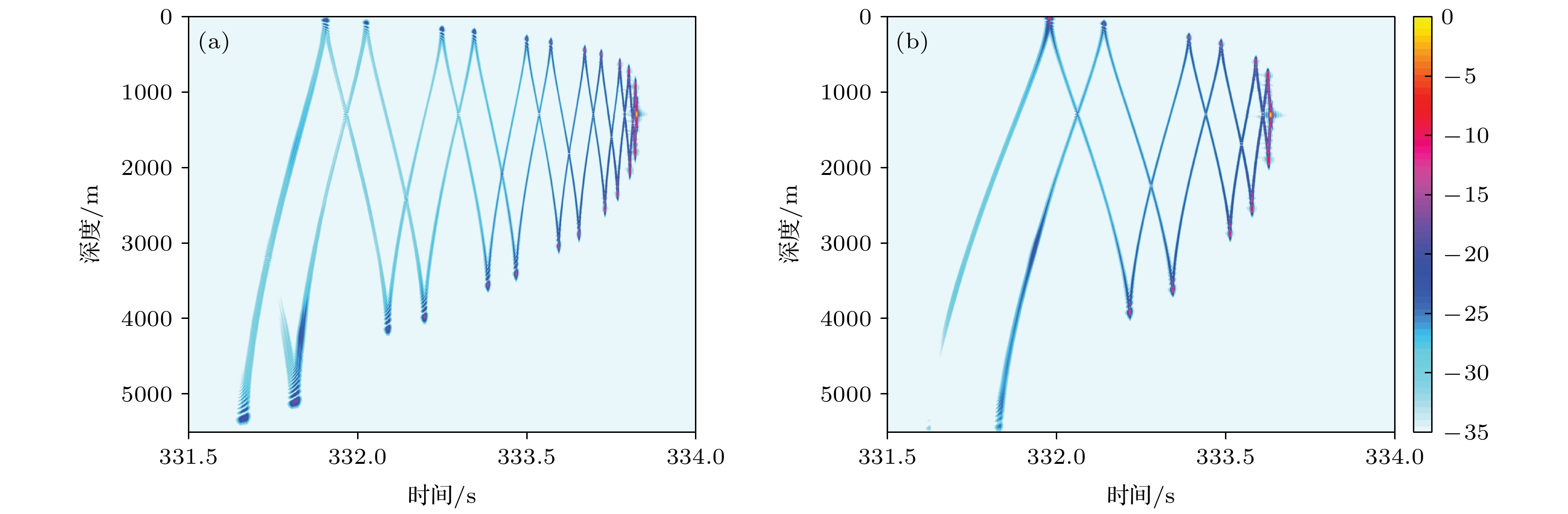图 17 500 km距离上的到达结构　(a)地球曲率修正前; (b)地球曲率修正后
Figure17. Arrival structure at 500 km: (a) Before the earth curvature is corrected; (b) after the earth curvature is corrected.

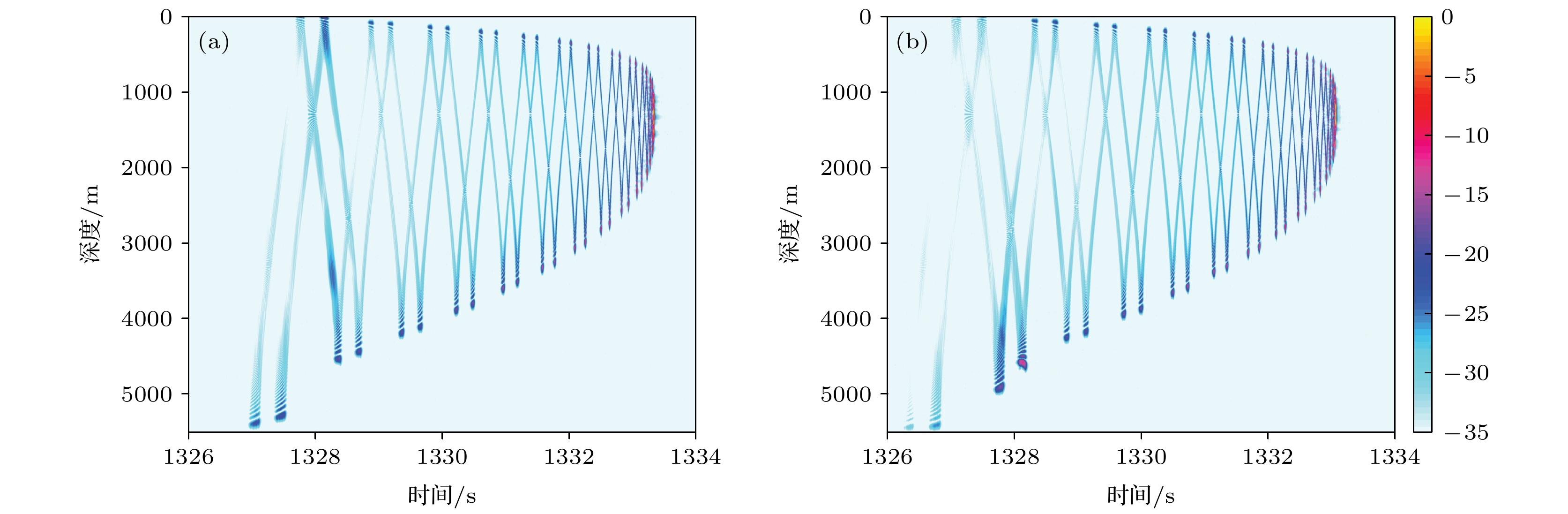图 18 2000 km距离上的到达结构　(a)地球曲率修正前; (b)地球曲率修正后
Figure18. Arrival structure at 2000 km: (a) Before the earth curvature is corrected; (b) after the earth curvature is corrected.

以上的分析都是在将地球近似为标准球体时进行的. 而实际上, 地球是一个扁平的椭球体, 如图19所示. 国际上对地球椭球建立了不同的数学模型^[18], 这些数学模型对应不同的地球椭球参数, 比较著名的有贝塞尔椭球、克拉克椭球、克拉索夫斯基椭球、以及全球定位系统(GPS)所使用的WGS84椭球, WGS84椭球也是最常用的地球椭球.
图 19 地球椭球模型
Figure19. Earth ellipsoid model.

WGS84椭球对应的地球椭球参数为^[18]: 子午椭圆的长半轴$a= 6378.137\;\mathrm{k}\mathrm{m}$; 子午椭圆的短半轴$b= 6356.752\;\mathrm{k}\mathrm{m}$; 子午椭圆的扁率$\alpha =({a-b})/{a} $$ =1/298.2572$; 子午椭圆的第一偏心率$e={\sqrt{{a}^{2}-{b}^{2}}}/{a}$; 子午椭圆的第一偏心率${e}'={\sqrt{{a}^{2}-{b}^{2}}}/{b}$.
在WGS84椭球下, 有几种常用的地球曲率半径, 包括子午线曲率半径、卯酉线曲率半径、平均曲率半径和任意方向上的曲率半径.
子午圈曲率半径定义为子午圈上一点的曲率半径, 设为$ M $,

$M = {{a\left( {1 - {e^2}} \right)}}/{{{W^3}}},$

其中$ W=\sqrt{1-{e}^{2}{\mathrm{sin}}^{2}B} $, $ B $为大地纬度.
卯酉圈是与子午面垂直的闭合圆圈, 卯酉圈的曲率半径用$ N $来表示:

$N = {a}/{W}.$

平均曲率半径$ {R}_{\mathrm{a}} $是指经过曲面任意一点所有可能方向上的法截线曲率半径$ {R}_{\mathrm{A}} $的算数平均值. 推导得到曲面上任意一点的平均曲率半径表示为

${R_{\rm{a}}} = \sqrt {MN} .$

图20给出了从赤道到极地的地球平均曲率半径变化情况. 赤道上地球平均曲率半径最小, $ {R}_{0} $为6356.863 km, 随着纬度的升高, 地球平均曲率半径增大, 到极点上平均曲率半径取最大值, $ {R}_{90} $为6399.699 km.
图 20 地球平均曲率半径随纬度的变化情况
Figure20. The variation of the average radius of curvature of the earth with latitude.

下面分析不同地球半径取值对地球曲率影响下环境参数修正方法的影响. 设$ {c}_{\mathrm{a}} $为地球平均半径下经过地球曲率修正后的Munk剖面的声速值, $ {c}_{0} $为赤道位置上地球平均曲率半径下经过地球曲率修正后的Munk剖面的声速值, $ {c}_{90} $为极点位置上地球平均曲率半径下经过地球曲率修正后的Munk剖面的声速值,
图21给出了由于地球半径选取造成的修正后的声速剖面的差异. 可以看到, 三种声速剖面几乎完全重合. 5000 m深度上, 三类声速剖面之间的差值在$ {10}^{-3} $ m/s量级, 在实际计算中, 此差异造成的影响可以忽略. 所以将地球近似为一标准球体进行地球曲率修正, 完全可以满足修正后计算精度的需要.
图 21 选取不同地球半径计算声速剖面的比较
Figure21. Comparison of sound speed profiles calculated by selecting different earth radius.

本文提出了一种计算简便的地球曲率影响下环境参数的修正方法, 并对地球曲率对声传播的影响进行了分析, 主要结论如下.
1)对于会聚区传播, 地球曲率会造成会聚区位置相对于未修正前的计算位置前移, 偏移程度随着距离的增大而增大, 1000 km距离上偏移可达10 km. 通过对不同的声速剖面仿真结果分析得到, 会聚区移动随距离变化近似为线性关系, 传播距离每增大100 km, 会聚区的偏移增加约1 km.
2)对于深海声道传播, 地球曲率会导致到达结构整体向前移动, 前移的幅度随着距离的增大而逐渐增大, 1000 km距离上整体前移的幅度可达136 ms. 地球曲率还会造成整个到达结构在深度和时间方向上的扩展. 在特定深度上接收到的时域波形在地球曲率修正前后有较大差异.
3)比较不同地球近似模型下的修正效果表明, 将地球近似为标准球体即可满足计算精度需要.
以上工作是以水平不变的环境为前提进行分析的, 以后将进一步研究水平变化海洋环境下的地球曲率对声传播以及远程信息传输的影响.