1.College of Instrumentation and Electrical Engineering, Jilin University, Changchun 130061, China 2.Key Laboratory of Geophysical Exploration Equipment, Ministry of Education (Jilin University), Changchun 130061, China
Fund Project:Project supported by the National Key Research and Development Project of China (Grant No. 2019YFC0409105), the National Natural Science Foundation of China (Grant No. 41874209), the Jilin Provincial Projects for Key Science and Technology, China (Grant No. 20180201017GX), the Jilin Provincial Projects for International Cooperation, China (Grant No. 20200801007GH), and the Cultivate Foundation for Outstanding Youth of Jilin University, China (Grant No. 45120031D015)
Received Date:28 August 2020
Accepted Date:20 November 2020
Available Online:02 March 2021
Published Online:20 March 2021
Abstract:Surface magnetic resonance sounding (MRS) has generally been considered to be an efficient tool for hydrological investigations. As is well known, the effective relaxation time $ T_2^*$ which characterizes the decay rate of MRS free-decay-induction (FID) signal and is used to measure pore-scale properties, is particularly limited for several special cases (e.g. areas with magnetic rock subsurfaces). Recent years, the transverse relaxation time $ T_2$ obtained from spin-echo signal was adopted to implement the surface MRS, and showed great potentials for estimating the porosity and permeability. However, owning to the short period of development, the related modeling and inversion strategies are rarely introduced and summarized. Actually, the general practice for surface MRS $ T_2$ measurement fits the spin-echo by the exponential function and the fitting line was directly used as the FID signal for inversion. This scheme not only limits the precision of interpretation, but also loses part of valid information about original field data. Aiming at these problems, in this paper, we introduce the calculation of forward model and thus a two-stage framework with singular value decomposition (SVD) linear inversion involved is derived to quantify the $ T_2$ distributed with depth. Considering the fact that the inversion result of SVD is always strongly affected by the noise level, an improved method which combines the simultaneous iterative reconstruction technology (SIRT) with SVD is proposed. To be specific, we compare the measurement schemes with kernel functions between $ T_2$ and the original theory in MRS, and then provide the forward and inversion formulations. In order to substantiate the effectiveness of this method, we conduct the synthetic experiments for Carr-Purcell-Meiboom-Gill sequence and explain the dataset with the mentioned strategies. As expected, the combined approach possesses a better performance in shallow layer with an error of 1.5% and 0.02 s for water content and $ T_2$ for the contaminated data, respectively. With these advantages, it is expected to realize the adoption of the SVD with SIRT in field applications and further investigate the aquifer characterizations in the future. Keywords:surface magnetic resonance sounding/ spin-echo/ T2 forward and inversion/ linear spatial inversion
为对比FID与SE探测区别, 验证重聚脉冲对激发过程的影响, 计算了同一配置下, 两种激发方式的横向磁化强度分布(发射、接收线圈均为边长100 m方形、单匝), 结果见图2. 由于采用同一激发脉冲(2 A·s), 二者的横向磁化强度分布趋势相似, 但在效率上, 由于SE信号接收发生在FID信号之后, 其理论幅值明显低于FID信号. 在上述结果基础上, 仿真二者的一维灵敏度核函数, 即分别将横向磁化强度(2)式、(8)式代入灵敏度核函数表达式(6)式, 并按层状大地结构积分, 如图3(a)和图3(b)所示. 由图可知, 对应于横向磁化强度分布, SE信号的灵敏度核函数幅值也相对降低. 图 2 2 A·s激发脉冲下的地面磁共振(a) FID与(b) SE激发横向磁化强度分布剖面(实验配置为100 m方形发射/接收线圈, 单匝; 填充颜色表示激发横向磁化强度相对于总磁化强度比例) Figure2. Excitation profile (2 A·s) for (a) FID and (b) SE responses in a surface MRS case with 100 m square transmitting/receiving loop, 1-turn configuration. Color indicates the amplitude ratio of the excited transverse magnetization to the total magnetization.
图 3 单匝100 m方形发射/接收线圈探测配置下的地面磁共振(a) FID与(b) SE一维灵敏度核函数(填充颜色反映在对应于激发脉冲矩, 某一固定深度下存在地下水能够诱发得到的磁共振信号幅度) Figure3. Comparison of kernel function with 100 m transmitting/receiving square loop, 1-turn configuration for (a) FID and (b) SE excitation. Color reflects the signal amplitude induced by underground water at a given depth layer corresponding to each pulse moment.
其中, z对应于一维大地层深, ${t_n}$为第n个SE信号达到峰值的时刻. 图4为典型含水结构下的FID与SE磁共振响应(地下8—20 m存在单一含水层, 含水量最大30%, 对应$T_2^*$或${T_2}$为400 ms). 由于对应SE信号(图4(b))的灵敏度核函数整体幅度偏低, 且随着接收时间增大幅度逐渐衰减, 所以对应于同一含水模型其整体幅度明显低于FID信号(图4(a)), 且伴随每一次重聚脉冲发射, 呈现多峰值分布. 值得注意的是, 图4仿真中认为含水层$T_2^*$ = ${T_2}$, 根据前文的(3)式, 实际情况下的$T_2^*$应略小于${T_2}$, 但由于此处仅用于对比FID与SE响应形式、量级上的差别, 故并没有严格区分二者间的大小. 图 4 单匝100 m方形发射/接收线圈探测配置下, 同一含水情况下的地面磁共振响应(a) FID与(b) SE信号(填充颜色反映对应激发脉冲矩, 其FID或SE信号随时间衰减的磁共振信号幅度) Figure4. Comparison of forward responses for the same aquifer distribution, with 100 m transmitting/receiving square loop, 1-turn configuration for (a) FID and (b) SE excitation. Color reflects the signal amplitude induced by underground water decays with receiving time corresponding to each pulse moment.
其中, j是当前的迭代次数. 随着迭代进行, 拟合与实测数据误差不断缩小, 最终可求得地下水SE分布矩阵m. 将前文中SVD反演结果(图5)代入SIRT进一步迭代拟合, 如图6所示. 可以看到, 对于无噪声情况下的数据反演, SIRT方法可有效弥补SVD的误差, 其反演结果几乎与原始模型一致(图6(a)). 在分别加入3 nV (图6(b))与6 nV (图6(c))高斯白噪声情况下, 单一SVD方法仅能反演得到前两个地下水自旋回波, 其边缘分辨率极低, 且非含水区域受噪声残留影响, 形成多处明显的波动. 对于反演得到的数据尾部, 已几乎难以判定第4、第5自旋回波是噪声残留还是信号. 应用SIRT方法进一步处理上述反演结果, 能够明显提升前两个自旋回波的边缘分辨率, 并识别最末的自旋回波信号, 压制非含水区域残留噪声引起的波动. 图 6 (a)模型与其在(b) 3 nV和(c) 6 nV高斯白噪声情况下的SVD与SIRT联合线性空间反演结果 Figure6. (a) Simulated modeling and its linear spatial inversion results employing SVD and SIRT with (b) 3 nV and (c) 6 nV Gaussian noise.
为验证与SVD联合处理过程中, SIRT策略的收敛特性, 基于图6数据计算过程, 同时比较了不同噪声情况下的迭代次数(图7). 受噪声波动影响, 含噪声幅度越大, 反演得到的最终数据误差也相应增大, 但收敛所需的迭代次数基本维持不变(约100次), 这说明了本文提出的策略用于地面MRS自旋回波反演时, 始终维持着快速收敛的特性. 图 7 不同噪声情况下, SIRT线性空间反演迭代次数与拟合误差间的关系 Figure7. Relationship between iteration and fitting errors for SIRT linear spatial inversion with different noise cases.
为得到最终的w与${{{T}}_2}$分布, 单独提取对应于每层的地下水SE信号包络, 并结合其峰值信息, 进行单指数或多指数拟合. 为了降低原始数据中残留噪声及求解误差对拟合的影响, 在上述拟合过程中, 通常还需考虑加入窄时间窗, 即分别以$t = 2\tau, $$ 4\tau, 6\tau, \cdots$时间点为中心, 取一定范围内包络幅值平均量作为拟合峰值, 其过程如图8所示[19]. 图 8 地面磁共振SE信号线性空间反演及含水量-横向弛豫时间分布拟合示意图 Figure8. Schematic diagram of linear spatial inversion and non-linear fitting of water content and transverse relaxation time for surface MRS spin-echo responses.
虽然SE探测主要应用在非均匀地磁场分布情况下, 其地下电阻率与拉莫尔频率分布并不均匀. 但本节的仿真实验目的为验证本文反演方法有效性, 故可忽略以上非均匀性带来的影响. 设定地磁场强度为54721 nT, 拉莫尔频率(即设定的激发频率)为2330 Hz, 地磁倾角与地磁偏角分别为60°, 0°. 探测线圈采用边长为100 m的方形线圈, 发射与接收均为单匝, 探测空间为线圈正下方(地下)电阻率为100 Ω·m的均匀半空间. 由于SE信号的探测激发效率略低于FID, 由此设定反演最大深度为60 m, 激发脉冲为[0.1 8]A·s间按指数取样的40组交流脉冲, 重聚脉冲为其倍数, 即分布在[0.2 16]A·s间, 对应每个激发脉冲发射5次重聚脉冲, 其间隔参数$\tau = 83\;{\rm{ms}}$. 结合选取的探测深度及激发脉冲矩, 设定分布在–5 m至–15 m、–30 m至–50 m的两个含水层, 背景含水量与横向弛豫时间分别设定为1%和0.02 s, 如图9(a). 根据该含水模型拟合得到的每层最大w分别为30%和50%, 对应${T_2}$为0.4 s和0.5 s. 考虑到选取的参数$\tau $及重聚脉冲个数, 设定模拟信号的采样时间为0.8 s. 由于野外MRS探测数据信噪比通常较低, 即使经过硬件及算法多重噪声压制策略, 依旧残留部分噪声. 为给实际的野外勘探提供参考经验, 同时验证本文反演方法的抗干扰特性, 向模拟数据中加入3 nV的高斯白噪声, 则根据上述含水模型计算得到的加噪MRS信号包络, 如图9(b)所示. 由于本文为仿真实验, 且其探究重点是SE信号的建模过程及反演解释, 故信号响应图中没有展示激发脉冲所引起的FID信号. 但在实际野外的SE探测实验中, 不仅能够在MRS数据初始段观测到FID信号, 且在后续SE信号解释前, 还需首先排除接收FID信号对SE包络提取的干扰. 图 9 (a)地面磁共振CPMG探测实验模型与(b)正演数据(加入3 nV高斯白噪声), 假设地下存在两个含水层, 分别分布在–5 m至–15 m及–30 m至–50 m. Figure9. (a) Simulated modeling and (b) dataset (adding 3 nV Gaussian noise) for CPMG sequence assuming a surface MRS experiment with two aquifers, which distributed from –5 m to –15 m and –30 m to –50 m, respectively.
24.2.反演结果 -->
4.2.反演结果
作为对比, 仿真数据首先由SVD方法单独处理. 前文提及的吉洪诺夫正则化及滤波器截断方案被应用于该反演过程. 为保证反演结果具有实际水文地质意义, 将病态矩阵导致的m矩阵负值元素, 均用零替代. 如图10(a)所示, 经过反演过程, SE响应由时间-脉冲间的函数关系转换为时间-深度间函数关系. 在噪声影响下, 地下水SE信号成像质量较差, 甚至在地下12 m左右出现“断层”, 尽管能够通过该反演结果大致判断两含水层存在位置, 但各个地下水SE信号边缘分辨率较低. 尤其对于深层含水层, 其各个SE的幅度远低于真实情况, 且几乎无法分辨含水区域与非含水区域的界限. 此外, 在模型中并不存在地下水区域, 均分布着明显噪点, 且在地下20 m处, 出现2 m左右的“假”含水层. 图 10 加入3 nV高斯白噪声的地面磁共振仿真数据SVD线性空间反演结果 (a) 地下水SE响应随深度及接收时间的变化; (b)与(c)分别为应用15 ms时间窗(单指数)拟合得到的w与T2分布结果 Figure10. Linear spatial inversion results of SVD method for synthetic surface MRS experiment data with 3 nV Gaussian noise polluted: (a) SE responses of underground water separated as a function of depth z and decayed over time, while the amplitude scale to water content; (b) and (c) are the subsurface w and T2 distribution fitted (mono-exponential) from (a) with a time window of 15 ms.
由于原模型并不存在多弛豫分量情况, 故仅通过单指数对图10(a)中地下水SE信号进行拟合(15 ms时间窗), 得到w及${{{T}}_2}$结果如图10(b)以及图10(c)所示. 对比原始模型拟合结果, 仅通过SVD反演能够相对精准地求得第一个含水层的含水量信息, 但由于浅层m矩阵中大量噪点的存在, 由其拟合得的${{{T}}_2}$几乎毫无规律, 第一个含水层对应的${{{T}}_2}$信息几乎被淹没. 在地下20 m处, 由于m矩阵中“假”含水层的存在, 对应含水量与${{{T}}_2}$均呈现小范围突变. 对于第二个含水层, 虽然通过其w拟合结果基本能够识别该含水层位置, 但含量远低于真实值, 对应${{{T}}_2}$信息也并不准确. 在50 m深度后, 其w与${{{T}}_2}$信息更呈现出完全相反的趋势(含水量随深度降低, ${{{T}}_2}$随深度升高), 与真实情况偏差极大. 应用本文提出的SVD与SIRT联合策略处理上述数据, 在经过98次迭代后, 反演结果基本达到稳定, 如图11(a)所示. 正如预期, 联合策略对浅层含水层几乎实现了完全还原, 在深部含水层成像上, 虽然其边缘分辨率稍有降低, 但依旧明显高于SVD方法单独反演的结果. 采用与前文相同手段提取该m矩阵的w及${{{T}}_2}$信息, 对应结果如图11(b)和图11(c)所示. 由于第一个含水层的m矩阵成像质量更高, 其w及${{{T}}_2}$信息也拟合较好, 几乎与原始模型完全重合, 它们最大误差仅为1.5%和0.02 s. 对于深层含水层, 由于m矩阵中该部分的边缘分辨率略低, 所以对应含水层的边缘部分拟合结果稍有振荡, 但w与${{{T}}_2}$信息基本还原了真实情况, 对应峰值处误差仅为5%和0.08 s. 图 11 加入3 nV高斯白噪声的地面磁共振仿真数据SVD与SIRT线性空间反演结果 (a) 地下水SE响应随深度及接收时间的变化; (b)与(c)分别为应用15 ms时间窗(单指数)拟合得到的w与T2分布结果 Figure11. Linear spatial inversion results of SVD and SIRT method for synthetic surface MRS experiment data with 3 nV Gaussian noise polluted: (a) SE responses of underground water separated as a function of depth z and decayed over time, while the amplitude scale to water content; (b) and (c) are the subsurface w and T2 distribution fitted (mono-exponential) from (a) with a time window of 15 ms.


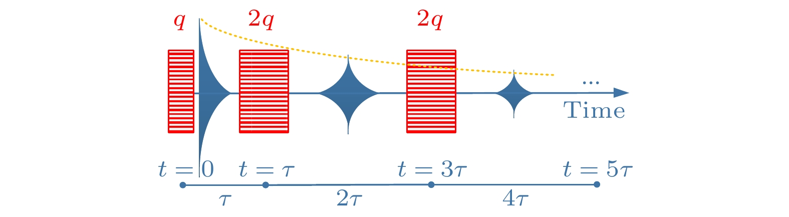 图 1 地面磁共振CPMG序列激发示意图(为获取包含T2衰减信息的完整SE信号, 发射激发脉冲q, 并间隔时间τ重复发射多个重聚脉冲2q, 重聚脉冲间的间隔为2τ)


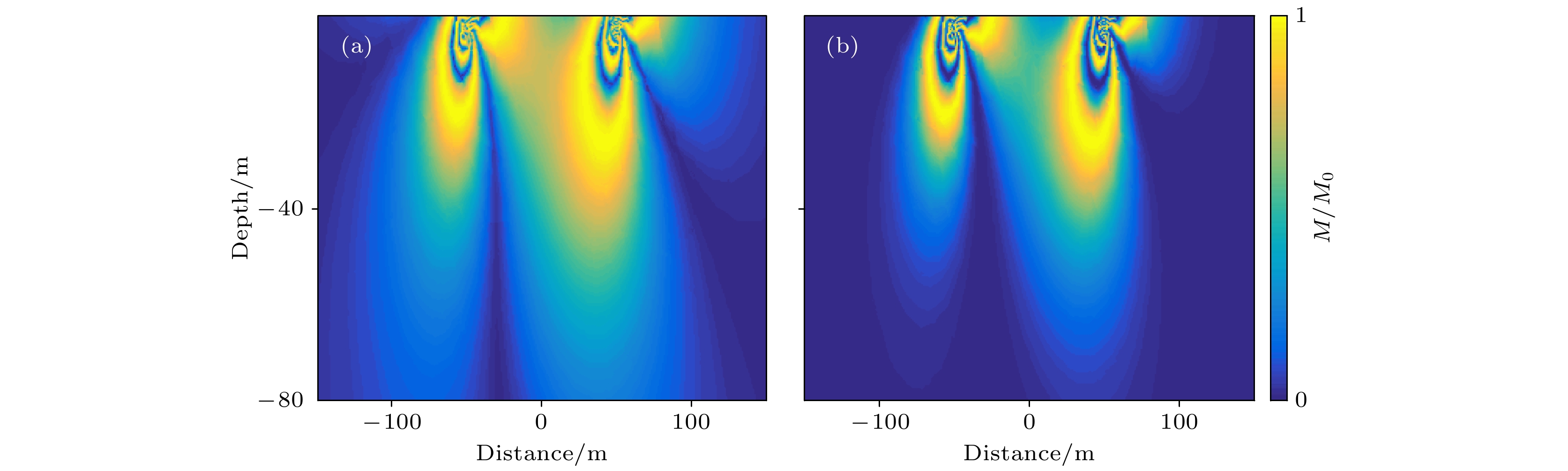 图 2 2 A·s激发脉冲下的地面磁共振(a) FID与(b) SE激发横向磁化强度分布剖面(实验配置为100 m方形发射/接收线圈, 单匝; 填充颜色表示激发横向磁化强度相对于总磁化强度比例)
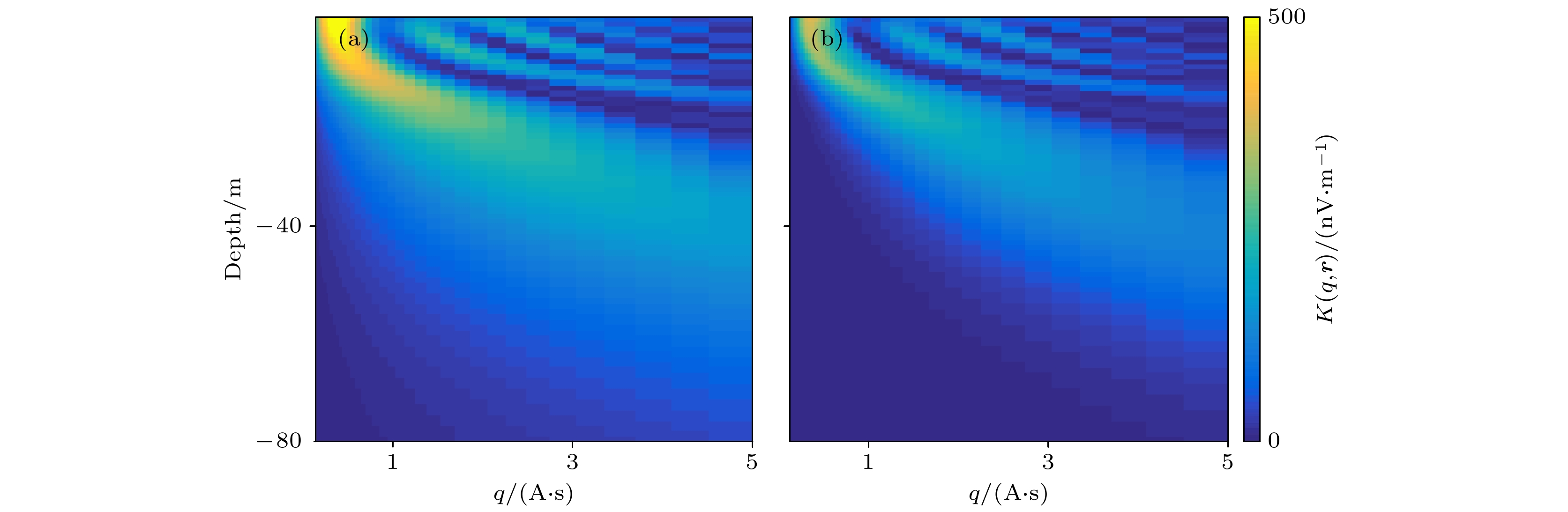 图 3 单匝100 m方形发射/接收线圈探测配置下的地面磁共振(a) FID与(b) SE一维灵敏度核函数(填充颜色反映在对应于激发脉冲矩, 某一固定深度下存在地下水能够诱发得到的磁共振信号幅度)


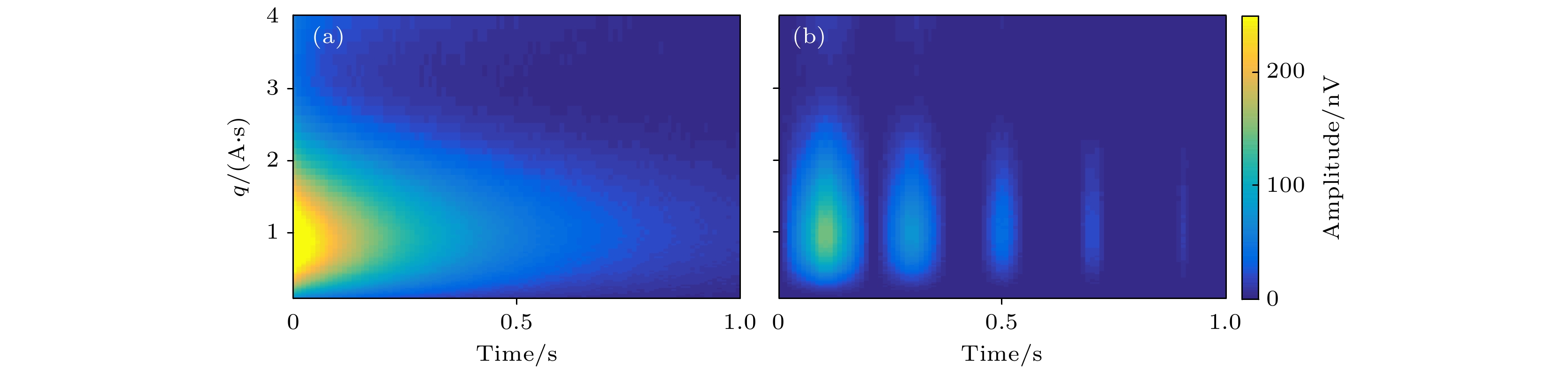 图 4 单匝100 m方形发射/接收线圈探测配置下, 同一含水情况下的地面磁共振响应(a) FID与(b) SE信号(填充颜色反映对应激发脉冲矩, 其FID或SE信号随时间衰减的磁共振信号幅度)


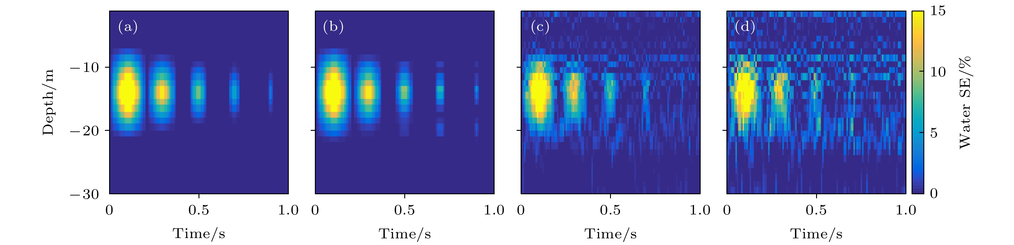 图 5 (a)模型与其在(b)无噪声, (c) 3 nV及(d) 6 nV高斯白噪声情况下的SVD线性空间反演结果


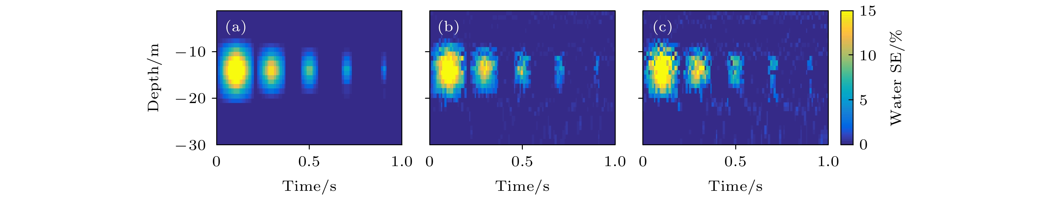 图 6 (a)模型与其在(b) 3 nV和(c) 6 nV高斯白噪声情况下的SVD与SIRT联合线性空间反演结果
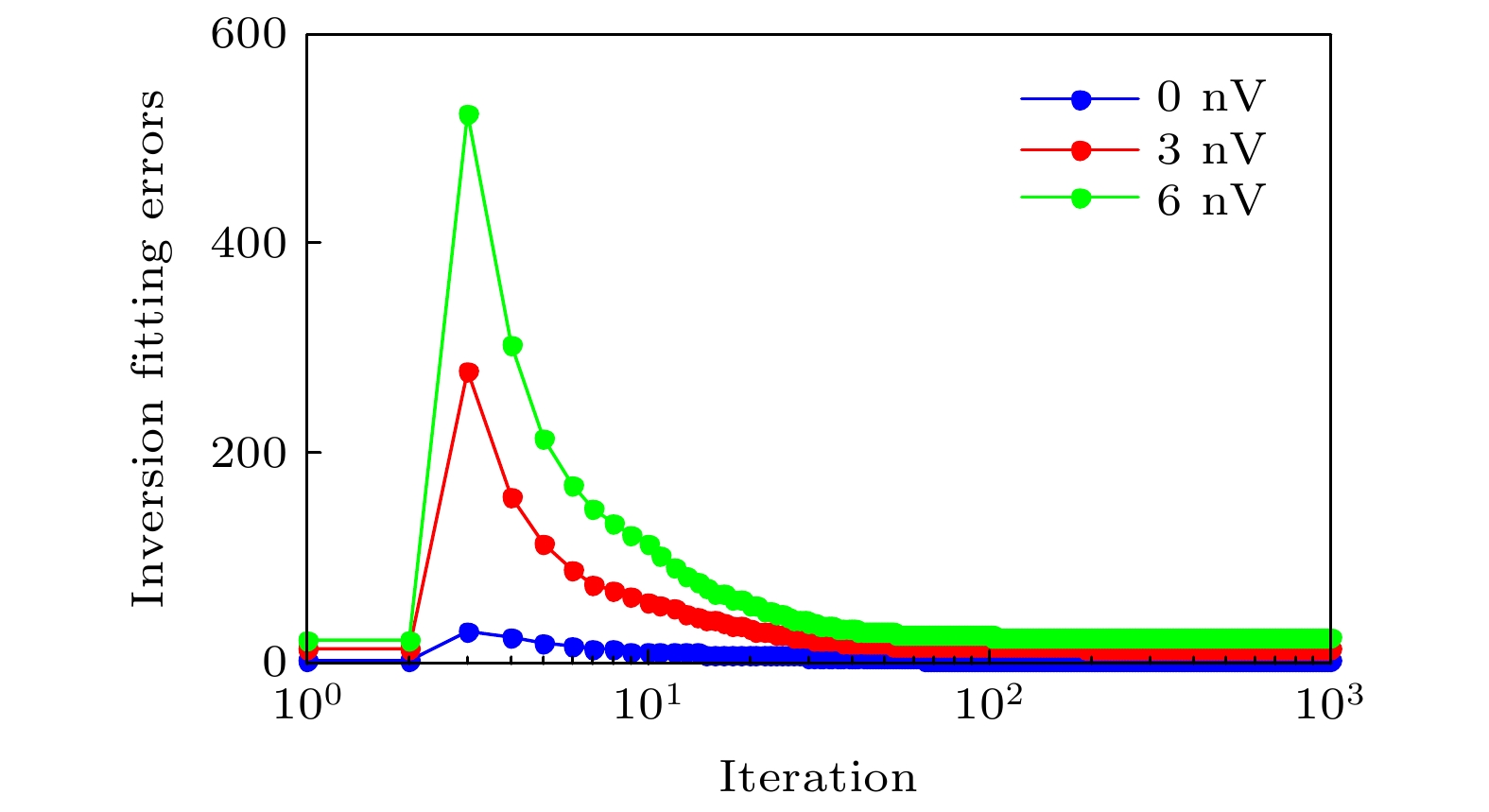 图 7 不同噪声情况下, SIRT线性空间反演迭代次数与拟合误差间的关系


 图 8 地面磁共振SE信号线性空间反演及含水量-横向弛豫时间分布拟合示意图


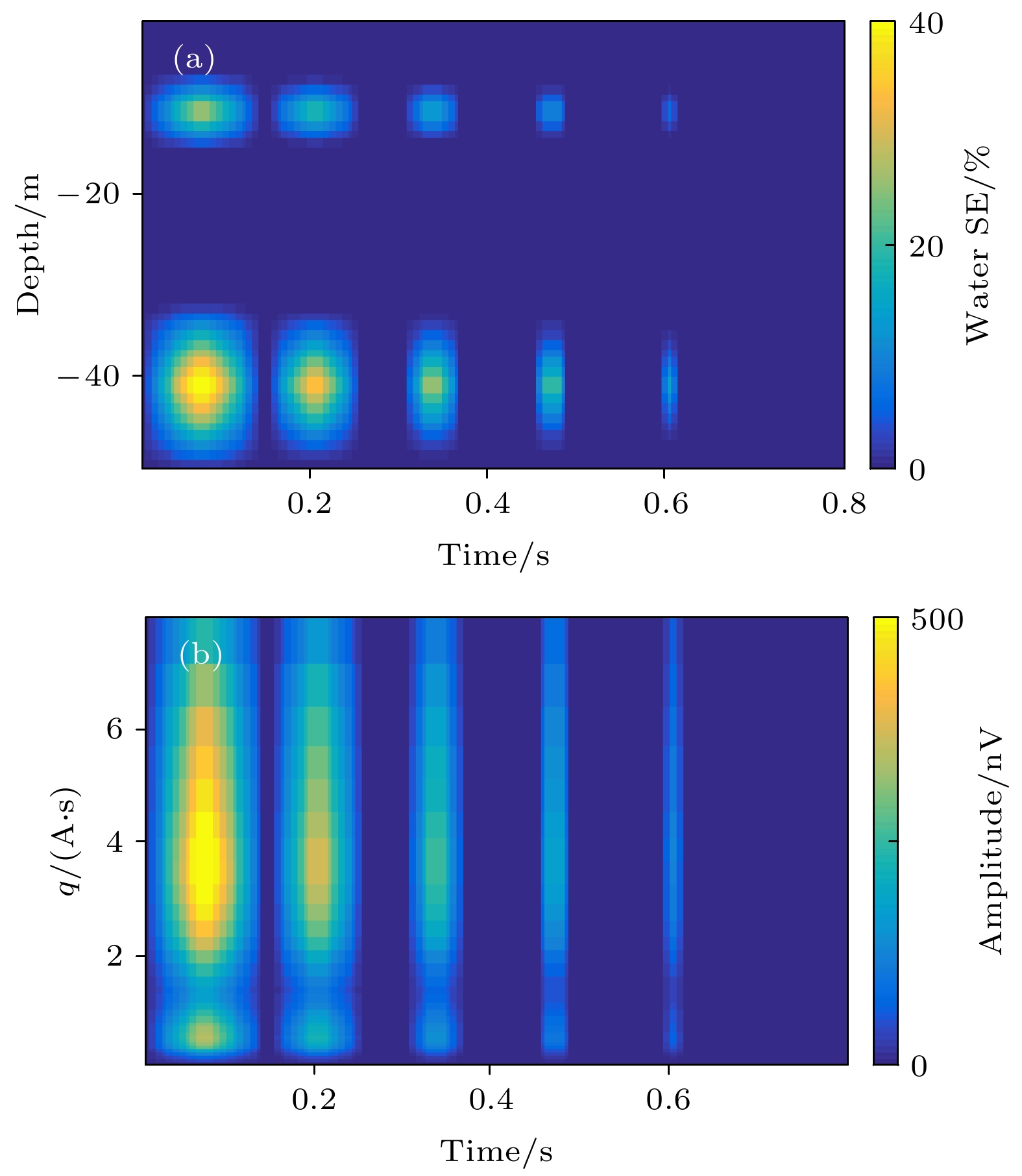 图 9 (a)地面磁共振CPMG探测实验模型与(b)正演数据(加入3 nV高斯白噪声), 假设地下存在两个含水层, 分别分布在–5 m至–15 m及–30 m至–50 m.
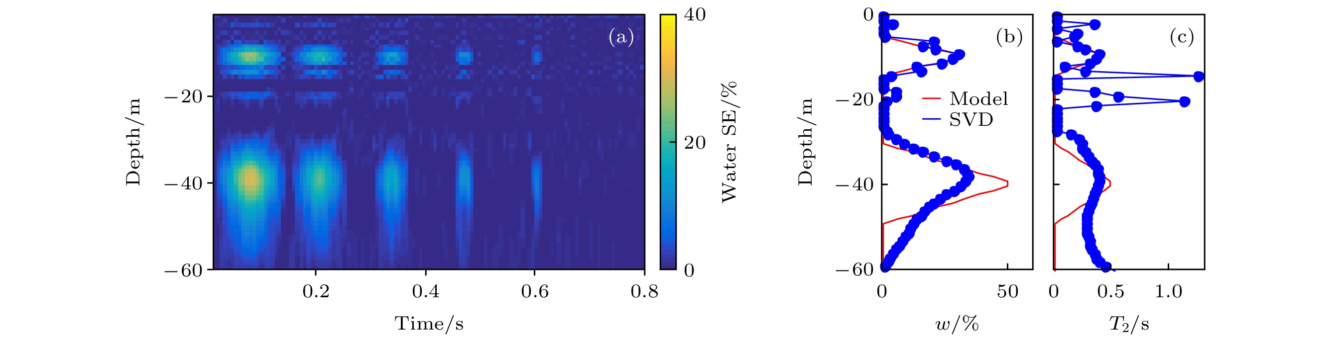 图 10 加入3 nV高斯白噪声的地面磁共振仿真数据SVD线性空间反演结果 (a) 地下水SE响应随深度及接收时间的变化; (b)与(c)分别为应用15 ms时间窗(单指数)拟合得到的w与T2分布结果


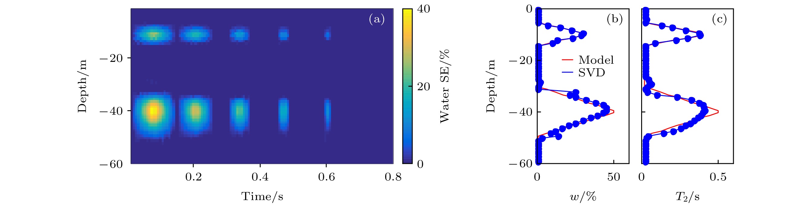 图 11 加入3 nV高斯白噪声的地面磁共振仿真数据SVD与SIRT线性空间反演结果 (a) 地下水SE响应随深度及接收时间的变化; (b)与(c)分别为应用15 ms时间窗(单指数)拟合得到的w与T2分布结果


