1.Graduate School of China Academy of Engineering Physics, Beijing 100088, China 2.School of Electrical and Electronic Engineering, North China Electric Power University, Beijing 102206, China 3.Institute of Applied Physics and Computational Mathematics, Beijing 100094, China
Fund Project:Project supported by the National Natural Science Foundation of China (Grant No. 11675021)
Received Date:17 July 2020
Accepted Date:15 September 2020
Available Online:03 January 2021
Published Online:20 January 2021
Abstract:The proton imaging system is composed of four quadrupole magnetic lenses and a collimator. The quadrupole magnetic lenses can realize point-to-point imaging, and the collimator can improve image quality by controlling proton flux and realize material diagnosis. The magnetic field gradient of an ideal quadrupole lens becomes zero at the edge. Inside the lens, the magnetic field gradient is constant along the axis, while the magnetic field boundary of the actual lens extends outward. In the proton imaging system, the fringing field will affect the proton transport state and the performance of the imaging system as well. In this paper, a method to optimize the system is presented when the fringe field is considered. A proton imaging system of 1.6 GeV is established with the Geant 4 program, in which the magnetic field gradient distribution of the actual lens is approximated by the Bell function. In an ideal imaging system, the external drift length is 1.2 m, the internal drift length is 0.5 m, the length of the magnet is 0.8 m, and the magnetic field gradient is 8.09 T/m. The parameters of the practical imaging system can be obtained by using the optimization method: when the integral difference in magnetic field gradient distribution between the actual lens and the ideal lens is equal to zero, the outer drift length of the imaging system is 1.203 m and the inner drift length is 0.506 m; when the integral difference in the magnetic field gradient distribution between the actual lens and the ideal lens is equal to 1%, the outer drift length is 1.208 m and the inner drift length is 0.516 m. In the numerical simulation, a 1mm-thick copper plate and a concentric ball are chosen as the objects, and the influence of the fringing field on the collimator aperture and that on the proton flux error are studied. The results show that the optimized imaging system can reduce the flux error of protons passing through the object, and the difference in the aperture of collimator is on the order of 10–2 when the integral difference is on the order of 10–2 in magnitude. Keywords:proton radiography/ angle-cut collimator/ fringe field of the quadrupole lens/ Geant 4 code
表2优化后质子成像系统参数 Table2.Parameters of proton imaging system after optimization.
图 5 等效漂移距离相对值的优化曲线 (a) 积分差值为0; (b) 积分差值为1% Figure5. Optimized curves of relative value of the equivalent drift distance: (a) The difference of integral value is 0; (b) the difference of integral value is 1%.
3.磁场边缘效应对准直器孔径的影响质子成像系统如图1所示. 质子运动到中心平面时, 质子的位置仅与多次库伦散射角有关, 因此可以通过角度准直器控制质子通量, 从而实现调节对比度、密度重建和材料诊断. 因此, 质子通量的准确性影响着重建密度的误差和材料诊断的准确性. 角度准直器可以通过视场半径、截断角和传输矩阵进行设计, 椭圆台状的角度准直器能保证质子通量的准确性[27]. 优化后的成像系统将改变传输矩阵, 从而影响准直器孔径形状. 图6和图7分别是影响准直器前端和后端孔径的传输矩阵元 (${m_{11}}$和${m_{12}}$)随积分差值变化的曲线, 积分差值的变化范围是(0, 7%). 图6(a)是前端口x方向的传输矩阵元变化曲线, 其中${m_{11}}$和${m_{12}}$的最大变化量分别是2%和6%; 图6(b)是前端口y方向的传输矩阵元变化曲线, 其中${m_{11}}$和${m_{12}}$的最大变化量分别是1%和4%; 图7(a)是后端x方向的传输矩阵元变化曲线, 其中${m_{11}}$和${m_{12}}$的最大变化量分别是5%和4%; 图7(b)是后端y方向的传输矩阵元变化曲线, 其中${m_{11}}$和${m_{12}}$的最大变化量是分别是2%和4%. 图 6 前端口传输矩阵元随磁场梯度积分差值的变化 (a) x方向; (b) y方向 Figure6. Transfer matrix elements of the front port varies with the gradient integral difference: (a) x direction; (b) y direction.
图 7 后端口传输矩阵元随磁场梯度积分差值的变化 (a) x方向; (b) y方向 Figure7. Transfer matrix elements of the back port varies with the gradient integral difference: (a) x direction; (b) y direction.
表3准直器孔径参数 Table3.Aperture parameters of the angle-cut collimator.
图8和图9是客体在积分差值等于0时的通量结果. 图8(a)是截断角2 mrad时铜板的通量分布, 优化前系统中的通量值与理想系统中的通量值在边缘处相差(通量差值)最大, 在$ \pm 49\;{\rm{mm}}$处二者相差3.7%, 而优化后的通量差值是0.5%. 图8(b)是截断角为3.5 mrad时的通量分布, 在$ \pm 49\;{\rm{mm}}$处, 优化前后的通量差值分别是1.3%和0.1%. 图9(a)是截断角为2 mrad时同心球客体的通量分布, 在$ - 1\;{\rm{mm}}$处, 优化前后的通量差值分别是2.0%和1.1%. 图9(b)是截断角为3.5 mrad时同心球客体的通量分布, 在$ - 1\;{\rm{mm}}$处, 优化前后的通量差值分别是0.9%和0.2%. 图 8 积分差值为0时质子通过铜板的通量分布 (a) 2.0 mrad; (b) 3.5 mrad Figure8. Flux distribution after passing the round copper plate while the integral difference is 0: (a) 2.0 mrad; (b) 3.5 mrad
图 9 积分差值等于0时质子通过同心球的通量分布 (a) 2.0 mrad; (b) 3.5 mrad Figure9. Flux distribution after passing the concentric spheres while the integral difference is 0: (a) 2.0 mrad; (b) 3.5 mrad
图10和图11是客体在积分差值等于1%时的通量结果. 图10(a)是截断角为2 mrad时铜板的通量分布, 在$ \pm 49\;{\rm{mm}}$处, 优化前后的通量差值分别是38.6%和0.1%. 图10(b)是截断角为3.5 mrad时的通量分布, 在$ \pm 49\;{\rm{mm}}$处, 优化前后的通量差值分别是23.9%和0.1%. 图11(a)是截断角2 mrad时同心球客体的通量分布, 在$ \pm 34\;{\rm{mm}}$处, 优化前后的通量差值分别是9.3%和0.5%. 图11(b)是截断角3.5 mrad时同心球客体的通量分布, 在$ \pm 34\;{\rm{mm}}$处, 优化前后的通量差值分别是8.1%和0.3%. 图 10 积分差值等于1%时质子通过铜板的通量分布 (a) 2.0 mrad; (b) 3.5 mrad Figure10. Flux distribution after passing the round copper plate while the integral difference is 1%: (a) 2.0 mrad; (b) 3.5 mrad.
图 11 积分差值等于1%时质子通过同心球的通量分布 (a) 2.0 mrad; (b) 3.5 mrad Figure11. Flux distribution after passing the concentric spheres while the integral difference is 1%: (a) 2.0 mrad; (b) 3.5 mrad.
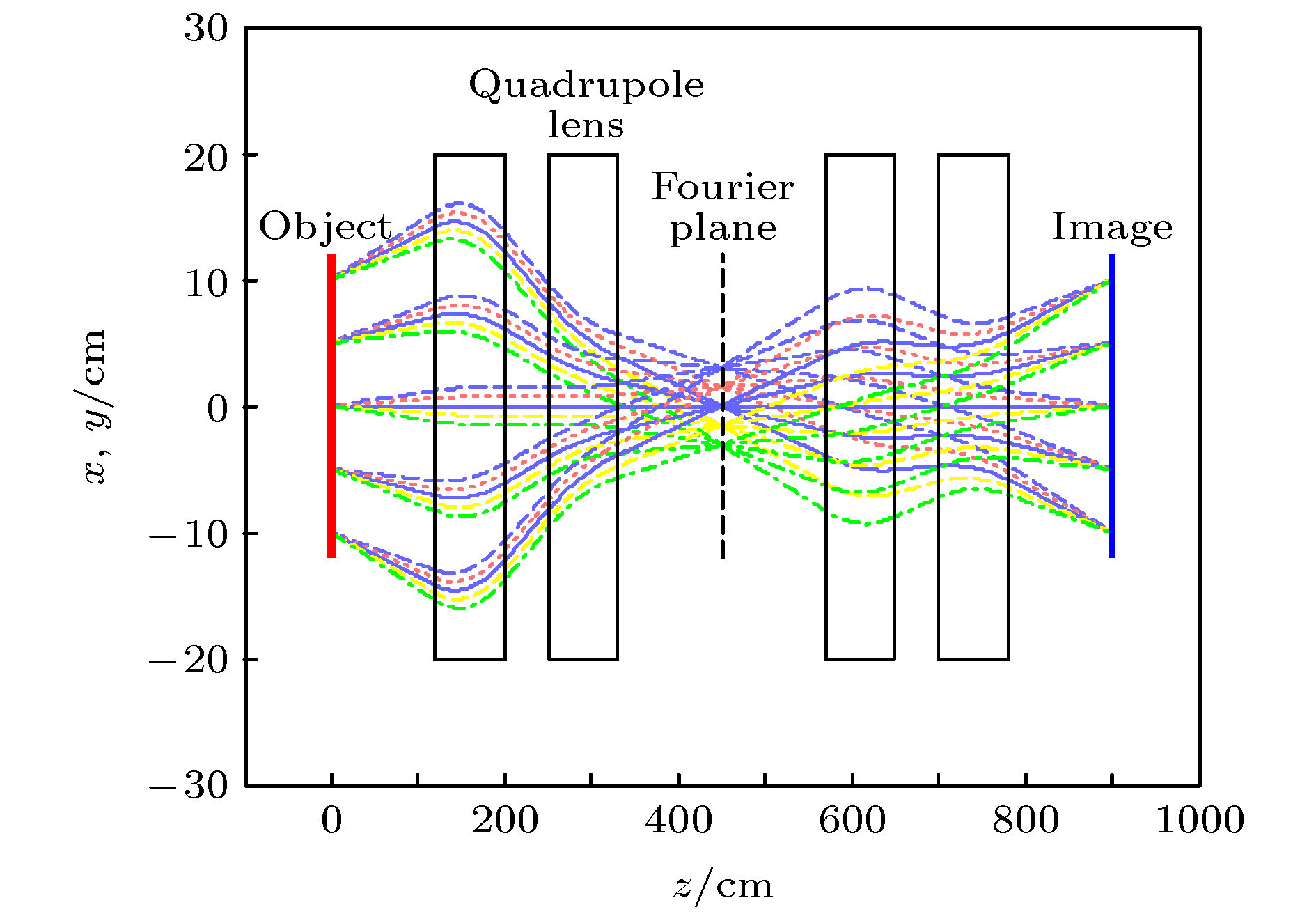 图 1 质子成像系统示意图
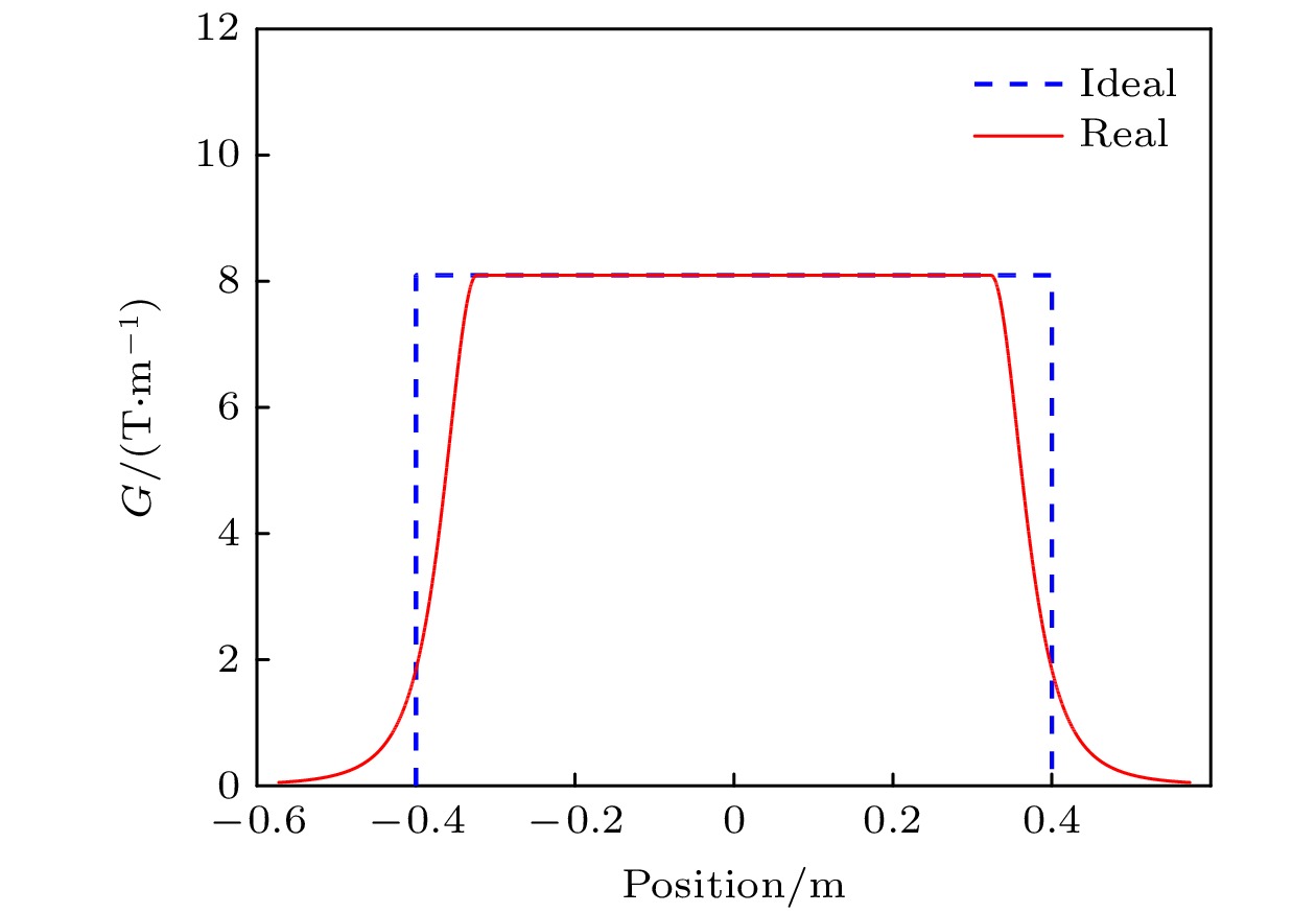 图 2 磁透镜中磁场梯度分布


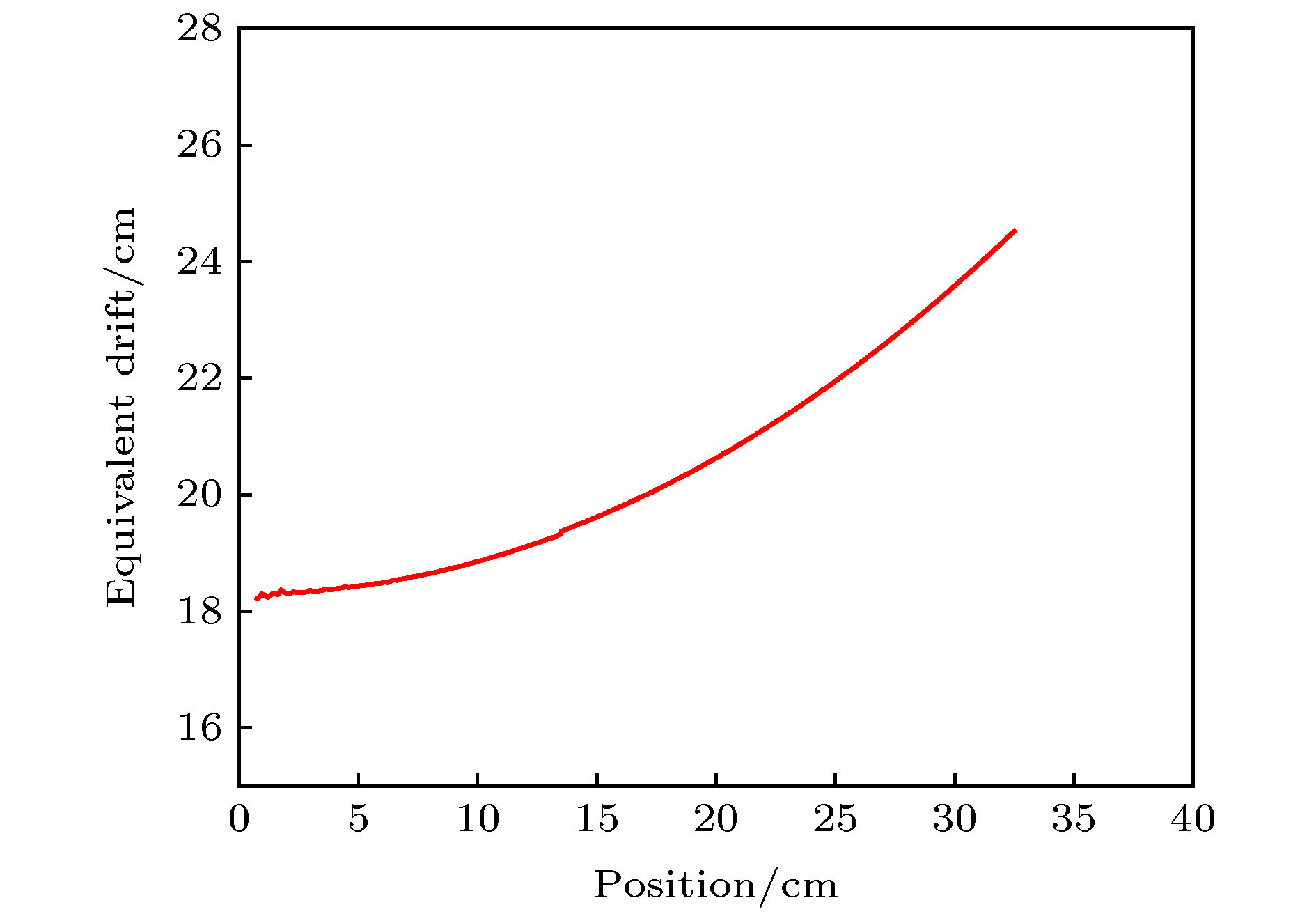 图 3 等效漂移距离随着初始位置的改变


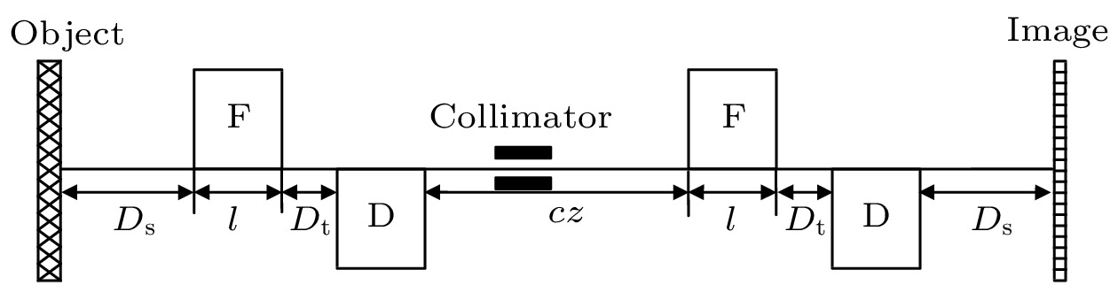 图 4 质子成像系统参数示意图
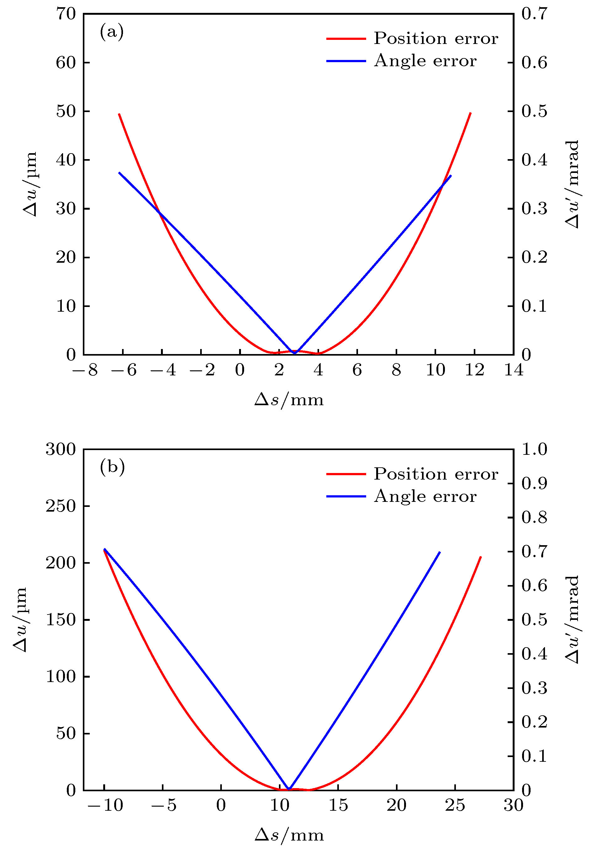 图 5 等效漂移距离相对值的优化曲线 (a) 积分差值为0; (b) 积分差值为1%


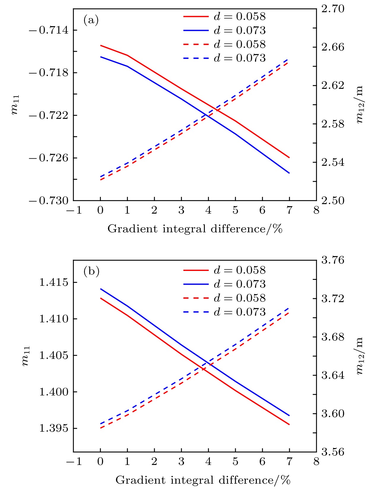 图 6 前端口传输矩阵元随磁场梯度积分差值的变化 (a) x方向; (b) y方向
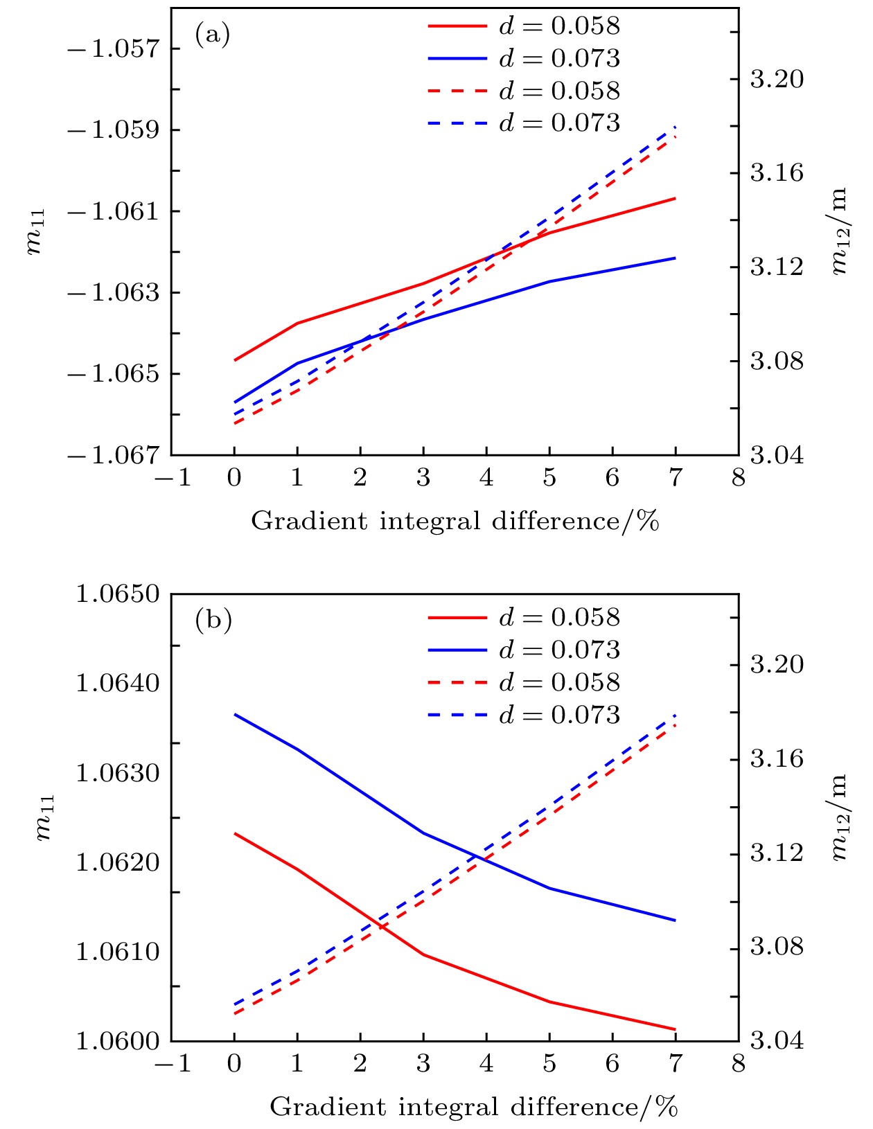 图 7 后端口传输矩阵元随磁场梯度积分差值的变化 (a) x方向; (b) y方向


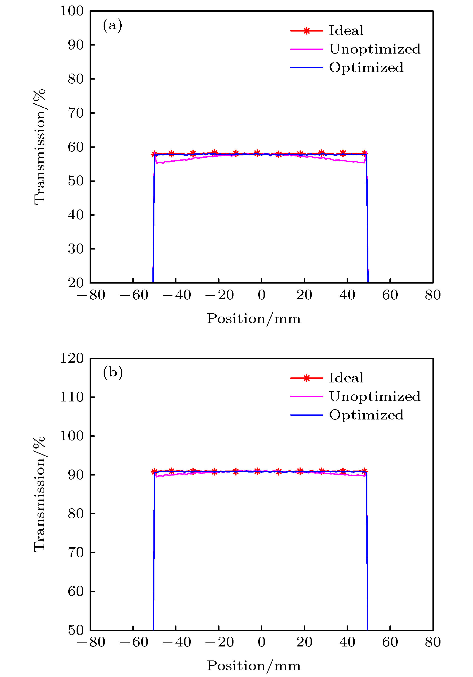 图 8 积分差值为0时质子通过铜板的通量分布 (a) 2.0 mrad; (b) 3.5 mrad
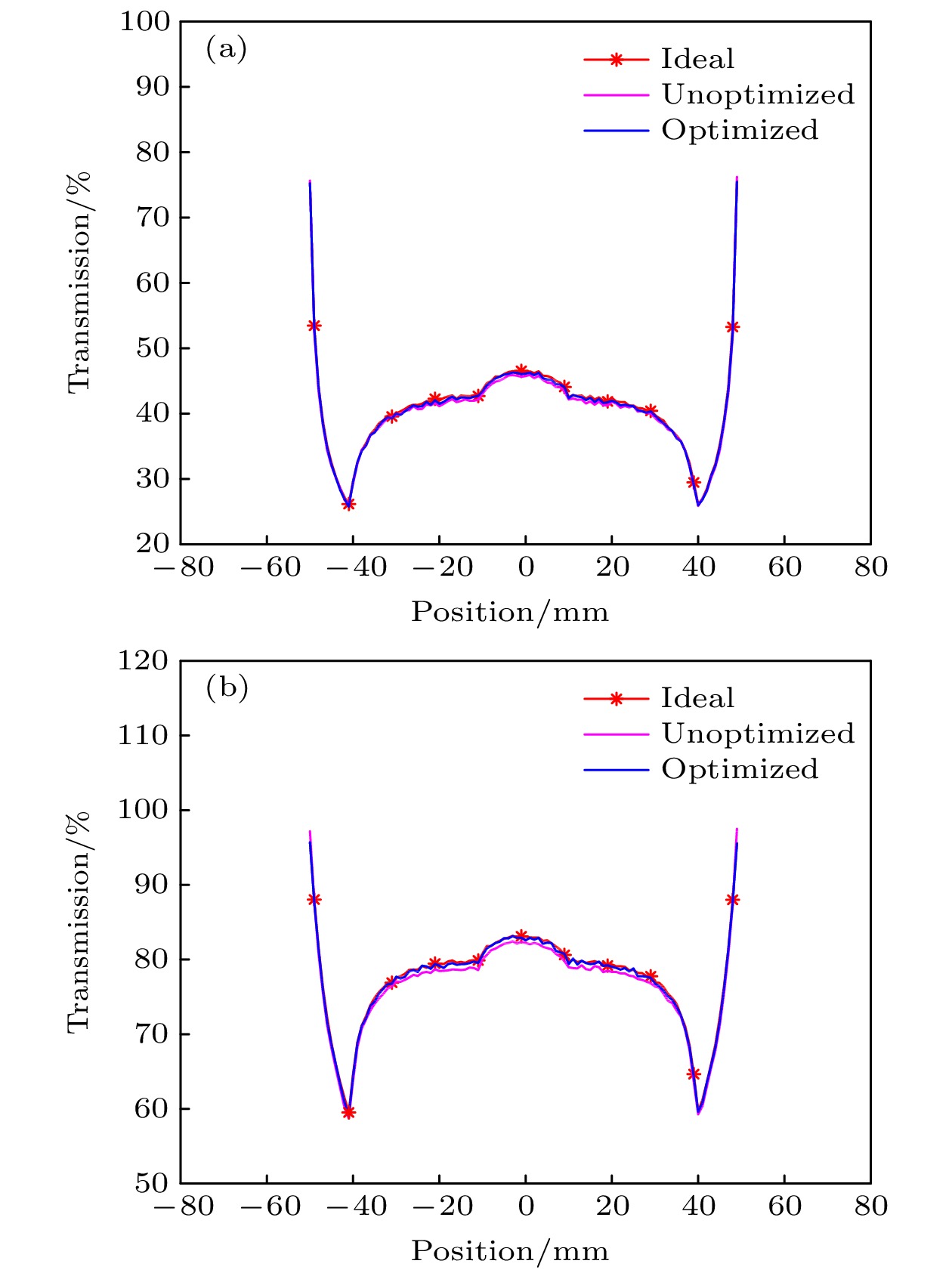 图 9 积分差值等于0时质子通过同心球的通量分布 (a) 2.0 mrad; (b) 3.5 mrad


 图 10 积分差值等于1%时质子通过铜板的通量分布 (a) 2.0 mrad; (b) 3.5 mrad
 图 11 积分差值等于1%时质子通过同心球的通量分布 (a) 2.0 mrad; (b) 3.5 mrad